Evaluating two statistical methods for handling dropout impact in repeated measures data: a comparative study on missing at random assumption

Introduction: Dropout is a major source of missing data in repeated measures studies and can bias statistical inference if not handled properly. This study compares the performance of two common methods for addressing dropout under the missing at random (MAR) assumption: multiple imputation (MI) and inverse probability weighting (IPW).

Methods: A simulation study was conducted using repeated measures data generated from a marginal regression model with continuous outcomes. Two sample sizes (100 and 250) and three dropout rates (5%, 15%, and 30%) were considered. The methods were evaluated based on bias, coverage, and mean square error (MSE). In addition, the approaches were applied to serum cholesterol data from the National Cooperative Gallstone Study to illustrate their practical performance.

Results: Simulation results showed that MI consistently produced lower bias and MSE and higher coverage compared to IPW, particularly at moderate to high dropout rates. The empirical analysis of serum cholesterol data indicated that while both methods yielded similar inferential conclusions regarding treatment effects, MI estimates were more stable and precise than those obtained from IPW.

Discussion: This analysis demonstrates that MI outperforms IPW in handling MAR dropout for continuous repeated measures data. The findings support the use of MI as a more reliable approach, especially in studies with moderate to high dropout rates, although IPW may remain acceptable under low dropout rate.

Introduction

In repeated measures studies, missing data due to dropout presents a significant challenge. These studies involve collecting data from individuals at multiple time points in a longitudinal framework. Problems arise when participants exit the study prematurely, before the designated follow-up period ends. Such dropouts can complicate statistical analysis by introducing substantial bias into the results. To better comprehend the impact of dropout in repeated measures data, it is essential to examine the underlying assumptions of incomplete measurements. According to Rubin [1], there are three missingness assumptions one can consider, namely that data are missing completely at random (MCAR), meaning that the likelihood of dropout is unrelated to either the observed data or the values that are missing; missing at random (MAR), implying that dropout is unrelated to the unobserved values, conditional on the observed data; and missing not at random (MNAR), wherein dropout depends on both missing and observed measurements.

Two methods are frequently utilized to handle incomplete longitudinal data subject to dropout under the MAR assumption. The first, known as multiple imputation (MI), involves imputing incomplete measurements and then conducting statistical analysis as if the imputed values were observed. Originally proposed by Rubin [2], MI has been extensively detailed in previous studies [2–6]. This method necessitates the MAR assumption [7]. The second method, called inverse probability weighting (IPW), adjusts for dropout by weighting the complete cases according to the inverse of their observation probabilities. This method was put forth by [8], who highlighted that IPW necessitates the dropout assumption to adhere to MAR. As mentioned in [5], IPW does not demand a comprehensive outline of the joint distribution of repeated measures outcomes since it relies on the specification of the initial two moments. More information on IPW can be found in the references [9–12].

In prior research, the comparison between MI and IPW in a cross-sectional context revealed comparable performance, with MI being marginally more efficient than IPW [12]. When assessing survey data, Seaman and White [9] evaluated the performance of MI in comparison to IPW. Their study has demonstrated why IPW might sometimes be favored, even though MI is generally more efficient. A comparative analysis of these methods through marginal structural models revealed that MI exhibited slightly less bias and significantly reduced variability compared to IPW [13]. Other studies [14–18] have compared the performance of MI and IPW and concluded that MI is generally more efficient than IPW. While both methods have been extensively compared for repeated measures data with binary outcomes, their comparison in continuous outcomes remains relatively unexplored. This study primarily concentrates on comparing MI and IPW when analyzing repeated measures data with dropouts, specifically focusing on the continuous outcomes case.

This study aims to compare the utilization of MI and IPW when faced with dropouts within repeated measures for continuous outcomes. The dropout assumption is presumed to be MAR. A comparison is carried out utilizing the estimations derived from a marginal regression model. The performance of MI and IPW is evaluated through simulated data with varying sample sizes and dropout rates and assessed using three key statistical criteria: bias, coverage, and mean squared error (MSE). The methods are also compared using data from a serum cholesterol trial.

Methodology

Notation and concepts

Consider a study where there are n individuals and each individual i is to be measured repeatedly on a set of t_i times (i = 1, . . . , n). The notation t_i allows different individuals to have unequal measurements, which includes the case where some individuals may have missing values. Let Y_ij be a t_i×1 response vector for individual i at time j, where i = 1, 2, …, n and j = 1, 2, …t_i, and let X_ij be a corresponding vector of covariates with length p. Assuming the response is continuous, the model postulates that Y_ij is a linear function of given covariates that can be expressed via a linear regression framework as follows:

$\begin{array}{ll}{Y}_{ij}={{\beta }_0+{\beta }_{1}X}_{ij1}+{\beta }_2{X}_{ij2}+\dots +{{\beta }_{p}X}_{ijp}+e_{ij},& (1)\end{array}$

where β₁, β₂, …, β_p is a p×1 vector of unknown regression parameters and e_ij are random error terms that follow a normal distribution, with mean zero and variance σ², representing discrepancies between the responses and their respective predicted means based on the model:

$\begin{array}{ll}E(Y_{ij}|X_{ij})={\beta }_0+{\beta }_1{X}_{ij1}+{\beta }_2{X}_{ij2}+\dots +{\beta }_p{X}_{ijp.}& (2)\end{array}$

For repeated measures data, e_ij are expected to be correlated within individuals, i.e, Cov(e_ij, e_ik)≠0 where j≠k. In the case of correlated data, marginal models serve as an extension of general linear models. Thus, for marginal models, the marginal mean of Y_ij is given by:

$\begin{array}{ll}E(Y_{ij}|X_{ij})={\mu }_{ij}.& (3)\end{array}$

This equation is conceptualized as a function of X_ij through a predetermined link function as given below:

$\begin{array}{ll}g({\mu }_{ij})={\eta }_{ij}=X_{ij}^{\text{'}}\beta .& (4)\end{array}$

Moreover, the variance of Y_ij is posited to be associated with its respective marginal mean, μ_ij through

$\begin{array}{ll}Var(Y_{ij}|X_{ij})=\nu ({\mu }_{ij})\phi ,& (5)\end{array}$

where ν(μ_ij)φ represents a predetermined variance function and φ embodies a scale parameter that is either known a priori or is subject to estimation. The correlation existing between Y_ij and Y_ik is mathematically determined by their respective means μ_ij and μ_ik. In general, marginal models are best suited for situations where the primary objective lies in determining population averages, while also accounting for within-individual correlations in responses. As stated in the study of Fitzmaurice et al. [10], marginal models focus on the mean response's dependence on relevant covariates, but not on random effects or prior responses. Essentially, they do not necessitate a thorough specification of longitudinal response joint distribution; instead, they require only a regression model for mean response. As a result, these models offer a versatile approach to modeling various response variables, including continuous responses.

To characterize the marginal models for a continuous response, consider Y_ij as a continuous response variable, and our goal is to determine how the changes in mean response over time rely on specific covariates. The marginal model for Y_ij is represented through the mean of Y_ij, which shows a correlation with the covariates via an identity link function, symbolized as ${\mu }_{ij}=X_{ij}^{\prime }\beta$. By using an identity link, the expected value of Y_ij is effectively a linear amalgamation of the predictor variables and their associated regression coefficients. The assumption of constant variance over time may not always be realistic; therefore, to make it more flexible, a distinct scale parameter φ_j can be estimated for the jth occasion when dealing with balanced longitudinal designs in terms of time. Accounting for the correlations between measurement occasions leads to increased efficiency in estimating regression parameters. The correlation among repeated responses within individuals is modeled by presuming an appropriate covariance structure, like a first-order autoregressive AR(1) covariance structure:

$\begin{array}{ll}Cor(Y_{ij},Y_{ik}|X_{ij},X_{ik})={\rho }^{|k-j|},0\le \rho \le 1,& (6)\end{array}$

where covariance can be described by the variances and correlations modeled by a parameter ρ, since accounting for the correlations between measurement occasions leads to increased efficiency in estimating regression parameters. It is important to note that marginal models allow for separate modeling of mean responses and within-individual dependencies. This distinction plays a crucial role in interpreting regression parameters in the mean response model, primarily in how certain covariate effects on average responses differ within sub-populations.

Missing at random (MAR)

Let R_ij be a binary indicator variable, with R_ij = 1 when Y_ij is observed and R_ij = 0 when Y_ij is missing. As a result, we divide the data vector Y_i into $Y_i=(Y_i^o,Y_i^m)$ denoting observed and missing measurements, respectively. Generally, it is essential to consider the density of the complete data f(R_i, Y_i|X_i, θ, γ), where X_i is the covariate matrix associated with individual i, containing their predictor information, while θ and γ denote parameter vectors for measurements and dropout processes correspondingly. Following the definition from [1], the dropout assumption is classified as MAR when

$\begin{array}{ll}P(R_i|Y_i,X_i,\gamma )=P(R_i|Y_i^o,X_i,\gamma ).& (7)\end{array}$

In the case of the i^th individual, the occurrence of a dropout is signified by an ordinal variable:

$\begin{array}{ll}{D}_i=1+{\displaystyle \sum _{j=1}^n}{R}_{ij}.& (8)\end{array}$

Consequently, the dropout model can be reformulated as:

$\begin{array}{ll}P(R_i|Y_i,X_i,\gamma )=P(D_i=d_i|Y_i,X_i,\gamma ),& (9)\end{array}$

where d_i represents a specific value taken by the dropout variable D_i. Each subject is measured at the first time point implying that D_i takes on values from 2 to n+1. Through this formula, the MAR model is expressed as follows:

$\begin{array}{ll}P(R_i|Y_i,X_i,\gamma )=P(D_i=d_i|Y_i^o,X_i,\gamma ),& (10)\end{array}$

meaning that dependence on Y_i occurs exclusively through its observed components $Y_i^o$. This study assumes a monotone dropout pattern, where if Y_ij is missing, then all subsequent responses Y_i(j+1), …Y_i(n) are also missing. Here, n denotes the total number of scheduled measurement occasions for individual i.

Multiple imputation (MI)

This method relies on simulation and involves replacing missing values multiple times to create several complete datasets [2]. MI essentially involves three separate tasks. First, the imputation task entails replacing missing measurements M times to create M complete datasets. During this process, the data augmentation algorithm assumes a joint distribution of fully observed measurements and prior distribution of parameters to produce random numbers of values for the missing measurements. When the MAR assumption is in place, M independent random values can be derived from the conditional distribution pertaining to unobserved measurements. Moreover, when MAR holds true, plausible values for missing observations $Y_i^m$ (m = 1, 2, 3, …, M) can be produced based on observed data $(Y_i^o,X_i,\gamma )$ and by implementing an appropriate imputation model $P(Y_i^m|Y_i^o,X_i,\gamma )$. The second task, known as the analysis task, involves analyzing these M completed datasets using standard statistical techniques, such as the marginal regression model, in order to derive required statistical inferences. Finally, during the pooling task, estimates derived from all M analyses are combined to create a single inference accounting for both sampling variability and dropout-related variability. As per the theoretical description provided by [8], missing measurements can be substituted with values derived from a MI model. Here, let $\widehat{\beta }$ represent β's complete data estimator and $\widehat{V}$ signifies its estimated variance. For the m^th imputed dataset (m = 1, 2 , 3, …, M), we can denote their values as ${\widehat{\beta }}_m$ and ${\widehat{V}}_m$. According to Rubin [19], β can be estimated using ${\widehat{\beta }}_M,$ while $var({\widehat{\beta }}_M)$ can be estimated through ${\widehat{V}}_M$ where

$\begin{array}{ll}{\widehat{\beta }}_M=\frac{1}{M}{\displaystyle \sum _{m=1}^M}{\widehat{\beta }}_m,& (11)\end{array}$

and

$\begin{array}{l}{\widehat{V}}_M=\frac{1}{M}{\displaystyle \sum _{m=1}^M}{\widehat{V}}_m+(1+M^{-1}){(M-1)}^{-1}\\ \times {\displaystyle \sum _{m=1}^M}({\widehat{\beta }}_m-{\widehat{\beta }}_M){({\widehat{\beta }}_m-{\widehat{\beta }}_M)}^T.& (12)\end{array}$

Inverse probability weighting (IPW)

As noted by Robins et al. [8], IPW is suited for handling MAR dropouts in repeated measures but necessitates the definition of a dropout model concerning observed measurements. While prevalent in marginal models featuring discrete outcomes, IPW has not been as frequently employed with continuous measurements. Nevertheless, this article focuses on employing IPW for continuous measurements, thereby mitigating biases stemming from MAR dropouts. Following the explanation put forth by Carpenter et al. [12], we first demonstrate the concept of weights in IPW. Assuming individual i's probability of being observed at time j is represented by π_ij, w_ij should be assigned as a weight to minimize any biases arising from dropout occurrences during analysis. This particular weight, ω_ij, is determined as the reciprocal of the product of cumulative probabilities for ith individual at time j.

$\begin{array}{ll}{\widehat{\omega }}_{ij}(\widehat{\alpha })={({\widehat{\pi }}_{i1}(\widehat{\alpha })\times {\widehat{\pi }}_{i2}(\widehat{\alpha })\times \dots {\widehat{\pi }}_{ij}(\widehat{\alpha }))}^{-1},& (13)\end{array}$

where $\widehat{\alpha }$ represents a q-dimensional vector comprising the parameters to be estimated. To restate, the likelihood of an individual i remaining in the study at time j should be considered as $1/{\widehat{\pi }}_{ij}$ individuals rather than one for subsequent analyses. This corresponds to one time for themselves and $\frac{1}{{\widehat{\pi }}_{ij}}-1$ times for others who drop out with the same past responses and covariates. It is important to mention that an observation with a low chance of being observed will have a higher weight. Let us designate

$\begin{array}{ll}{\lambda }_{ij}(\alpha )=P\left[R_{ij}=0|R_{i(j-1)}=1,X_i,Y_{i(j-1)},\alpha \right]& (14)\end{array}$

as the dropout probability for the ith individual at occasion j, while considering the history of all previously observed response values up to j−1. Commonly, it is presumed that all individuals are present at the initial occasion, which in turn makes λ_i1(α) = 0. The unknown quantity λ_ij(α) must be assessed from existing data by employing a logistic model: $logit({\lambda }_{ij}\left(\alpha \right))={\alpha }^{\prime }{Z}_{ij}$, where Z_ij is a vector of covariates, possibly including previously observed responses and other variables believed to predict the probability of dropout. To illustrate the application of IPW for continuous responses in repeated measures, we initiate our discussion with a basic understanding of the generalized estimating equations (GEE) method as proposed by [20]. The core concept involves extending the standard univariate likelihood equations through the inclusion of a covariance matrix for the response vector, Y_i. GEE has gained significant popularity, particularly in analyzing categorical and count outcomes, while also being applicable to continuous variables. Within the context of linear statistical models, inclusive of marginal models that employ an identity link function, one can consider a generalized least squares (GLS) method as a particular case of generalized estimating equations (GEE) [10]. As a result, parameter estimates within marginal models for continuous responses accompanied by identity links are as follows:

$\begin{array}{ll}\widehat{\beta }={\left[{\displaystyle \sum _{i=1}^n}{X}_i^{\prime }{\hat{\Sigma }}_i^{-1}{X}_i\right]}^{-1}\left[{\displaystyle \sum _{i=1}^n}{X}_i^{\prime }{\hat{\Sigma }}_i^{-1}{Y}_i\right],& (15)\end{array}$

where ${\hat{\Sigma }}_i$ is the restricted maximum likelihood estimate of $\sum _i$ and

$\begin{array}{l}Cov(\widehat{\beta })={\left[{\displaystyle \sum _{i=1}^n}{X}_i^{\prime }{\hat{\Sigma }}_i^{-1}{X}_i\right]}^{-1}{\displaystyle \sum _{i=1}^n}{X}_i^{\prime }{\hat{\Sigma }}_i^{-1}{\widehat{\vee }}_i{\hat{\Sigma }}_i^{-1}\\ X_i{\left[{\displaystyle \sum _{i=1}^n}{X}_i^{\prime }{\hat{\Sigma }}_i^{-1}{X}_i\right]}^{-1},& (16)\end{array}$

where the expression ${\widehat{\vee }}_i=(Y_i-{X_i}^{\prime }\beta )(Y_i-{X_i}^{\prime }\beta )$ serves as an estimate of Var(Y_i) to achieve a robust estimator for $Cov(\widehat{\beta })$. Obtaining consistent estimates for parameters β in the weighted method requires two additional assumptions besides the MAR assumption: (1) For each time point j, the probability that subject i continues participation in the study must be positive, or more precisely:

$\begin{array}{ll}P\left[R_{ij}=1|R_{i(j-1)}=1,X_i,Y_{ij}\right]>\delta >0.& (17)\end{array}$

(2) The dropout model's probability needs to be correctly specified; hence, λ_ij(α) = P[R_ij = 0|R_i(j−1) = 1, X_i, Y_i(j−1)]. Given the MAR assumption, the probabilities of staying within the study, π_ij(α) can be calculated as follows

$\begin{array}{ll}{\pi }_{ij}(\alpha )=P\left[R_{ij}=1|R_{i(j-1)}=1,X_i,Y_{i1},\dots ,Y_{i(j-1)},\alpha \right].& (18)\end{array}$

Following the aforementioned assumptions, valid parameter estimates will be given in repeated measures data with MAR dropouts by employing the weighted estimating equations

$\begin{array}{ll}{\displaystyle \sum _{i=1}^n}{(Y_i-X_i\beta )}^{\prime }{\hat{\Sigma }}_i^{-1}{W}_i(\widehat{\alpha })=0,& (19)\end{array}$

where $W_i(\widehat{\alpha })=diag\left\{W_{i1}(\widehat{\alpha }),\dots ,W_{i{t}_i}(\widehat{\alpha })\right\}$ for j = 2, …, t_i and W_i1 = 1.

Within the framework of a weighted marginal model, designed for continuous outcomes that employ an identity link function, it is postulated that the parameter estimations in question will manifest in distinct and predictable configurations.

$\begin{array}{ll}\widehat{\beta }={\left({\displaystyle \sum _{i=1}^n}{X}_i^{\prime }{{\hat{\Sigma }}_i^{-1}{W}_i\left(\widehat{\alpha }\right)X}_i\right)}^{-1}{\displaystyle \sum _{i=1}^n}\left(X_i^{\prime }{{\hat{\Sigma }}_i^{-1}{W}_i\left(\widehat{\alpha }\right)Y}_i\right),& (20)\end{array}$

and

$\begin{array}{l}Cov\left(\widehat{\beta }\right)={\left({\displaystyle \sum _{i=1}^n}{X}_i^{\prime }{{\hat{\Sigma }}_i^{-1}{W}_i\left(\widehat{\alpha }\right)X}_i\right)}^{-1}\\ \left({\displaystyle \sum _{i=1}^n}{X}_i^{\prime }{\hat{\Sigma }}_i^{-1}{W}_i\left(\widehat{\alpha }\right)W_i{\left(\widehat{\alpha }\right)}^{\prime }{X}_i\right)\\ {\left({\displaystyle \sum _{i=1}^n}{X}_i^{\prime }{{\hat{\Sigma }}_i^{-1}{W}_i\left(\widehat{\alpha }\right)X}_i\right)}^{-1}.& (21)\end{array}$

Simulation scenario

Study design

This research investigates how MI and IPW perform in managing MAR dropout in longitudinal data settings with continuous response variables. To achieve this aim, the following procedures are implemented: (1) Complete repeated measures data with continuous outcomes were generated using 100 random samples for two sample sizes, N = 100 and N = 250. A marginal regression model was utilized to obtain parameter estimates; (2) MAR dropout scenarios were created at varying dropout rates for both sample sizes; (3) MI and IPW were applied to each simulated dataset. The results obtained from these methods were compared with those derived from complete data; and (4) to test how MI and IPW performed, the study examined bias, coverage, and mean squared error (MSE) as evaluation criteria.

Data generation

Simulated data were generated to mimic data frequently observed in longitudinal clinical trial studies. The repeated measures data with dropout were simulated by first generating complete datasets. Next, random samples of 100 were drawn in sizes N = 100 and 250 individuals. During the simulation, individuals were assumed to receive two treatment arms. Namely, the treatment variable is a binary dummy variable coded as 1 for treatment and 0 for control. Measurements were recorded at four separate time points (j = 1, 2, 3, 4). These time points are equidistant (e.g., time points at baseline, week 1, week 2, and week 4). Several studies support the selection of four time points; for instance, see [5]. The outcome of interest (Y_ij) represents the measurement of an individual i at time j. Therefore, repeated-measure data were created based on the following marginal regression model:

$\begin{array}{ll}E(Y_{ij}|T_j,Tr{t}_i)={\beta }_0+{\beta }_1{T}_j+{\beta }_{2}Tr{t}_i+{\beta }_3{T}_j^{\ast }Tr{t}_i.& (22)\end{array}$

For this model, we fixed β₀ = −0.25, β₁ = 0.5, β₂ = 1, and β₃ = 0.2. An autoregressive covariance structure of order 1 or AR(1) with ρ = 0.7 and σ = 6.0 is assumed for Y_ij. The linear regression model presented in Equation 22 explains the mean response changes over time and their relationship to the covariates, which include treatment, Trt, time, T and time-by-treatment interaction, T*Trt. Essentially, this model describes the relationship between responses at each occasion and their corresponding covariates. For each simulated dataset, dropouts in Y_ij were stochastically generated. All individuals were observed at the initial time point, with potential dropouts occurring at the second and third time points. That is, the dropout probability is modeled as P(D_i = d_i|Y_i1), where d_i denotes a specific value taken by the dropout indicator D_i. MAR dropouts were generated using a logistic regression model as given below:

$\begin{array}{ll}logit\left(R_{ij}=1|\gamma \right)={\gamma }_0+{\gamma }_1{Y}_{ij-1}+{\gamma }_2{Y}_{ij-2},& (23)\end{array}$

where the parameters γ₀, γ₁, and γ₂ are set to be −2, 1, and 0.5, respectively. Dropout rates were chosen to roughly correspond to 5%, 15%, and 30%. A monotonic dropout pattern was employed, in which data for an individual were available up until a specific time point. This simulates a scenario in which an individual's withdrawal serves as the sole cause of dropout.

Data analysis

In the imputation process, SAS PROC MI was used to fill in the dropouts for each simulated sample. The imputation model incorporated all variables found in Model (22) and employed Markov chain Monte Carlo (MCMC) sampling method to generate multiple sets of plausible values for the missing values. With a dropout rate below 30%, the chosen value for M was 5, as suggested and substantiated by [4, 21, 22], who asserted that, for a low percentage of missing data, an M value between 3 and 10 typically yields satisfactory imputation results. The imputation process began with 100 preliminary iterations and used the default settings of the SAS framework, including a Jeffreys non-informative prior and initial estimates based on the posterior mode from the EM algorithm. Finally, using SAS PROC MIXED, Model (22) was applied to each imputed dataset to obtain parameter estimations, and the results from all five datasets were combined using SAS PROC MIANALYZE to form a single inference. Conversely, IPW was employed for each of the simulated samples using SAS macros developed by [6]. IPW was employed through a three-step process: (1) creating a dropout model with an outcome variable (Y_ij) and predictors, including prior outcomes (Y_{i, j−1}) at previous occasions and relevant covariate data, using the DROPOUT macro; (2) constructing a weighted regression with inverse dropout probability weights via the DROPWGT macro, considering past non-dropout probabilities. The final factor involves the probability of either dropping out or persisting in the study; and (3) applying model (22) with an identity link function, presented in Equation 15. Alongside this marginal model, the AR(1) covariance structure is employed to represent the correlation of Y_ij within individuals, as repeated measures data typically exhibit unequal correlations between measurements on the same individual over time, but decrease as measurements get farther apart from each other. In line with established approaches for analyzing longitudinal data, the marginal regression model has been applied to estimate population-average effects in repeated measures with continuous outcomes [10]. An AR(1) covariance structure was chosen to reflect realistic within-subject correlations over time [5]. These choices contribute to a rigorous simulation framework for comparing the performance of MI and IPW under the MAR assumption.

Criteria of performance assessment

We evaluate the performance of MI and IPW primarily based on the suggested criteria in [7, 23], focusing on bias, coverage, and mean square error (MSE). First, bias is determined as: $Bias=\left(\overline{\widehat{\beta }}-\beta \right),$ where β is the actual value of the estimate being analyzed, and $\overline{\widehat{\beta }}=\sum _{i=1}^s\frac{{\widehat{\beta }}_i}{S}$, with s being the total number of simulations conducted and ${\widehat{\beta }}_i$ signifying the estimate of interest within each i = 1, 2, 3, …s simulations. Second, coverage refers to the proportion of 95% confidence interval estimates that contain the true parameter over 1,000 repetitions. As per [23], a coverage below 90% signifies a severe under-coverage as it is equivalent to double the nominal error rate (0.05). A well-functioning method should exhibit an actual coverage near the nominal rate (95%). Finally, MSE assesses parameter estimation accuracy by incorporating measures of bias and variability. It is expressed as: $MSE={\left(\overline{\widehat{\beta }}-\beta \right)}^2+{\left(SE\left(\widehat{\beta }\right)\right)}^2$, where $SE\left(\widehat{\beta }\right)$ represents the calculated standard error of the estimated value obtained from all simulations conducted in this study.

Results

Simulation results for sample size N=100

Table 1 displays the simulation results for 5%, 15%, and 30% dropout rates with regard to bias, coverage, and MSE values when N = 100 sample size.

Table 1

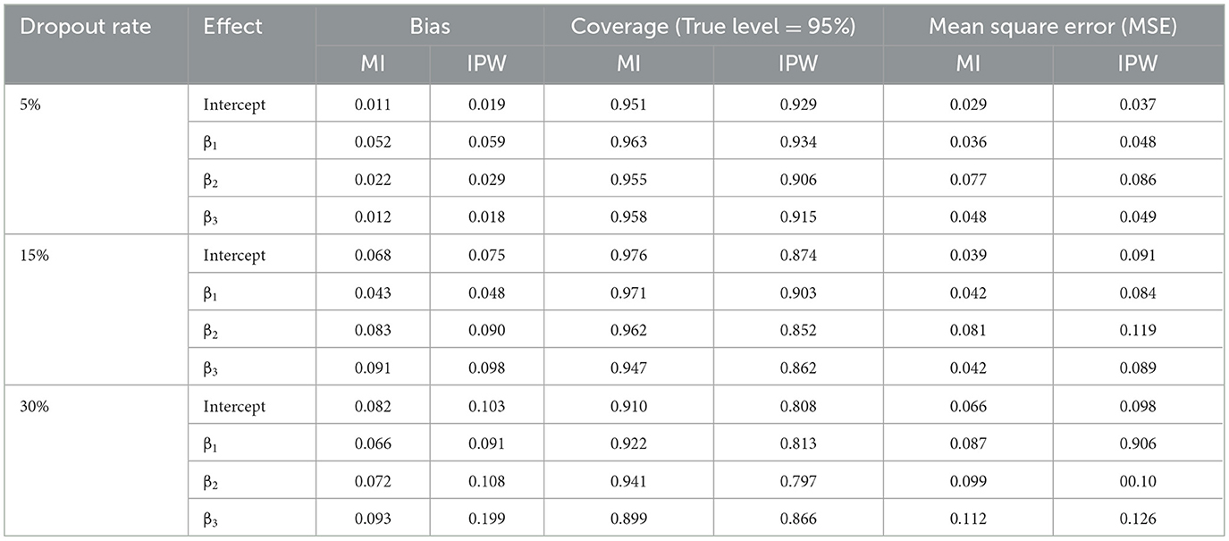
Table 1. Bias, coverage and mean square error (MSE) of MI and IPW when N = 100.

For a 5% dropout rate, it was found that the bias was lower in the MI estimates compared to IPW; however, the estimates from both methods were quite similar overall. The table also indicates that MI and IPW generated comparable coverage rates. Following the above definition of coverage, both methods offered equally relevant confidence intervals for all variables incorporated in the analysis model, with coverage rates mostly exceeding 90%. According to the rationale provided by [11], their performance does not contribute to an increased Type-I error rate. Examining the MSE criterion revealed that MI outperformed IPW in general due to its smaller estimated values. Nevertheless, the differences in MSE estimates between the two methods were minor since their values were fairly close.

A comparison of a 15% dropout rate revealed that MI consistently generated less biased estimates. Its efficient performance regarding bias was evident through all parameter estimates. Unlike the 5% dropout rate scenario, MI and IPW showed no significant similarity in coverage results. Their estimates were varied significantly in magnitude. Namely, the MI method proved to be nearly more effective at this level of dropout rate. The IPW-related MSEs were larger than those provided by MI for all cases, where IPW's MSE deteriorated. As a result, IPW's MSEs were generally worse than those generated by MI.

Regarding a 30% dropout rate, IPW-based results exhibited higher estimation bias compared to MI, signifying a discrepancy between the average estimates and true values. In terms of coverage criteria, the MI method once again demonstrated acceptable performance since its values exceeded 90%. For the MSE criterion, IPW's calculated results yielded the largest values, demonstrating no considerable improvement across varying dropout rates in comparison to MI-derived results in the considered sample size. There was no deviation from this rule for all estimates.

Simulation results for sample size N=250

Table 2 illustrates the simulation results for bias, coverage, and MSE using MI and IPW with a sample size of 250, under 5%, 15%, and 30% dropout rates.

Table 2

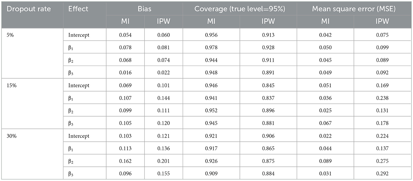
Table 2. Bias, coverage and mean square error (MSE) of MI and IPW when N = 250.

In the scenario with a 5% dropout rate, the MI method exhibits satisfactory performance, implying that its bias estimations closely align with the actual data. Nonetheless, IPW tends to generate the most biased estimates more frequently than MI, giving MI a slight edge in mitigating bias. Furthermore, coverage rates exceeding 90% were obtained by both methods, except for β₃ associated with IPW. As for MSE, IPW introduced marginally higher values, indicating no improvement in the method's performance, with an increase in sample size to 250. Overall, both methods provided completely different MSE values from each other in all cases.

Under 15% dropout rate, IPW's estimates showed greater bias compared to MI's. Additionally, MI maintained equally acceptable coverage rates with none falling below 90%. On the contrary, IPW performed poorly at the true level of 95%, as its coverage rates for all estimates dipped under 90%. In reference to MSE criteria, MI outshone IPW across all cases as the method generally displayed larger values for all parameter estimates evaluated in the analysis. This result implies that MI's performance improves as the sample size and dropout rate increase.

Finally, when examining a 30% dropout rate scenario and comparing the two methods' performance with respect to bias criteria, it is evident that MI surpasses IPW even in higher dropout situations. The increasing dropout rate also seemed to have minimal impact on the MI method's coverage performance, as MI provided estimates that exceeded 90%. This was not the case for the IPW method, which provided coverage rates less than 90% in all cases. Upon evaluating the MSE criteria, stability was observed in the performance of both methods, as the MI method provided much lower values than the IPW method. Thus, the IPW method continued to exhibit poor performance.

Figure 1 displays MSE for the MI and IPW methods across dropout rates of 5%, 15%, and 30% for sample sizes of 100 and 250. Across all parameter estimates, the MI method consistently produced lower MSE values than IPW at each dropout level and sample size, indicating higher precision. These findings underscore the superior performance of MI in addressing dropout, particularly under moderate to high dropout scenarios.

Figure 1

Figure 1. Mean squared error (MSE) for MI and IPW methods across dropout rates at sample sizes of 100 and 250.

Serum cholesterol study

Since the purpose of this study is to rigorously evaluate the performance of the MI and IPW methods by applying them to simulated data inspired by clinical trials, we also tested their performance in the case of practical application to real-world data, an important aspect of statistical validation in clinical research. In the following paragraphs, we will present an applied study to determine the performance of these two methods if they are used in real experimental data.

In this study, we present the application of the methods to data from the National Cooperative Gallstone Study (NCGS). Additional background details on this data can be found in [24]. The data involved randomly assigning 103 patients to either a high-dose (750 mg/day), a low-dose (375 mg/day), or a placebo group. The treatment period lasted for 4 weeks. Our current analysis focuses on a subset of data concerning patients with floating gallstones, who were randomly allocated to the high-dose and placebo cohorts. The NCGS proposed that chenodiol could dissolve gallstones while potentially increasing serum cholesterol levels. The NCGS aimed to determine the efficacy of chenodiol in dissolving gallstones while examining its potential impact on serum cholesterol levels. Consequently, serum cholesterol (mg/dL) measurements were taken at baseline and during 6, 12, 20, and 24 weeks of follow-up. Dropouts were prevalent in these measurements due to missed visits, loss or inadequacy of laboratory specimens, or termination of patient follow-ups. Additionally, all subjects had observed values at week 6. A segment of the patients received the study treatment (drug and placebo) but dropped out before the scheduled post-baseline period, specifically at the 12-week time point. However, other individuals dropped out either at week 20 or 24. This resulted in data reflecting three distinct dropout patterns (dropout at time points 12, 20, or 24). All 103 patients were observed during the first week, while 67, 78, and 93 patients attended during weeks 4, 3, and 2, respectively. Table 3 shows the percentage of patients continuing through each week by treatment arm. Based on a previous study of this data using sensitivity analysis, the dropout assumption has been shown to be MAR [25]. In this study, we present a detailed description at the potential influence of dropout on serum cholesterol levels. The analysis will predominantly focus on estimated parameters, standard errors, and p-values.

Table 3

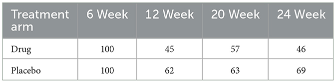
Table 3. Percentage of patients continuing in the study through each week by treatment arm.

We proceeded to apply the two statistical methodologies, MI and IPW, to a dataset comprising serum cholesterol measurements. These measurements, denoted as Y_ij, represent the serum cholesterol level recorded on the jth occasion for the ith patient. Our primary focus was to assess the impact of two different therapeutic approaches on serum cholesterol levels over time. To conduct the statistical analysis, we utilized Model (22) for both MI and IPW. For the latter, the GLS technique was employed. The results of these methods are presented in Table 4. Upon reviewing the results, it was apparent that neither method found significant treatment effects or time-by-treatment interactions; all associated p-values exceeded the 0.05 level for significance. Although both MI and IPW indicated that these effects were not statistically significant, the estimates they provided differed substantially. Furthermore, the p-values associated with the intercept and time effects diverged markedly between the two methods. MI yielded highly significant p-values, while the IPW method did not. This inconsistency also extended to the parameter estimates and standard errors, which varied greatly in magnitude between MI and IPW. In summary, our analysis revealed notable differences in the performance of the MI and IPW methods when applied to repeated measurements of continuous outcomes, such as serum cholesterol levels.

Table 4

Table 4. Parameter estimates, standard errors, and p-values received from Serum cholesterol data.

Discussion and conclusion

This study investigated the application of the MI and IPW methods for addressing incomplete repeated measures data due to an MAR dropout. The focus was limited to repeated measures involving continuous outcomes. Both methods were selected for this study as they are well-established methods to tackle problems stemming from the MAR dropout assumption. There are limited studies that compare MI and IPW for handling dropout in repeated measures with continuous outcomes, prompting this study to assess these methods' performance under varying sample sizes and dropout rates. An MAR dropout assumption was assumed under different rates. The methods were examined by employing simulated repeated measurements data with varying sample sizes. The evaluation was conducted utilizing bias, coverage, and MSE criteria for comparison. The subsequent conclusions were drawn from the results of this analytical comparison.

Throughout the range of simulations encompassing both small and large sample sizes, the MI method demonstrated superior performance, suggesting that its efficacy is not influenced by variations in sample size. The findings of the current analysis revealed that the bias associated with MI-based estimators was found to be minimal, thus confirming that the imputed values did not substantially skew the results. Consistent with the observations by eminent researchers [5, 6, 13, 19], the MI approach produces more reliable estimation provided that the imputation model is accurately specified. The results in general favored MI over IPW. This MI advantage is well documented in the previous research conducted by [26], who noted that when both IPW and MI methods are valid and correctly implemented, MI is typically more efficient. On the other hand, it was revealed that IPW demonstrated lower efficiency in comparison to MI, irrespective of the dropout rate. The results indicated a decline in performance as the dropout rate increased. This is consistent with the guidance posited in [27], which advises against employing the IPW method in instances where the MI approach is applicable, as the former is typically less efficacious due to its exclusive reweighting of complete cases and inability to incorporate incomplete auxiliary variables. Nevertheless, in scenarios characterized by a small sample size, IPW demonstrated generally acceptable performance, notably under conditions of low dropout rates. This conforms with previous findings indicating the suitability of this method when the prevalence of dropout is low [28].

Despite the observed inconsistency between MI and IPW results, it is essential to keep in mind several key aspects when examining IPW analysis for continuous outcomes in incomplete repeated measures. The reality is that the IPW approach might be more suitable for various discrete outcome categories, rather than continuous ones, when the aim is to draw conclusions about population averages instead of individual cases. Furthermore, the MI method mitigates several significant limitations inherent to direct modeling methods, such as the disproportionate influence of individual weights in IPW estimation, as discussed in [29]. The poor performance of IPW can be further justified by the fact that the primary challenge encountered in IPW performance when dealing with continuous responses in repeated measures is the computation of correlations between various measurements pertaining to the same individual. In this study, only the AR (1) covariance structure has been applied, as others created computational issues. However, this achievement is rather gratifying when compared with the analysis documented in the study by [30], where within-individual correlations were entirely ignored while employing an IPW method. Ignoring these correlations in our case may yield inefficient parameter estimates. Another drawback associated with the IPW method was that the assumed AR (1) covariance structure could be the assumption of the time-invariant scale parameter φ, which contradicts the nature of repeated measures data properties like those seen in our data, where variances between measurements generally fluctuate across different time points. As a final remark, it is crucial to acknowledge that the IPW method might be a less favorable option for handling incomplete repeated measures data when compared to more sophisticated methods, like the MI method, for continuous responses. Evidently, this finding should not be perceived as a conclusive validation but rather contributes to the existing understanding of these methods' comparative effectiveness.

Limitations and future research

While this study offers valuable insights into the comparative performance of MI and IPW under monotone MAR dropout in repeated measures data with continuous outcomes, several limitations should be acknowledged. First, the simulation design was restricted to two sample sizes and a specific marginal model with a fixed autoregressive covariance structure AR (1). In real-world scenarios, variance heterogeneity and alternative correlation structures may influence the effectiveness of dropout-handling methods. Second, the study focused exclusively on monotone dropout, whereas non-monotone patterns are common in practice and may affect method performance differently. Future research could expand the simulation framework to include non-monotone missingness, unequal measurement intervals, and more complex outcome structures. Additionally, applying the compared methods to real-world longitudinal datasets with varying dropout mechanisms would help validate the generalizability of the findings.

Data availability statement

Publicly available datasets were analyzed in this study. This data can be found here: [https://content.sph.harvard.edu/fitzmaur/ala2e/cholesterol.txt].

Author contributions

MS: Formal analysis, Writing – original draft, Methodology, Conceptualization, Software. AS: Supervision, Writing – review & editing. HM: Writing – review & editing, Supervision.

Funding

The author(s) declare that no financial support was received for the research and/or publication of this article.

Conflict of interest

The authors declare that the research was conducted in the absence of any commercial or financial relationships that could be construed as a potential conflict of interest.

Generative AI statement

The author(s) declare that no Gen AI was used in the creation of this manuscript.

Any alternative text (alt text) provided alongside figures in this article has been generated by Frontiers with the support of artificial intelligence and reasonable efforts have been made to ensure accuracy, including review by the authors wherever possible. If you identify any issues, please contact us.

Publisher's note

All claims expressed in this article are solely those of the authors and do not necessarily represent those of their affiliated organizations, or those of the publisher, the editors and the reviewers. Any product that may be evaluated in this article, or claim that may be made by its manufacturer, is not guaranteed or endorsed by the publisher.

References

1. Rubin DB. Inference and missing data. Biometrika. (1976) 63:581–92. doi: 10.1093/biomet/63.3.581

Crossref Full Text | Google Scholar

2. Rubin DB. Multiple imputations in sample surveys – a phenomenological Bayesian approach to nonresponse. Proc Survey Res Methods Sect Am Stat Assoc. (1978) 1:20–34.

Google Scholar

3. Little RJA, Rubin DB. Statistical Analysis with Missing Data, 3rd Edn. New York: John Wiley and Sons. (2019).

Google Scholar

4. Schafer JL, Graham JW. Missing data: our view of the state of the art. Psychol Methods. (2002) 7:147–77. doi: 10.1037/1082-989X.7.2.147

Crossref Full Text | Google Scholar

5. Molenberghs G, Kenward MG. Missing Data in Clinical Studies. New York: John Wiley & Sons. (2007).

Google Scholar

6. Molenberghs G, Verbeke G. Models for Discrete Longitudinal Data. New York: Springer. (2005).

Google Scholar

7. Collins LM, Schafer JL, Kam CM. A comparison of inclusive and restrictive strategies in modern missing data procedures. Psychol Methods. (2001) 6:330–51. doi: 10.1037/1082-989X.6.4.330-351

Crossref Full Text | Google Scholar

8. Robins JM, Rotnitzky A, Zhao LP. Analysis of semiparametric regression models for repeated outcomes in the presence of missing data. J Am Stat Assoc. (1995) 90:106–21. doi: 10.1080/01621459.1995.10476493

Crossref Full Text | Google Scholar

9. Seaman SR, White IR. Review of inverse probability weighting for dealing with missing data. Stat Methods Med Res. (2011) 22:278–95. doi: 10.1177/0962280210395740

PubMed Abstract | Crossref Full Text | Google Scholar

10. Fitzmaurice GM, Laird NM, Ware JH. Applied Longitudinal Analysis. Hoboken: Wiley. (2011).

Google Scholar

11. Fitzmaurice GM, Molenberghs G, Lipsitz SR. Regression models for longitudinal binary responses with informative drop-outs. J R Stat Soc B. (1995) 57:691–704. doi: 10.1111/j.2517-6161.1995.tb02056.x

Crossref Full Text | Google Scholar

12. Carpenter JR, Kenward MG, Vansteelandt S. A comparison of multiple imputation and doubly robust estimation for analyses with missing data. J R Stat Soc A. (2006) 169:571–84. doi: 10.1111/j.1467-985X.2006.00407.x

PubMed Abstract | Crossref Full Text | Google Scholar

13. Moodie E. E. M., Delaney J.A.C., Lefebvre G., Platt R. W. (2008). Missing confounding data in marginal structural models: a comparison of inverse probability weighting and multiple imputation. Int J Biostat. 4:1106. doi: 10.2202/1557-4679.1106

PubMed Abstract | Crossref Full Text | Google Scholar

14. Liu SH, Chrysanthopoulou SA, Chang Q, Hunnicutt JN, Lapane KL. Missing data in marginal structural models: a plasmode simulation study comparing multiple imputation and inverse probability weighting. Med Care. (2019) 57:237–43. doi: 10.1097/MLR.0000000000001063

PubMed Abstract | Crossref Full Text | Google Scholar

15. Seaman SR, White IR, Copas AJ, Li L. Combining multiple imputation and inverse-probability weighting. Biometrics. (2012) 68:129–37. doi: 10.1111/j.1541-0420.2011.01666.x

PubMed Abstract | Crossref Full Text | Google Scholar

16. Mhike T, Todd J, Urassa M, Mosha NR. Using multiple imputation and inverse probability weighting to adjust for missing data in HIV prevalence estimates: a cross-sectional study in Mwanza, North Western Tanzania. East Afr. J. Appl. Health Monit. Eval. (2023) 6:46. doi: 10.58498/eajahme.v6i6.46

Crossref Full Text | Google Scholar

17. Ross RK, Cole SR, Edwards JK, Westreich D, Daniels JL, Stringer JS. Accounting for nonmonotone missing data using inverse probability weighting. Stat Med. (2023) 42:4282–98. doi: 10.1002/sim.9860

PubMed Abstract | Crossref Full Text | Google Scholar

18. Guo F, Langworthy B, Ogino S, Wang M. Comparison between inverse-probability weighting and multiple imputation in Cox model with missing failure subtype. Stat Methods Med Res. (2024) 33:344–56. doi: 10.1177/09622802231226328

PubMed Abstract | Crossref Full Text | Google Scholar

19. Rubin DB. Multiple Imputation for Nonresponse in Surveys. New York: Wiley. (1987). doi: 10.1002/9780470316696

Crossref Full Text | Google Scholar

20. Liang KY, Zeger SL. Longitudinal data analysis using generalized linear models. Biometrika. (1986) 73:13–22. doi: 10.1093/biomet/73.1.13

Crossref Full Text | Google Scholar

21. Peng CY, Harwell MR, Liou SM, Ehman LH. Advances in missing data methods and implications for educational research. In: Sawilowsky SS, , editor. Real Data Analysis. Greenwich, CT: Information Age Publishing, Inc. (2006). p. 31–78.

Google Scholar

22. Schafer JL. Multiple imputation: a primer. Stat Methods Med Res. (1999) 8:3–15. doi: 10.1191/096228099671525676

Crossref Full Text | Google Scholar

23. Burton A, Altman DG, Royston P, Holder RL. The design of simulation studies in medical statistics. Stat Med. (2006) 25:4279–92. doi: 10.1002/sim.2673

PubMed Abstract | Crossref Full Text | Google Scholar

24. Wei LJ, Lachin JM. Two-sample asymptotically distribution-free tests for incomplete multivariate observations. J Am Stat Assoc. (1984) 79:653–61. doi: 10.1080/01621459.1984.10478093

Crossref Full Text | Google Scholar

25. Satty A, Mwambi H. Selection and pattern mixture models for modelling longitudinal data with dropout: an application study. SORT. (2013) 37:131–52.

Google Scholar

26. Segura-Buisan J, Leyrat C, Gomes M. Addressing missing data in the estimation of time-varying treatments in comparative effectiveness research. Statist Med. (2023) 42:5025–38. doi: 10.1002/sim.9899

PubMed Abstract | Crossref Full Text | Google Scholar

27. Little RJ, Carpenter JR, Lee KJ. A comparison of three popular methods for handling missing data: complete-case analysis, inverse probability weighting, and multiple imputation. Sociol Methods Res. (2022) 53:1105–35. doi: 10.1177/00491241221113873

Crossref Full Text | Google Scholar

28. Doidge JC. Responsiveness-informed multiple imputation and inverse probability-weighting in cohort studies with missing data that are non-monotone or not missing at random. Stat Methods Med Res. (2018) 27:352–63. doi: 10.1177/0962280216628902

PubMed Abstract | Crossref Full Text | Google Scholar

29. Beunckens C, Sotto C, Molenberghs G. A simulation study comparing weighted estimating equations with multiple imputation based estimating equations for longitudinal binary data. Comput Stat Data Anal. (2008) 52:1533–48. doi: 10.1016/j.csda.2007.04.020

Crossref Full Text | Google Scholar

30. Dufouil C, Brayne C, Clayton D. Analysis of longitudinal studies with death and drop-out: a case study. Stat Med. (2004) 23:2215–26. doi: 10.1002/sim.1821

PubMed Abstract | Crossref Full Text | Google Scholar