 Chris J. Nelson
 Alexander A. Shukhobodskiy
 Robertus Erdélyi
 Mihalis Mathioudakis
- 1Astrophysics Research Centre, School of Mathematics and Physics, Queen's University, Belfast, United Kingdom
- 2Solar Physics and Space Plasma Research Centre, School of Mathematics and Statistics, University of Sheffield, Sheffield, United Kingdom
- 3School of Computing, Creative Technologies & Engineering, Leeds Beckett University, Leeds, United Kingdom
- 4Department of Astronomy, Eötvös Loránd University, Budapest, Hungary
Ever since their detection two decades ago, standing kink oscillations in coronal loops have been extensively studied both observationally and theoretically. Almost all driven coronal loop oscillations (e.g., by flares) are observed to damp through time often with Gaussian or exponential profiles. Intriguingly, however, it has been shown theoretically that the amplitudes of some oscillations could be modified from Gaussian or exponential profiles if cooling is present in the coronal loop systems. Indeed, in some cases the oscillation amplitude can even increase through time. In this article, we analyse a flare-driven coronal loop oscillation observed by the Solar Dynamics Observatory's Atmospheric Imaging Assembly (SDO/AIA) in order to investigate whether models of cooling can explain the amplitude profile of the oscillation and whether hints of cooling can be found in the intensity evolution of several SDO/AIA filters. During the oscillation of this loop system, the kink mode amplitude appears to differ from a typical Gaussian or exponential profile with some hints being present that the amplitude increases. The application of cooling coronal loop modeling allowed us to estimate the density ratio between the loop and the background plasma, with a ratio of between 2.05 and 2.35 being returned. Overall, our results indicate that consideration of the thermal evolution of coronal loop systems can allow us to better describe oscillations in these structures and return more accurate estimates of the physical properties of the loops (e.g., density, scale height, magnetic field strength).
1. Introduction
Standing kink oscillations were first observed in coronal loops by Aschwanden et al. (1999) and Nakariakov et al. (1999) using high-resolution imaging data collected by the Transition Region And Coronal Explorer (TRACE; Handy et al., 1999). Those authors found that a flare in the local Active Region (AR) caused the magnetic field guide of the coronal loop to shake from side-to-side in a manner analogous to oscillations of a guitar string. One of the most interesting aspects of kink oscillations in coronal loops was their rapid damping profiles, with many examples of flare-driven coronal loop oscillations damping to sub-resolution spatial scales within two or three periods. Such damping has been explained through a number of physical mechanisms, such as resonant absorption (e.g., Goossens et al., 2002; Ruderman and Roberts, 2002), phase mixing, and foot-point damping.
Over the past decade, data from the Solar Dynamics Observatory's Atmospheric Imaging Assembly (SDO/AIA; Lemen et al., 2012) has been used to perform statistical analyses of coronal loop oscillations (e.g., Zimovets and Nakariakov, 2015; Goddard et al., 2016). Specifically, Goddard et al. (2016) analyzed the damping profiles of 58 coronal loops finding that the amplitudes through time of the majority of oscillations could be modeled by exponential or quasi-exponential (close to but not exactly exponential) profiles. More recently, Pascoe et al. (2016) suggested that Gaussian profiles may model damping profiles of coronal loops as well, if not better, than exponential profiles in a large number of cases. It was, however, pointed out by Goddard et al. (2016) that some events were non-exponential (and also likely non-Gaussian) meaning, for some coronal loop oscillations, additional physics must be employed to explain the amplitude profiles. Interestingly, it has been shown analytically that it is possible that some driven coronal loops could oscillate and damp in a manner not adequately modeled by Gaussian nor exponential profiles through time.
As the majority of modeling of coronal loop oscillations is conducted using static background parameters (e.g., temperature, density), one opportunity to consider additional physics theoretically is to incorporate some form of time-dependence (see for example, Dymova and Ruderman, 2005; Al-Ghafri and Erdélyi, 2013; Erdélyi et al., 2014). Morton and Erdélyi (2009) considered the damping of coronal loops due to cooling through time and found, that for typical oscillatory periods, cooling could play a key role in explaining observed damping profiles (this was shown further in Morton and Erdélyi, 2010). The idea that amplification of coronal loop oscillations could occur due to cooling within coronal loops that contained flow was first suggested by Ruderman (2011b). This work was expanded upon in Ruderman (2011a) with the inclusion of a resonant layer, where it was found that cooling could cancel out the damping due to resonant absorption in some cases. The effects of loop expansion were considered for cooling coronal loops when no resonant layer was observed by Ruderman et al. (2017). Again it was found that amplification of the coronal loop oscillations could occur.
A more complete analysis comprising of loop expansion, resonant absorption, and cooling was recently conducted by Shukhobodskiy and Ruderman (2018) and Shukhobodskiy et al. (2018) for time independent and time dependent densities, respectively. Those authors found that in some cases, the combined effects of expansion and cooling could dominate over resonant absorption leading to a slowing down of the damping of the oscillations or even, in some cases, a brief amplification in kink mode coronal loop oscillations. Such amplification would only be short-lived and would be followed by the continued decay of the oscillation to sub-resolution levels. Additionally, assuming that both the external and internal densities were longitudinally stratified, the authors showed that the ratio of the frequency of a fundamental mode on the decrement of the kink oscillation is independent on the particular form of the density profile. A similar result was obtained previously by Dymova and Ruderman (2006) for kink oscillations in non-expanding magnetic flux tubes. It is possible, therefore, that accounting for cooling when modeling coronal loop oscillations may provide better fits for coronal loop oscillations, especially when increases in amplitude are evident. Additionally, important seismological information could be obtained from the system (such as the density ratio between the loop and the background) if one were to consider cooling which could help improve future numerical modeling.
The development of modeling of time-dependent coronal loop temperatures has a strong foundation in observations. Numerous authors have discussed the temperature evolution of coronal loop arcades, with cooling often being inferred through the observed progression of loops from hot to cold channels through time (see for example, Winebarger and Warren, 2005; López Fuentes et al., 2007; Aschwanden and Terradas, 2008). It is well-known that coronal loops can cool quickly, over the course of two or three oscillatory periods (e.g., Aschwanden and Terradas, 2008), through processes such as the thermal instability, which can often lead to the occurrence of coronal rain (see Antolin et al., 2015 and references within). Such cooling means the application of theories which are not magnetohydrostatic, such as those recently developed by Shukhobodskiy et al. (2018), are important for further understanding and modeling coronal loop oscillations more generally. It should be noted that Morton and Erdélyi (2010) did conduct an application of theoretical work to observed kink oscillations, however, those authors did not include effects which could lead to amplification in their model.
In this article, we apply the theoretical models developed by Shukhobodskiy et al. (2018) to the amplitude profile of a kink oscillation in a coronal loop within AR 11598. We aim to showcase the seismological potential of cooling models through the inference of the density ratio between the loop and the background plasma. Our work is setup as follows: In the Observations section we describe the data studied here and the data analysis methods; In the Results section we present our results including the application of the theoretical modeling and any evidence for cooling in the AR; In the Discussion and Conclusions we draw our conclusions and provide some suggestions about future work.
2. Observations
2.1. Data and Feature Selection
The data studied in this article were sampled by the SDO/AIA instrument on the 20th October 2012 between 17:50 UT and 18:50 UT. The 300′′ × 300′′ field-of-view (FOV) analyzed here was focused on AR 11598 and was initially centered on co-ordinates of xc = −959′′, yc = −85′′. Four channels (namely the 304 Å, 171 Å, 193 Å, and 131 Å) were downloaded for analysis, using the ssw_cutout_service.pro routine, meaning we are able to make inferences about the thermal evolution of the loop system. The loop system is only weakly detectable in the 131 Å images and, as such, these data are not studied in detail in the remainder of this article. These data do, however, indicate that the coronal loop existed at non-flaring temperatures. Data in the UV sampled by the SDO/AIA instrument have a typical cadence of 12 s and a pixel scale of 0.6′′. As the oscillations analyzed here were driven by a flare in the same AR as the coronal loops, some frames were returned with a lower exposure time meaning the loop was difficult to detect due to the lower signal to noise ratio. For these frames, synthetic filling data was created with the intensity of each pixel being taken as the average intensity for that pixel in the frame before and the frame after. This should have no influence on our results as the loop analyzed here oscillates with periodicities well above the cadence of that data. This coronal loop oscillation was previously discussed by Goddard et al. (2016) (Event 40, Loop 2) and its damping was classified as being best described by a combination of exponential and non-exponential fitting. This event was further analyzed by Pascoe et al. (2016, 2017) who suggested that the presence of multiple harmonics could explain the complicated amplitude profiles observed within this event. This interpretation was supported by the research of Pagano et al. (2018).
The general evolution of the loop system analyzed here is plotted in Figure 1 for the 304 Å (top row), 171 Å (middle row), and 193 Å (bottom row) channels. At 17:50 UT, the coronal loop system can be detected in both the 171 Å and 193 Å channels, with the white line over-laid on the 171 Å images indicating the location of the slit studied here. The location of the flare in the AR, which occurred at approximately 18:08 UT, is pin-pointed by the typical disturbance patterns on the 193 Å image in the third column. In the southern part of the FOV (around 100′′ south of the oscillation analyzed here), a large coronal loop arcade can be observed in all panels up until 18:19 UT. Over the subsequent 30 min (between 18:20 UT and 18:50 UT), however, the loop system completely fades from view in the coronal channels and large amounts of coronal rain are detected in the 304 Å data, draining material from the loops. The loop system completely fades from view by 18:49 UT.
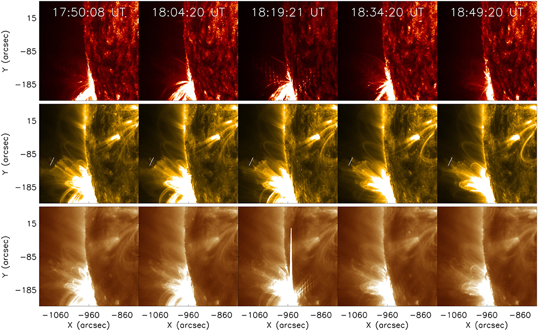
Figure 1. The evolution of the coronal loop system during the hour around the oscillations analyzed here. Plotted are the SDO/AIA 304 Å (top), 171 Å (middle), and 193 Å (bottom) channels. The white slit over-laid on the middle row indicates the location of the slit analyzed in this article.
2.2. Tracking the Loop Displacement and Model Fitting
In Figure 2, we plot a zoomed in FOV of the oscillation analyzed here for five time-steps (top row). The white line over-laid on these images indicates the location of the slit analyzed in this article. The co-ordinates of this slit are the same as for Loop 40, Event 2 included in the table of Goddard et al. (2016). This event was studied subsequently by Pascoe et al. (2016, 2017); Pagano et al. (2018). Following the construction of the time-space diagram from 171 Å images (plotted in the bottom panel of Figure 2), we applied a Canny edge-detection algorithm to obtain approximations for the coronal loop boundaries. The output for this edge detection routine is over-laid on the time-space diagram in Figure 3 (blue lines). In order to model the oscillation of the loop axis, we assumed that the displacement is guided by midpoints between the boundaries of the upper loop as shown by the red dots in Figure 3. If we assume that the loop is cylindrical and radially symmetric, then the errors associated by this fitting can be assumed to be less than 1 pixel. Understanding whether such assumptions are justified would require much higher resolution data and so should be studied in the future. As the loop axis returned through time is qualitatively similar to that plotted in Figure 1 of Pascoe et al. (2016) for the same event, in the following we assume that this oscillation profile is accurate and, therefore, neglect any further potential errors in our fitting. Ignoring any further errors introduced through the loop fitting is justified in this case, as our study aims to show, in principle, that including the effects of cooling could have important implications for coronal loop modeling. A larger statistical study conducted using a variety of fitting methods in the future will be required to fully understand the prevalence and importance of coronal loop cooling on kink-mode oscillations.
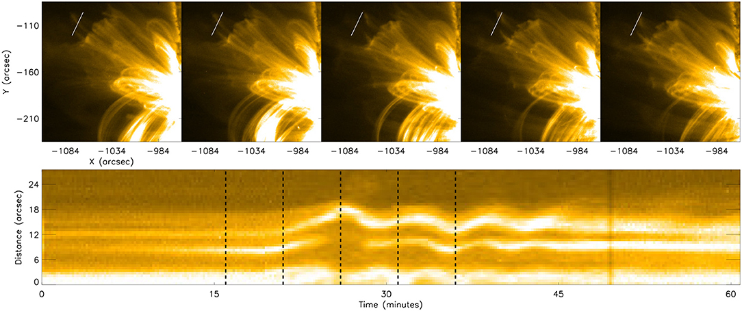
Figure 2. (Top) The coronal loop system analyzed here plotted using 171 Å data at five times during the oscillation. The white lines indicate the slit studied in this article, which corresponds to Loop 40, Event 2 from Goddard et al. (2016). (Bottom) Time-space diagram constructed from the slit over-laid on the 171 Å data. The dashed vertical lines indicates the time steps plotted in the top row (from left to right). The bright chord starting and finishing at 12′′ is the oscillation studied in this article.
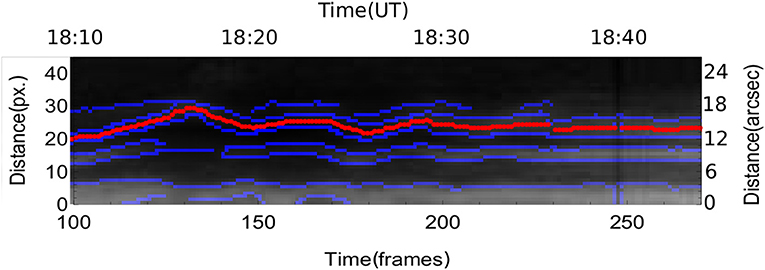
Figure 3. Zoomed time-space diagram from Figure 2 with the Canny edge-detection output (blue lines) and the returned oscillation profile (red line) over-laid. The returned oscillation is qualitatively similar to the oscillation returned by Pascoe et al. (2016) for the same event.
The oscillation extracted from this time-space diagram is plotted with red dots in Figure 4. The approximate background trend of the loop was modeled by a polynomial of the 8th degree on all obtained data points (i.e., from frame 0 to 300) and is over-laid for the region of interest (between frames 130 and 230) as the green line in Figure 4. The 8th order polynomial was selected as it best tracked the background of the amplitude profile throughout the entire time-series (including the parts where no oscillation was detected). It should be noted that a number of background trends with different orders were tested with each returning similar seismological results. This is because the ratio of the internal and external densities, which we can calculate from this model, is dependent only on where, in this case, the increment to the amplitude is (which did not change for any background trend), not how large it is. This will be discussed in further detail later in the article.
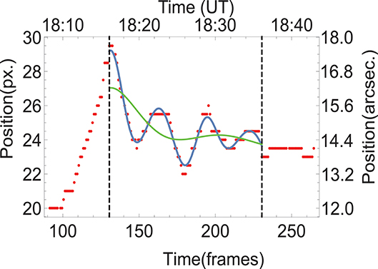
Figure 4. The position-time dependence of the coronal loop. Red dots correspond to data points collected from the 171 Å time-space diagram plotted in Figure 3. The green line corresponds to the fitted 8th-order background trend and the blue line is the Gaussian fit of the observed data points computed of the form (Equation 1). The two vertical dashed lines indicate the boundaries of the area over which numerical fitting took place. The Gaussian fit under-estimates the oscillation amplitude between frames 170 and 200 meaning the amplitude at this time will be under-estimated.
The numerical fitting of the red points is done by considering the summation of four equations of Gaussian form:
where Ai, μi, and σi are variables to be fitted for each peak, t is time (in frames), and f(amp) is the final fitted function. The benefit of such fits over a typical sinusoidal fit is that no periodicity is assumed a priori. This fitting was completed using the Wolfram Mathematica 11.3 procedure Non-linearModelFit (which guarantees continuity of the summed functions) and is plotted as the blue line over-laid on Figure 4. It is clear that this blue line accurately models the detected oscillation, however, it does slightly under-estimate the returned amplitude between frames 170 and 200. Therefore, we stress that the increase in amplitude detected during this oscillation (discussed subsequently) will be under-estimated by our model.
3. Results
3.1. Theoretical Modeling and Observed Amplitude Profiles
In this section, we fit the observed oscillatory profile plotted in Figure 4 using the theoretical model proposed by Shukhobodskiy et al. (2018). The model proposed by those authors consisted of a straight magnetic flux tube with varying cross section along its length. The tube was modeled with three layers: the core which contained an arbitrary flow and oscillated as a solid body; a transitional layer (or annulus) with monotonically decaying density from the core to the external layer; and the surrounding background plasma. See Figure 5 for a detailed schematic of this model. Ruderman et al. (2017) obtained the governing equation for such a model under the assumptions of a thin tube with thin boundaries, by considering jumps of displacement and pressure across the transitional layer. However, this equation was not closed as jump conditions were not defined in terms of the displacement. Later, Shukhobodskiy and Ruderman (2018) and Shukhobodskiy et al. (2018), closed that system for the time independent and time dependent densities, respectively.
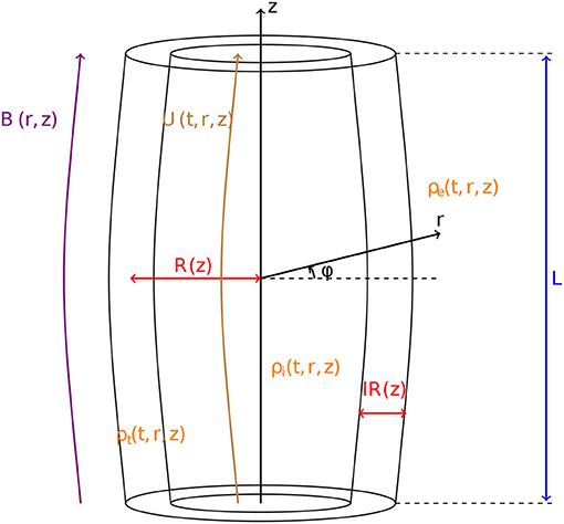
Figure 5. Equilibrium configuration of theoretical model. The black lines with labels r, ϕ, and z correspond to the cylindrical polar coordinates system. B(r, z) is the background magnetic field, U(t, r, z) is the background flow parallel to the magnetic field, R(z) is the radius of the tube, l is a constant determining the thickness of the transitional layer, ρi(t, r, z) is the density in the internal region, ρe(t, r, z) is the density in external region, ρt(t, r, z) is the monotonically decaying density in the transitional layer from ρi(t, r, z) to ρe(t, r, z), L is the length of tube for the standing waves and the characteristic value of the wavelength for propagating waves.
In the model applied here, we consider a loop of half-circular shape, where the curvature affects only the density distribution. The temperature is modeled to be exponentially decaying in time (similar to the profiles studied in, for example, Aschwanden and Terradas, 2008; Morton and Erdélyi, 2010; Ruderman, 2011a; Ruderman et al., 2017) and is approximated by:
where T0 is the constant external temperature and tcool is the cooling time (assumed to be the total lifetime of the oscillation here). Additionally, we describe the variation of the loop cross-section with height, z, in a manner similar to that discussed by Ruderman et al. (2008, 2017) and Shukhobodskiy et al. (2018). This takes the form:
where Rf is the radius of the magnetic flux tube at the foot-points, λ = R(0)/Rf is the expansion factor and Lc is an arbitrary constant. Please note that Lc should be selected such that the expansion factor can be consistent with observations of coronal loops (1 < λ < 1.5). We also assume, similarly to Ruderman and Roberts (2002) and Goossens et al. (2002), that the density in the transitional layer has a linear profile modeled by:
where l is a constant determining the width of the transition layer and ρi and ρe are the internal and external densities, respectively.
Using these equations, Shukhobodskiy et al. (2018) showed that the dimensionless amplitude, A where A(0) = 1, of the kink mode may be approximated by:
where:
and:
Here, μ0 is the magnetic permeability of the free space, ω is the oscillation frequency, H0 is the external scale height, and ρf and Bf are the density of plasma and magnetic field strength at the foot-points inside the loop. Additionally, X is determined by the following boundary value problem:
where X is the function of Z defined by the boundary values:
In order to obtain results comparable with observed amplitude profiles, we set At = A(0)AOb(0), where AOb(0) is the measured initial amplitude of the observed oscillation, At is the factor by which the dimensionless amplitude is scaled, and set L/Lc = 6 (similar to the values used by Ruderman et al., 2008, 2017; Shukhobodskiy et al., 2018). This allows us to obtain results for loop expansion factors in the range of 1–1.5, consistent with values discussed in the literature for coronal loops (see for example, Klimchuk, 2000; Watko and Klimchuk, 2000). In Figure 6, we plot the absolute displacement of the observed oscillation through time by subtracting the fitted displacement (blue line in Figure 4) from the background trend (green line in Figure 4). We define the initial amplitude of the oscillation, AOb(0), by the first peak in Figure 6. The observed amplitude profile is then constructed by calculating all values of the peaks in Figure 6 and using the Interpolation procedure in Wolfram Mathematica 11.3.
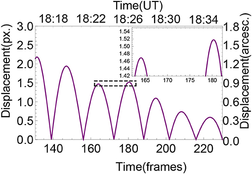
Figure 6. The absolute value of the displacement of the Gaussian fitted position profile (blue line from Figure 4) from the background 8th order polynomial trend (green line from Figure 4) through time. The cut-out in the top right corner provides a magnified view of the region on the graph bounded by the black dashed box. This cut-out clearly shows the deviation of the damping profile from a typical Gaussian or exponential fit during this time due to a slight increase in the measured amplitude (compared to the background trend). Similar results are found for other background polynomial trends.
The most interesting region of Figure 6 (denoted by the dashed black box over-laid between frames 160 and 185) is plotted in the zoomed cut-out in the top right corner of the panel. It is immediately clear that peak four is slightly larger than peak three indicating an amplitude increase potentially occurs through time. Such an increase would be in agreement with the theoretical model of Shukhobodskiy et al. (2018) which suggests that cooling in the loop system can lead to wave amplification. We note that cooling does not strictly lead to an amplification of the oscillation, it only modifies the damping profile from Gaussian or exponential. Therefore, although the amplitude increase plotted here is sub-resolution, the fact that the oscillation is not damping in a manner consistent with a Gaussian or exponential profile is enough to suggest some sort of cooling may be occurring. It should also be noted that larger amplitude increases (greater than 1 pixel) were found for lower order polynomials, however, we only focus on the 8th order fitting here as that is sufficient as a proof of concept. The increase in the amplitude can be clearly seen in Figure 7, where the blue line plots a fit between the measured peak amplitudes (green circles) through time. The red line over-laid on Figure 7 indicates the line of best fit calculated by solving the system of Equations (2–10) numerically. A maximum χ2 value was found by looping over all variables, hence this is numerically expensive. It was assumed that the cooling starts at the first peak and ends in the last peak of Figure 6 (i.e., that tcool is equal to the lifetime of the oscillation).
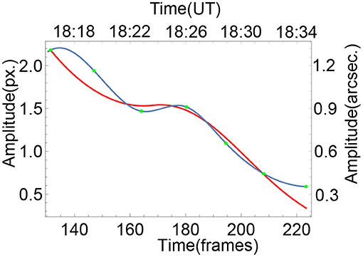
Figure 7. The dependence of the amplitude of the coronal loop oscillation on time. Green points correspond to maxima of the peaks plotted in Figure 6, the blue line is the fitted observed amplitude-time profile, and the red line represents the theoretical amplitude-time profile with ζ = 2.2, λ = 1.05, κ = 2.4, and α = 1.4.
The software used to obtain these theoretical solution is Wolfram Mathematica 11.3. The numerical procedure for obtaining the theoretical results may be summarized as follows: To obtain the solution to the boundary value problem, Equations (9) and (10), we used the NDEigensystem procedure; Equation (6) was then integrated numerically using the NIntegrate procedure subject to the GlobalAdaptive method (which uses various numerical integration methods and chooses the most accurate and fastest version for the particular problem). Finally we obtained the amplitude of the oscillation by using the NDSolve procedure.
The application of this model revealed several interesting effects with regards seismology of the loop system. Firstly, it was found that ζ (the density ratio at the foot-points of the loop at t = 0) and κ (the scale height) determine the position of the turning points of the amplitude profile (i.e., where the gradient of the amplitude profile is zero). However, the effect of κ on the position of the turning point reduces as the value of κ itself increases. As a result, we can neglect this effect for sufficiently long loops with κ > 1.6. Therefore, by minimizing the difference between the turning points of the theoretical and observed amplitude profiles we can determine an approximate value of ζ for this system without knowing any other background parameters. For the example studied here, fitting a density ratio of between 2.05 and 2.35 provides sufficiently good approximations for the position of the local amplitude increase. As this work aims to provide a proof-of-concept of the application of cooling theory to coronal loop oscillations and as the density ratio is only dependent on where the amplitude deviates from a Gaussian or exponential decay, we neglect any errors in the measured amplitude (green dots) here; however, the effects of any errors on our seismological should be analyzed using a larger statistical sample in the future. The differences in nature between the red and blue curves are due to the spline fitting used here. Secondly, the values of κ, α, and λ determine the speed of the amplitude decay. Unfortunately, for the example studied here, various sets of these parameters return similar shapes and amplitude profiles meaning we are unable to provide accurate seismological estimates at this stage. A larger statistical sample of cooling events and further numerical work will be required to attempt to estimate such values in the future.
3.2. Evidence for Cooling in the AR
Evidence of cooling in the coronal loop system can be inferred through analysis of the intensities within SDO/AIA imaging channels. For the loop studied here, no evidence of coronal rain formation was found in the 304 Å filter indicating that catastrophic cooling likely did not take place within this loop. The loop intensity within the 171 Å and 193 Å filters did appear to decrease slightly (potentially below any level of significance) during the oscillation, however, whether this was due to cooling, some line-of-sight effects (e.g., the supposition of multiple loops within one pixel), or purely noise is unknown. The flare within the local AR lead to large swathes of saturation and fringing patterns on the 193 Å data meaning we were unable to study the temporal evolution of the loop in detail in this wavelength during the period of interest for cooling for this event. Future work should aim to analyse a larger statistical sample of coronal loop oscillations with non-Gaussian and non-exponential damping profiles in order to detect whether direct signatures of cooling can be found within the loops themselves.
Significant cooling can be inferred elsewhere in this AR during the course of this oscillation, however. Large amounts of coronal rain can be observed in the 304 Å channel in the loop system approximately 100′′ south of the loop analyzed here potentially indicating the occurrence of the thermal instability during the flare. The after-effects of this rain are evident in the top row of Figure 1 (at approximately xc = −200′′, yc = −990′′). Initially (at 17:50 UT), the loop is bright in the 304 Å channel. As the rain forms, the loop system completely fades from view (by 18:50 UT). The coronal rain in the chromospheric 304 Å channel is accompanied by a reduction in the intensity of the loop system in the coronal 171 Å and 193 Å channels further supporting the hypothesis that cooling occurred. The application of the theories tested here on loops which are catastrophically cooling would be an interesting project for the future.
4. Discussion and Conclusions
In this article, we have studied a flare-driven kink oscillation in a coronal loop observed in AR 11598 by the SDO/AIA instrument (Figure 1). This oscillation corresponded to Loop 40, Event 2 from Goddard et al. (2016). The specific slit analyzed here is indicated by the white line over-laid on the top row of Figure 2, with the returned time-space diagram being plotted in the bottom panel of Figure 2. In Figure 3 the time-space diagram is plotted with the output from a Canny edge-detection algorithm over-laid in blue. The mid-points between the edge-detection outputs (red dots) were assumed to track the displacement of the center of the loop as it oscillated. The returned oscillation was qualitatively similar to that returned by Pascoe et al. (2016) for the same event indicating that our fitting method was sound. This oscillation was then fitted with a summation of four Gaussian functions (corresponding to the four peaks in the oscillation) of the form Equation 1 and an 8-th order background trend removed (the blue and green lines in Figure 4, respectively). Again, it should be emphasized that numerous background trends were tested in order to assure that we were not introducing important effects in our subsequent analysis.
Once the oscillation and the background had been fitted, we removed the background trend from the oscillation and plotted the absolute values of the kink mode (see Figure 6) through time. The cut-out over-laid on Figure 6 clearly highlights a deviation in oscillatory amplitude from a typical Gaussian or exponential damping between frames 160 and 185 (18:22 UT – 18:27 UT). Indeed, there are even hints that an amplitude increase could be present, however, this is small. It should be noted that some background trends returned profiles with amplitude increases of over 1 pixel. Such an amplitude increase would obviously not be expected from a typical Gaussian or exponential decay (as has been considered previously by, for example, Goddard et al., 2016; Pascoe et al., 2016). However, models proposed by Shukhobodskiy and Ruderman (2018) and Shukhobodskiy et al. (2018) which consider cooling within the system can account for amplitude increases. Therefore, in addition to the multiple harmonics scenario suggested by Pascoe et al. (2017), future work should consider cooling when trying to understand complex amplitude profiles in coronal loop oscillations.
Although there were some hints that the loop faded slightly in the coronal 171 Å and 193 Å channels over the course of the hour-long dataset analyzed here, it is unclear whether this is an effect of cooling, due to line-of-sight effects, or purely noise. Little other evidence for cooling could be obtained through analysis of SDO/AIA time-series. Additionally, no evidence of coronal rain was observed in the 304 Å channel. More obvious cooling could be observed within the local AR, however, in a loop system located approximately 100′′ south of the loop analyzed here. This loop contains large amounts of coronal rain in the 304 Å channel potentially hinting at the occurrence of the thermal instability, or catastrophic cooling. The effects of such catastrophic cooling on coronal loop oscillations would be an interesting topic for future study.
The key seismological result obtained here is that the location in time at which the amplitude begins to increase (an effect of the cooling on the oscillation) is dictated solely by the ratio between the internal and external densities for sufficiently large coronal loops. Therefore, fitting the model such that the difference between the observed turning point and the theoretical fitting point is minimized (as is shown in Figure 7) allows us to calculate an estimate of the density ratio, ζ, an important parameter for modeling. For this loop, inversions of the theoretical model provide a good fit to the observed amplitude profiles when ζ is in the range 2.05–2.35 (i.e., the loop foot-point is initially more than twice as dense as its surroundings).
In order to follow on from this work, we aim to complete two further studies. Firstly, we will conduct a statistical analysis of oscillations within potentially cooling coronal loops in the solar corona. This will provide important constraints on density ratios of loops for future modeling. Secondly, through further numerical work, it should prove possible to conduct further seismology in order to return values such as the scale height of the loop and the annulus thickness. These values will, again, provide further constraints for future modeling. Overall, the theoretical work of Shukhobodskiy et al. (2018) has proved adept at modeling the oscillations of the loop analyzed here and should be considered by authors in the future when analysing coronal loop oscillations.
Author Contributions
CN drafted the manuscript and lead the observational analysis with help from AS. AS drafted section Theoretical Modeling and Observed Amplitude Profiles and completed the theoretical work. AS and CN completed the model fitting. All authors contributed to the interpretation of the results and helped draft the manuscript.
Funding
The authors acknowledge the Science and Technology Facilities Council (STFC) for financial support (Grant numbers: ST/M000826/1 and ST/P000304/1).
Conflict of Interest Statement
The authors declare that the research was conducted in the absence of any commercial or financial relationships that could be construed as a potential conflict of interest.
The reviewer RO declared a past co-authorship with one of the authors CN to the handling editor.
Acknowledgments
SDO data are courtesy of NASA/SDO and the AIA and HMI science teams.
References
Al-Ghafri, K. S., and Erdélyi, R. (2013). Effect of variable background on an oscillating hot coronal loop. Solar Phys. 283, 413–428. doi: 10.1007/s11207-013-0225-8
Antolin, P., Vissers, G., Pereira, T. M. D., Rouppe van der Voort, L., and Scullion, E. (2015). The multithermal and multi-stranded nature of coronal rain. Astrophys. J. 806:81. doi: 10.1088/0004-637X/806/1/81
Aschwanden, M. J., Fletcher, L., Schrijver, C. J., and Alexander, D. (1999). Coronal loop oscillations observed with the transition region and coronal explorer. Astrophys. J. 520, 880–894. doi: 10.1086/307502
Aschwanden, M. J., and Terradas, J. (2008). The effect of radiative cooling on coronal loop oscillations. Astrophys. J. Lett. 686:L127. doi: 10.1086/592963
Dymova, M. V., and Ruderman, M. S. (2005). Non-axisymmetric oscillations of thin prominence fibrils. Solar Phys. 229, 79–94. doi: 10.1007/s11207-005-5002-x
Dymova, M. V., and Ruderman, M. S. (2006). Resonantly damped oscillations of longitudinally stratified coronal loops. Astron. Astrophys. 457, 1059–1070. doi: 10.1051/0004-6361:20065051
Erdélyi, R., Hague, A., and Nelson, C. J. (2014). Effects of stratification and flows on P 1/ P 2 ratios and anti-node shifts within closed loop structures. Solar Phys. 289, 167–182. doi: 10.1007/s11207-013-0344-2
Goddard, C. R., Nisticò, G., Nakariakov, V. M., and Zimovets, I. V. (2016). A statistical study of decaying kink oscillations detected using SDO/AIA. Astron. Astrophys. 585:A137. doi: 10.1051/0004-6361/201527341
Goossens, M., Andries, J., and Aschwanden, M. J. (2002). Coronal loop oscillations. An interpretation in terms of resonant absorption of quasi-mode kink oscillations. Astron. Astrophys. 394, L39–L42. doi: 10.1051/0004-6361:20021378
Handy, B. N., Acton, L. W., Kankelborg, C. C., Wolfson, C. J., Akin, D. J., Bruner, M. E., et al. (1999). The transition region and coronal explorer. Solar Phys. 187, 229–260. doi: 10.1023/A:1005166902804
Klimchuk, J. A. (2000). Cross-sectional properties of coronal loops. Solar Phys. 193, 53–75. doi: 10.1007/978-94-010-0860-0_4
Lemen, J. R., Title, A. M., Akin, D. J., Boerner, P. F., Chou, C., Drake, J. F., et al. (2012). The Atmospheric Imaging Assembly (AIA) on the Solar Dynamics Observatory (SDO). Solar Phys. 275, 17–40. doi: 10.1007/s11207-011-9776-8
López Fuentes, M. C., Klimchuk, J. A., and Mandrini, C. H. (2007). The temporal evolution of coronal loops observed by GOES SXI. Astrophys. J. 657, 1127–1136. doi: 10.1086/510662
Morton, R. J., and Erdélyi, R. (2009). Transverse oscillations of a cooling coronal loop. Astrophys. J. 707, 750–760. doi: 10.1088/0004-637X/707/1/750
Morton, R. J., and Erdélyi, R. (2010). Application of the theory of damping of kink oscillations by radiative cooling of coronal loop plasma. Astron. Astrophys. 519:A43. doi: 10.1051/0004-6361/201014504
Nakariakov, V. M., Ofman, L., Deluca, E. E., Roberts, B., and Davila, J. M. (1999). TRACE observation of damped coronal loop oscillations: implications for coronal heating. Science 285, 862–864. doi: 10.1126/science.285.5429.862
Pagano, P., Pascoe, D. J., and De Moortel, I. (2018). Contribution of phase-mixing of Alfvén waves to coronal heating in multi-harmonic loop oscillations. Astron. Astrophys. 616:A125. doi: 10.1051/0004-6361/201732251
Pascoe, D. J., Goddard, C. R., Nisticò, G., Anfinogentov, S., and Nakariakov, V. M. (2016). Damping profile of standing kink oscillations observed by SDO/AIA. Astron. Astrophys. 585:L6. doi: 10.1051/0004-6361/201527835
Pascoe, D. J., Russell, A. J. B., Anfinogentov, S. A., Simões, P. J. A., Goddard, C. R., Nakariakov, V. M., et al. (2017). Seismology of contracting and expanding coronal loops using damping of kink oscillations by mode coupling. Astron. Astrophys. 607:A8. doi: 10.1051/0004-6361/201730915
Ruderman, M. S. (2011a). Resonant damping of kink oscillations of cooling coronal magnetic loops. Astron. Astrophys. 534:A78. doi: 10.1051/0004-6361/201117416
Ruderman, M. S. (2011b). Transverse oscillations of coronal loops with slowly changing density. Solar Phys. 271, 41–54. doi: 10.1007/s11207-011-9772-z
Ruderman, M. S., and Roberts, B. (2002). The damping of coronal loop oscillations. Astrophys. J. 577, 475–486. doi: 10.1086/342130
Ruderman, M. S., Shukhobodskiy, A. A., and Erdélyi, R. (2017). Kink oscillations of cooling coronal loops with variable cross-section. Astron. Astrophys. 602:A50. doi: 10.1051/0004-6361/201630162
Ruderman, M. S., Verth, G., and Erdélyi, R. (2008). Transverse oscillations of longitudinally stratified coronal loops with variable cross section. Astrophys. J. 686, 694–700. doi: 10.1086/591444
Shukhobodskiy, A. A., and Ruderman, M. S. (2018). Resonant damping of kink oscillations of thin expanding magnetic tubes. Astron. Astrophys. 615:A156. doi: 10.1051/0004-6361/201732396
Shukhobodskiy, A. A., Ruderman, M. S., and Erdélyi, R. (2018). Resonant damping of kink oscillations of thin cooling and expanding coronal magnetic loops. Astron. Astrophys. 619:A173. doi: 10.1051/0004-6361/201833714
Watko, J. A., and Klimchuk, J. A. (2000). Width Variations along Coronal Loops Observed by TRACE. Solar Phys. 193, 77–92. doi: 10.1007/978-94-010-0860-0_5
Winebarger, A. R., and Warren, H. P. (2005). Cooling active region loops observed with SXT and TRACE. Astrophys. J. 626, 543–550. doi: 10.1086/429817
Keywords: solar corona, coronal loop oscillations, magnetohydrodynamics, kink oscillations, cooling
Citation: Nelson CJ, Shukhobodskiy AA, Erdélyi R and Mathioudakis M (2019) The Effect of Cooling on Driven Kink Oscillations of Coronal Loops. Front. Astron. Space Sci. 6:45. doi: 10.3389/fspas.2019.00045
Received: 18 January 2019; Accepted: 27 May 2019;
Published: 27 June 2019.
Edited by:
Patrick Antolin, University of St. Andrews, United KingdomReviewed by:
Petra Kohutova, University of Oslo, NorwayVaibhav Pant, KU Leuven, Belgium
Ramon Oliver, University of the Balearic Islands, Spain
Copyright © 2019 Nelson, Shukhobodskiy, Erdélyi and Mathioudakis. This is an open-access article distributed under the terms of the Creative Commons Attribution License (CC BY). The use, distribution or reproduction in other forums is permitted, provided the original author(s) and the copyright owner(s) are credited and that the original publication in this journal is cited, in accordance with accepted academic practice. No use, distribution or reproduction is permitted which does not comply with these terms.
*Correspondence: Chris J. Nelson, Yy5qLm5lbHNvbkBzaGVmZmllbGQuYWMudWs=