 Swayamtrupta Panda1,2*
 Mary Loli Martínez-Aldama1
 Michal Zajaček1 on behalf of the LSST AGN Science Collaboration
- 1Center for Theoretical Physics, Polish Academy of Sciences, Warsaw, Poland
- 2Nicolaus Copernicus Astronomical Center, Polish Academy of Sciences, Warsaw, Poland
Reverberation mapping technique (RM) is an important milestone that has elevated our understanding of Active Galactic Nuclei (AGN) demographics, giving information about the kinematics and the structure of the Broad Line Region (BLR). It is based on the time-delay response between the continuum and the emission line. The time delay is directly related to the size of the BLR which in turn is related to the continuum luminosity of the source, producing the well-known Radius-Luminosity (RL) relation. The majority of the sources with RM data, have been monitored for their Hβ emission line in low redshift sources (z < 0.1), while there are some attempts using the Mg II line for higher redshift ranges. In this work, we present a recent Mg II monitoring for the quasar CTS C30.10 (z = 0.90) observed with the 10-m Southern African Large Telescope (SALT), for which the RL scaling based on Mg II holds within measurement and time-delay uncertainties. One of the most important advantages of reverberation mapping technique is the independent determination to the distant source, and considering the large range of redshifts and luminosities found in AGNs their use in cosmological studies is promising. However, recently it has been found that highly accreting sources show the time delays shorter than expected from the RL relation. We have proposed a correction for this effect using a sample of 117 Hβ reverberating-mapped AGN with 0.02 < z < 0.9, which recovers the low scatter along with the relation. We are able to determine the cosmological constants, Ωm and ΩΛ. Despite the applied correction, the scatter is still large for being effective for cosmological applications. In the near future, Large Synoptic Survey Telescope (LSST)1 will cover over 10 million quasars in six photometric bands during its 10-years run. We present the first step in modeling of light curves for Hβ and Mg II and discuss the quasar selection in the context of photometric reverberation mapping with LSST. With the onset of the LSST era, we expect a huge rise in the overall quasar counts and redshift range covered (z ≲ 7.0), which will provide a better constraint of AGN properties with cosmological purposes.
1. Introduction
Reverberation mapping (hereafter RM) is a robust observational technique to determine the time-lag τ0 between the variability of the ionizing continuum of an active galactic nucleus (AGN) and the line emission associated with the broad-line region (BLR, Blandford and McKee, 1982). This is only possible since the emission-line flux densities are highly correlated with the continuum flux, which implies that the AGN continuum related to the power generated by the accretion disk is the main source of photoionization. The main source of recombination emission lines is the BLR material, that is optically thick with respect to the ionizing UV/optical continuum.
The first straightforward application of RM is to determine the size of the BLR, RBLR = cτ0 (see e.g., Netzer and Peterson, 1997; Kaspi et al., 2000; Peterson et al., 2004; Mejía-Restrepo et al., 2018).
The second application combines τ0 and the line width of the broad emission line. It can be considered that the large line width of the BLR gas ΔvFWHM2 of several thousand km/s, is due to the Doppler broadening of clouds that are gravitationally bound to the supermassive black hole (SMBH). The 3D Keplerian velocity of the gas vBLR = fvirΔvFWHM can be inferred, though it depends on the rather uncertain virial factor fvir. By combining these two pieces of information, one can estimate the virial black hole mass,
where the virial factor fvir is of the order of unity and depends on the overall geometrical distribution of the BLR clouds, their kinematics as well as their line of sight emission properties, c is the velocity of light and G is the Gravitational constant. The virial factor mainly depends on the inclination i of the BLR plane with respect to the observer and the thickness of the BLR, HBLR/RBLR, and can be expressed as (Collin et al., 2006; Mejía-Restrepo et al., 2018; Panda et al., 2019),
Therefore, the virial factor dependence on the viewing angle of the BLR and its geometrical properties, introduces an overall uncertainty in the virial mass determination. Fixing the virial factor to a constant value, which is frequently applied to single-epoch measurements (Woo et al., 2015), can lead to a virial-mass difference of a factor of 2–3 (Mejía-Restrepo et al., 2018). Comparing the black hole mass estimations determined from the spectral energy distribution (SED) fitting of the AGN continuum, with the viral black hole mass, Mejía-Restrepo et al. (2018) found that the virial factor is inversely proportional to the FWHM of the broad lines, . This could be interpreted as the effect of the BLR viewing angle (inclination) or as the effect of the radiation pressure on the BLR distribution. The strong effect of the BLR inclination directly results from the plane-like geometry of the BLR, in which the BLR consists of cloudlets that have an overall flattened geometry (Gaskell, 2009). This “nest-like” model of the BLR is also consistent with the first direct velocity-resolved observation of the BLR in 3C273 (Gravity Collaboration et al., 2018) using the Very Large Telescope Interferometer GRAVITY at the European Southern Observatory (Gravity Collaboration et al., 2017). The flattened geometry of the BLR that follows the disc geometry could be explained by the formation of the BLR clouds from the disc material beyond the dust sublimation radius (Czerny and Hryniewicz, 2011). The radiation pressure acting on the dust in the BLR clouds then leads to their lift-off from the disc plane and subsequent fall-back when the dust evaporates. This is one possible scenario for the origin of the low-ionization line component of the BLR (LIL), so-called failed radiatively accelerated disc outflow (FRADO, Czerny et al., 2017), while the high-ionization line (HIL) component seems to be associated with nuclear outflows (Collin-Souffrin et al., 1988).
Finally, the third application of the RM is the power-law radius–luminosity relation between the BLR radius (or time-delay) and the AGN monochromatic optical luminosity. Initially, Kaspi et al. (2005) found the slope α = 0.67 ± 0.05 between the optical monochromatic luminosity and the broad Hβ line, which implied a deviation from simple theoretical models predicting a slope of 0.5. The relation was further modified for lower-redshift sources using the Hβ RM and the luminosity at 5,100 (Bentz et al., 2006, 2009, 2013) taking into account the host galaxy starlight. After the removal of the host-galaxy starlight from the total luminosity, the power-law slope was determined to be (Bentz et al., 2013), which is consistent with the theoretical expectation from simple photoionization models. The slope of α = 1/2 simply follows from the ionization parameter of a BLR cloud, , where R is the cloud distance from an ionizing continuum, c is the speed of light, nH is the number density, and is the ionizing photon flux. In general, one can assume that the ionization conditions as well as the gas density in the BLR are comparable for all AGN, i.e., the product UnH is constant, from which follows (Netzer, 2013).
In Figure 1 the RHβ − L5100 relation created from 117 Hβ reverberation-mapped AGN. The full sample consists of 48 sources previously monitored by Bentz et al. (2009, 2014), Barth et al. (2013), Pei et al. (2014), Bentz et al. (2016), and Fausnaugh et al. (2017), 25 super-Eddington sources of the SEAMBH project (Super-Eddington Accreting Massive Black Holes, Wang et al., 2014a; Du et al., 2015, 2016, 2018; Hu et al., 2015), 44 sources from the SDSS-RM (Grier et al., 2017) sample, and the recent monitoring for NGC5548 (Lu et al., 2016) and 3C273 (Zhang et al., 2019). See more details concerning the sample in Martínez-Aldama et al. (2019a).
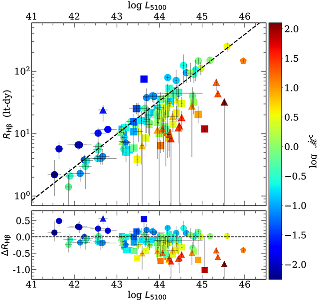
Figure 1. (Top) RHβ − L5100 relation for SEAMBH (triangles), SDSS-RM (squares), Bentz Collection (circles), NGC5548, and 3C 273 (pentagons). (Bottom) Difference between the BLR size estimated from the observed time delay and the predicted ones by the RL relation (black line, Equation 1). In both panels, colors indicate the variation in dimensionless accretion rate, .
The importance of the RHβ − L5100 relationship lies in the fact that it is the basis of secondary black-hole mass estimates, especially for high-z AGN (Laor, 1998; Wandel et al., 1999; McLure and Jarvis, 2002; Vestergaard and Peterson, 2006). In principle, by knowing the optical luminosity of the source, one can infer the black-hole mass from a single-epoch spectrum (by extracting the broad-line FWHM), which makes it especially useful for large statistical surveys of sources throughout the cosmic history. Given the importance of RHβ − L5100 relation, it is necessary to verify it using different emission lines from the LIL BLR region and higher-redshift sources, which we will analyze in subsequent section for the case of MgII line and the redshift of 0.9 (a complete and updated MgII based RM sample is reported in Zajaček et al. 2019, submitted to Astrophysics Journal).
RM of quasars, using both the BLR reverberation technique and the accretion disc radiation reprocessing, was suggested to be utilized in cosmological studies (Collier et al., 1999; Elvis and Karovska, 2002; Horne et al., 2003). In particular, the RHβ − L5100 relation directly enables to turn reverberation-mapped quasars into “standardizable” luminosity candles (Haas et al., 2011; Watson et al., 2011; Bentz et al., 2013; Czerny et al., 2013). Under the assumption that the RHβ − L5100 power-law relationship applies not only to Hβ line but also other LIL lines, one could apply it to intermediate- and high-redshift quasars whose co-moving time-delay was determined to infer their absolute luminosities. From measured monochromatic flux densities of the sources, one can infer the luminosity distance and the Hubble diagram of reverberation-mapped quasars. The critical point here is to reduce the scatter along the radius-luminosity relation, both by improving the RM time-lag precision and by correctly subtracting the host starlight (Haas et al., 2011).
The paper is structured as follows. In section 2, we report on the detection of MgII line time-delay for the intermediate-redshift quasar CTS C30.10 and its consistency with the radius-luminosity relation previously derived for Hβ emission in lower redshift sources. We continue with section 3 to analyze in detail how accretion rate affects the position of sources along the RHβ − L5100 relation. We summarize the initial cosmological constraints as derived from the current reverberation-mapped quasar sample in section 4. First steps of modeling stochastic lightcurves in the context of reverberation mapping with the Large Synoptic Survey Telescope (LSST) are analyzed highlighting a novel filtering algorithm to select higher quality photometric data in section 5. We discuss a few open problems in section 6 and finally conclude with section 7.
2. Radius-Luminosity Relationship Toward Higher Redshifts: Time-Lag Determination of MgII Response in CTS C30.10
Previously the power-law radius-luminosity relation, , was observationally constrained using Hβ broad line for low-redshift sources up to z = 0.292 (Kaspi et al., 2000; Bentz et al., 2009, 2013), with the scatter as low as 0.13 dex and the power-law index of (Bentz et al., 2013) after the host starlight correction. The analysis using Hβ broad line limits the redshift of the sources up to z ~ 0.6 for optical observations with the maximum wavelength limit of 8,000 Å. However, other LIL broad lines can extend the redshift range to intermediate values. MgII line with the rest wavelength~2798 Å is suitable for the reverberation-mapping studies in the redshift range z = 0.4 − 1.5 for ground based telescopes, which is also utilized for the sample of seven objects monitored by the South African Large Telescope (SALT) telescope (Czerny et al., 2013).
Between December 6, 2012 and December 10, 2018, we monitored the quasar CTS C30.10 using the 10-meter SALT telescope in order to detect the time-lag of the LIL emission-line of MgII with respect to the quasar continuum. The hypothesis was to probe the consistency of the radius-monochromatic luminosity relation toward higher redshifts and higher absolute luminosities. The quasar CTS C30.10 was discovered as a bright source in the Calan-Tololo survey (Maza et al., 1993) among 200 newly discovered quasars with the visual magnitude of V = 17.2 (NED) at the intermediate redshift of z = 0.90052 (Modzelewska et al., 2014). The equatorial coordinates of the source are RA = 04 h 47 m 19.9 s and Dec = −45 d 37 m 38 s (J2000.0).
The MgII emission-line light curve was constructed based on the long-slit spectroscopy mode of the SALT telescope with the slit width of 2″ (for details, see Modzelewska et al., 2014; Czerny et al., 2019). The MgII line was extracted from the spectral energy distribution of CTS C30.10 in the wavelength range 2,700−2,900 by subtracting the two spectral components, namely the power-law component due to the accretion disc thermal emission, and FeII—line pseudo-continuum. The MgII broad line was found to consist of two kinematic components—redshifted and blueshifted Lorentzian profiles3—each of which further consists of a doublet at 2796.35 and 2803.53 with the doublet ratio of 1.6. The equivalent width (EW) of the MgII line, EW ~ Fline/Fcont, was calculated by numerical integration of all four spectral components—two kinematic and two doublet components. Because of the two kinematic components of MgII line, CTS C30.10 belongs to type B quasars (Sulentic et al., 2007; Modzelewska et al., 2014) characterized by lower Eddington ratios in the range log(L/LEdd) = 0.01−0.2 (Sulentic et al., 2011), while type A sources exhibit a single component MgII line of a Lorentzian shape (Laor et al., 1997; Véron-Cetty et al., 2001; Sulentic et al., 2002, 2009, 2011; Zamfir et al., 2010; Shapovalova et al., 2012). The origin of two components is still quite uncertain although the presence of the second, asymmetric component and the overall FWHM is consistent with our source belonging to Pop. B. It could either imply the presence of second emission region due to absorption or scattering or it could hint at the origin of LIL lines close to the disc plane, resembling thus the disc kinematics, which would naturally lead to two components when viewed off-axis.
The continuum light curve was obtained from the OGLE-IV survey in the V-band and SALTICAM in the g-band. The SALTICAM observations were shifted freely to match the overlapping V-band values. Since the SALT observations are not spectrophotometric, MgII flux density was obtained using its EW and the continuum flux density.
The normalized continuum dispersion was 6.0%, while the line dispersion was 5.2%, which is slightly lower but comparable within uncertainties. This is consistent with the simple reprocessing scenario, where the central disc provides all the ionizing UV photons which are absorbed and scattered by BLR clouds at larger distances. This allowed us to use both the continuum and the line-emission light curves to infer the time-delay τMgII of the MgII broad line.
2.1. Time-Lag Determination of MgII Line Using Cross-Correlation Function
First, we used the standard interpolated cross-correlation function (ICCF) to infer the time-delay between the MgII line-emission and the V-band continuum, which corresponds to the continuum around the redshifted MgII line. The ICCT requires regularly sampled datasets, while realistic light curves are unevenly sampled. The regular timestep is achieved by interpolating the continuum light curve to time-shifted emission-line light curve or vice versa. Typically, both interpolations are averaged to obtain the symmetric ICCF. Given the two light curves xi and yi sampled at discrete time intervals ti (i = 1, …,N) with the regular time-step Δt = ti+1 − ti, we can define the cross-correlation function (CCF) as,
where and are light curve mean values, respectively, and τk = kΔt (k = 0, …,N − 1) is the time-shift of the second light curve with respect to the first one at which the CCF is evaluated.
We make use of the PYTHON code PYCCF (Sun et al., 2018), which is the implementation of earlier CCF analysis by Gaskell and Peterson (1987) and Peterson et al. (1998). We calculate CCF separately for interpolated continuum, interpolated emission-line curves as well as the symmetric case. Using thousand Monte Carlo runs of the combined random subset selection (RSS) and flux randomization (FR), we obtain distributions of the CCF centroid (CCFC) and the CCF peak (CCFP), from which we can calculate the corresponding uncertainties, see Figure 2.
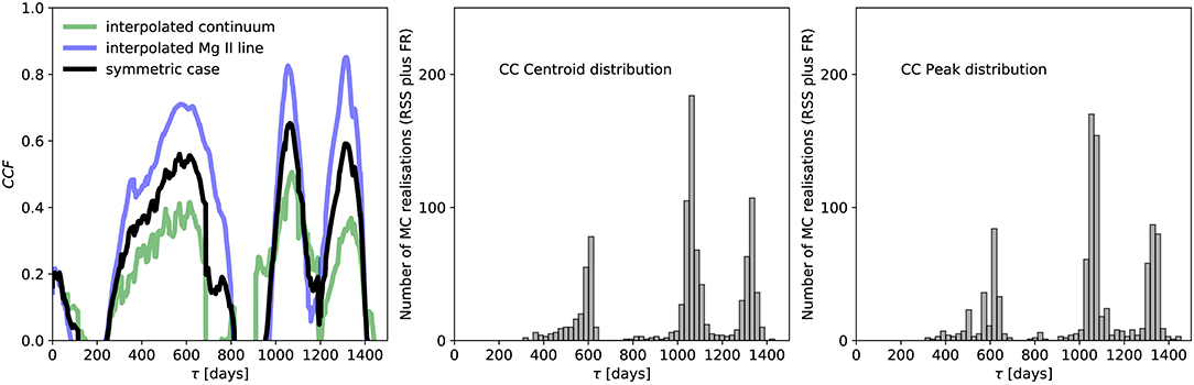
Figure 2. Results of the interpolated cross-correlation analysis between the continuum and MgII line emission. (Left) The CCF value as a function of the time-delay for the continuum light curve interpolated to the emission-line light curve (green line), for the emission-line light curve interpolated to the continuum light curve (blue line), and the symmetric interpolation (black line). (Middle) Cross-correlation centroid distribution. (Right) Cross-correlation peak distribution.
In Table 1, we summarize the time-delay results for all considered cases—the time-delay values are expressed with respect to the observer's frame (τobserver = (1 + z) × τrest). For the symmetric interpolation, the centroid time-delay is days. In general, the cross-correlation centroid and peak distributions have three peaks, see Figure 2, while the peak at ~1,060 is the most prominent. At this value, ICCF also reaches the largest value for the symmetric and interpolated-continuum cases, see Figure 2 (left panel), while the interpolated-line case peaks at larger time-delays. This offset may be due to the fact that the line-emission dataset is not so densely covered as the continuum light curve, which leads to artifacts when interpolating it to denser continuum light curve.
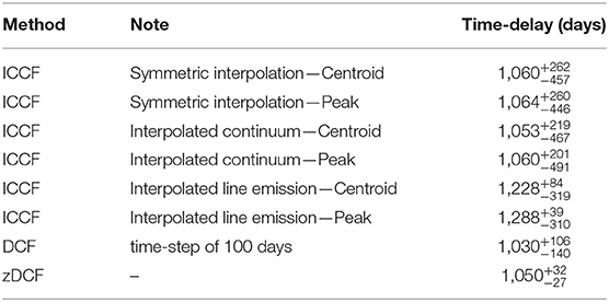
Table 1. Summary of methods used for calculating the time-delays for the quasar and their uncertainties expressed with respect to the observer's frame.
Second, we applied the discrete correlation function (DCF), which does not interpolate between the light curves and is thus better suited for unevenly sampled datasets with known measurement errors. The DCF was described by Edelson and Krolik (1988) and applied routinely to search for light curve correlations and time-lags. The first step in the DCF analysis is to look for data pairs (xi, yj) that fall into the time-delay bin of τ − δτ/2 ≤ δtji ≤ τ + δτ/2, where τ is the given time-delay, δτ is the time-delay bin and δtji = tj − ti. Given M such data pairs, one calculates a corresponding number of unbinned discrete correlation coefficients UDCFij in the following way,
where are the light curve means for a given time-delay bin. Other parameters sx and sy stand for the variances, and and are the mean measurement errors for a given time-delay bin. Subsequently, the DCF coefficient can be calculated for a given time-lag bin by averaging in total M values,
where, M is the number of light curve pairs that fall into a particular time-lag bin. The uncertainty can be estimated by the relation,
We applied the PYTHON code of Damien Robertson (see Robertson et al., 2015, for the code implementation), which calculates the DCF with the possibility of Gaussian weighting for the matching pairs of light curve points. The code allows us to select a different size for equal time-bins as well as the searched interval for the time-delay. We expand the possibilities of the code by adding the bootstrap technique to assess the significance of individual DCF peaks and to better estimate their uncertainties.
The DCF uses equal time-step binning and it is thus quite sensitive with respect to the time-bin size. We test this using three different timesteps—50, 70, and 100 days—which leads to the decrease in the mean DCF values for the time-delay at ~1,275 days, which is the most prominent for the smaller time-bins but significantly gets smaller for larger time-bins, see Figure 3 (left panel). For the time-bin size of 100 days, the largest DCF of 0.62 is for 1,050 days, followed by the peak at 550 days. Moreover, we verify the significance of individual peaks by running 1,000 bootstrap realizations where we randomly create subsamples from both light curves simultaneously. We obtain the distribution of time-delay peaks (for which the DCF value is the largest for each run) in Figure 3 (right panel), from which we obtain the peak time-delay with upper and lower 1σ uncertainties, τDCF = days, which we also include in Table 1.
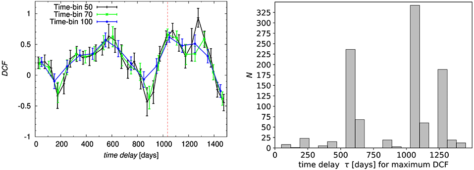
Figure 3. Results of the Discrete Correlation Function (DCF). (Left) DCF as a function of time-delay in the observer frame for three different sizes of the time-bin: 50, 70, and 100 days, see the legend. The largest DCF is consistently at the time-delay of 1,050 days for bigger time-steps of 70–100 days. (Right) Histogram of 1,000 bootstrap runs using random subsample selection. The largest peak is at days.
Finally, several biases and problems of the cross-correlation function which primarily stand out when dealing with sparse and heterogeneous light curves were taken into account in z-transformed DCF (Alexander, 1997). In comparison with the discrete correlation function (Edelson and Krolik, 1988), which bins data pairs into equal time-bins, z-transformed DCF applies equal population binning. It is, therefore, a more suitable and robust method for sparse, irregularly sampled, and heterogeneous pairs of light curves with as few as 12 points per population bin.
We show the calculated zDCF as a function of time delay in the observer frame in Figure 4. The largest zDCF is for the time-delay at τ = 1,050 days (zDCF = 0.76), followed by the smaller peak at τ = 571 days (zDCF = 0.68). We verify the significance of the peak using the maximum likelihood, which also enables us to estimate its uncertainty. We obtain the peak value of τzDCF = days, which is also listed among other methods in Table 1.
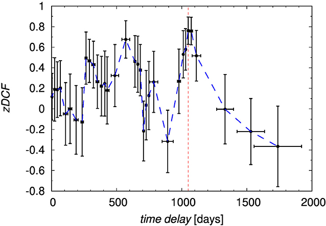
Figure 4. Results of the z-transformed discrete correlation function (zDCF). We show the zDCF as a function of the time-delay in the observer frame. The red vertical dashed line marks the time-delay with the largest value of a zDCF coefficient.
We summarize the time-delay value for CTS C30.10 by calculating the average value for the most prominent peak at ~1,050 days in the observer frame using Table 1. We get the mean value of days in the observer frame, which translates into days in the source frame.
2.2. Radius-Luminosity Relation for MgII
As for Hβ broad line, we construct the radius-luminosity relation for MgII line taking into account our detection of time-lag for MgII in CTS C30.10 as well as the measurements of other sources that also have RM data of MgII: 6 sources from Shen et al. (2016), CTS252 from Lira et al. (2018), and NGC4151 from Metzroth et al. (2006). For an overview of the sources and their characteristics, see Table 3 in Czerny et al. (2019).
In Figure 5, we show the radius-luminosity plot using MgII line time-delay in the rest frame and the monochromatic luminosity at 3,000 Å. We compare the localization of sources with the Bentz RHβ − L5100 relation (Bentz et al., 2013), , where the monochromatic luminosity at 5,100 Å is related to the luminosity at 3,000 Å by an approximate scaling as inferred from the luminosity-dependent bolometric corrections by Netzer (2019). For comparison, we also display the MgII-based radius-luminosity relation as derived by Vestergaard and Osmer (2009): . We see that the majority of the sources follow radius-luminosity relation within uncertainties, with CTS252 being an outlier, which could be the hint of the trend of a smaller time-delay for higher Eddington-ratio sources as was already studied for Hβ measurements (Du et al., 2018; Martínez-Aldama et al., 2019a). Based on the smaller MgII line width, CTS252 is a higher Eddington-ratio source in comparison with CTS C30.10 (Czerny et al., 2019), but the trend needs to be confirmed for a higher number of MgII measurements.
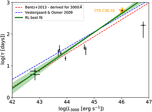
Figure 5. The radius-luminosity relation for MgII broad line using the sources as listed in Table 3 in Czerny et al. (2019) and the new measurement of CTS C30.10 (orange star). The red dashed line stands for the standard Bentz relation RHβ − L5100 (Bentz et al., 2013), derived for 3, 000Å using the bolometric corrections from Netzer (2019): . The blue dashed line is the MgII-based radius-luminosity relation derived by Vestergaard and Osmer (2009): . The green solid line is the best-fit result using the general prescription with K = 1.47 ± 0.06 and α = 0.59 ± 0.06. The shaded region corresponds to 1σ uncertainties.
Excluding CTS252, we fit the radius-luminosity dataset with the general relation . We obtain the best-fit parameters of K = 1.47 ± 0.06 and α = 0.59 ± 0.06. In Figure 5, we see that the best-fit radius-luminosity relation passes nearly through the CTS C30.10 point in comparison with the Bentz relation, which is due to a slightly higher mean slope—α = 0.59 instead of α = 0.53. However, the slopes do not differ within uncertainties and hence the radius-luminosity relation with the expected scaling of R ~ L1/2 so far holds for MgII time-lag measurements.
3. Accretion Rate Effect Over the Radius-Luminosity Relation
The RHβ − L5100 relation offers the possibility of estimate the luminosity distance (DL) independently of the redshift, which is suitable for cosmological applications (Martínez-Aldama et al., 2019a, and references therein). Also, it shows a low scatter (0.13dex, Bentz et al., 2013) and although objects, like NGC5548, show a large variation, the scatter is within uncertainties. However, the recent inclusion of AGN radiating close to the Eddington limit (super-Eddington sources) has increased the scatter significantly. This kind of sources are located on the right-bottom side of the relation (see Figure 1), which implies that the time delay of super-Eddington sources is shorter than the predicted by the RHβ − L5100 relation.
Super-Eddington sources tend to show an extreme behavior respect to the general AGN population: large densities ( cm−3), low-ionization parameters (log U < −2), high intensity of lowest ionization emission lines like FeII and strong outflows in the high-ionization like CIVλ1549 (Marziani et al. 2019 and references therein). These features are probably explained by an optically and geometrically thick slim disk (Wang et al., 2014b), which shields the line emitting region gas from the most intense UV radiation (Marziani et al., 2018). This peculiar behavior is also reflected in the RHβ − L5100 relation by the super-Eddington sources of SEAMBH sample, but also by some objects of SDSS-RM sample. One-third of the SDSS-RM shows an Eddington ratio higher than the average Eddington ratio in Bentz sample, then they also a departure from the expected RHβ − L5100 relation. Therefore, a correction is needed not just for super-Eddington sources, but all sources have to be rescaled.
To estimate this correction to the measured time delay as a function of the accretion rate, we estimate the black hole mass (Equation 1) considering a virial factor anti-correlated with the FWHM of the line recently proposed by Mejía-Restrepo et al. (2018), which in some sense corrects for the orientation effect. For the accretion rate, we will consider the dimensionless accretion rate () introduced by Du et al. (2016). Details of the estimated values are reported in Martínez-Aldama et al. (2019a). To estimate the departure from the RHβ − L5100, we consider the parameter , which is the difference between the time delay observed and estimated from the RHβ − L5100 relation. In the bottom panel of Figure 1 is shown the behavior of ΔRHβ as a function of L5100. Also, in colors, it is shown the variation of the dimensionless accretion rate, where it is clearly observed that largest departures correspond to highest values. The relation between ΔRHβ and can be described by the linear relation:
With this relation, the observed time delay can be corrected by the dimensionless accretion rate effect, decrease the scatter and recover the time delay predicted by the RHβ − L5100 relation. However, this relation is strongly dependent on the virial factor selected for the black hole mass and the accretion rate estimations. The virial factor is still an open problem and although many formalisms have been proposed anyone can be applied to the general AGN population. was modeling with a scarcity of narrow profiles (FWHM <2,000 km s−1), which represent 30% of our full sample. The inclusion of narrow profiles in its modeling could modify the exponent of the anti-correlation and modify our results.
4. Cosmology With Reverberation-Mapped Sources
Recovering the low scatter of the RHβ − L5100 relation after the correction by the dimensionless accretion rate, we were able to build a Hubble diagram (Figure 6) which relates the distance to the sources with the redshift (z) or the velocity recession. The slope of the relation between these two parameters is the value of the Hubble constant (H0), which determines the current expansion rate of the Universe. This parameter has been estimated in the early Universe (z<1,000) using the Cosmic Microwave Background (CMB, Planck Collaboration 2018) and in the late Universe (up to z ~ 1.5) has been using Cepheid stars (Shanks et al. 2019 and references therein) and Supernovae Ia (SNIa, Burns et al. 2018; Macaulay et al. 2019; Riess et al. 2019). The most recent results from the Planck Collaboration (2018) indicate a value of H0 = 67.66 ± 0.42 km s−1 Mpc−1. While the recent ones employing observations of Cepheids stars and SNIa from the Hubble telescope give a value of 74.3 ± 1.42 km s−1 Mpc−1 (Riess et al., 2019). The precision in the determination, <2%, discards the possibility of an error measurement, therefore the disagreement suggests a change in the Hubble constant in the different epochs of the Universe and new physics is required to solve the problem. This problem is called Hubble constant tension. The recent results of Risaliti and Lusso (2019) using quasars at z ~ 4 also show a small gap between the standard ΛCDM model and the fit performed. The large redshift range covered by quasar (0 < z < 7) is suitable for estimating the Hubble constant and addressing the Hubble constant tension.
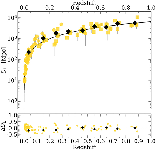
Figure 6. Hubble diagram after the correction by dimensionless accretion rate. Markers and colors are the same as in Figure 1. The black lines indicates the expected luminosity distance based on the standard ΛCDM model. The black diamonds represent the average values for the DL considering redshift bins of Δz = 0.1. The bottom panel shows the difference between the expected luminosity distance and the observed one.
To get the luminosity distance (DL), we estimate L5100 from the Equation (1) and after we use the relation: . In the Figure 6 the black line marks the marks the expected model according to the ΛCDM model. As a visual representation, we show the DL considering redshift bins of Δz = 0.1 (black symbols), which do not have any statistical significance by the number of points. The standard deviation of the errors (0.31, shown in the bottom panel) does not show any particular trend but the dispersion is still large in comparison with other, more matured methods. For the determination of the cosmological constant, we assumed the ΛCDM model and a constant of H0 = 67.66 ± 0.42 km s−1 Mpc−1. Looking for the best fit using a minimization method (χ2), we get the best values for Ωm and ΩΛ. Our results are in agreement with the standard model within 2σ confidence level, however, it is not yet ready to provide new for cosmological constraints, considering that error associated with CMB, Cepheids stars and SNIa are < 2%.
There are still some systematic errors related that have to be corrected. In the previous section, we proposed a correction by the accretion rate effect, but this correction has to be improved since the virial factor has associated large uncertainties. Then, we have to work for clarifying the dynamics of the BLR and the orientation effect. Another important source of error is the method employed in the determination of the time delay. The delay measurements used here are a compilation of the results from the literature, and each group uses different criteria and methods, which also introduces an error when different samples are compared.
In particular, Czerny et al. (2019) and Zajaček et al. (2019) applied six different methods to determine the time-lag between the continuum and MgII line response. These included cross-correlation based techniques ICCF, DCF, zDCF, χ2-based method (Czerny et al., 2013, 2019), the measure of data regularity (von Neumann's estimator; Chelouche et al., 2017), and the JAVELIN code (Just Another Vehicle for Estimating Lags In Nuclei, formerly SPEAR; Zu et al., 2011, 2013, 2016). They showed that for the intermediate-redshift quasar CTS C30.10 (see also section 2.1), the uncertainty in the time-lag determination depends on the approach. If a narrow surrounding of the main peak in time delay measure is taken into consideration, the uncertainty can be of the order of a few days only for the total observing run of 1,000 days and more. The small uncertainty of the order of a few days only was obtained by JAVELIN. On the other hand, if the total range of possible time delays is considered, that is between zero and half of the duration of the observation, the uncertainty can be of the order of 10 and even 100 days depending on the quality of the data. This uncertainty further propagates into the radius-luminosity relation and the Hubble diagram of reverberation mapped quasars. In Figure 7, we illustrate this in terms of constraining cosmological parameters from monitoring of a single source CTS C30.10 mentioned above (dark matter and dark energy fractions) for two different uncertainties—2 days as provided by the JAVELIN code and 22 days that is more representative when other methods are taken into account.
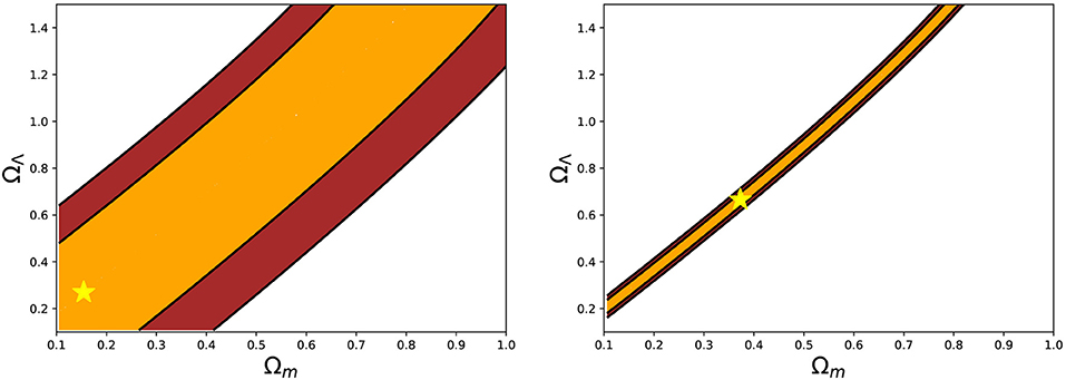
Figure 7. Effect of the time-delay uncertainty on constraining cosmological parameters for the quasar CTS 30.10. The color-coded regions represent the result of χ2 fitting with the star denoting the minimum and the orange and the brown areas stand for 1σ and 2σ uncertainties, respectively. (Left) Time-delay of 562 ± 22 days. (Right) Time-delay of 564 ± 2 days as determined by the JAVELIN code.
Although the error provided by the JAVELIN is underestimated and can be corrected by performing many bootstrap runs to recover the overall time-lag distribution, by combining several robust methods one can achieve the time-lag uncertainty of 5%. Under this assumption, ~625 sources are needed to achieve 2% uncertainty for all cosmological parameters including w0 parameter. However, special attention is needed for the process of a systematic time-lag analysis for the whole sample of reverberation-mapped quasars since currently, the time-lag analysis is largely heterogeneous with different authors using different time-delay methods and their associated uncertainties. This is a source of large systematic uncertainties that will need to be addressed in future RM samples of quasars.
Quasars are complex objects and many corrections are still needed to consider these objects like standard candles suitable for cosmology. However, Cepheids star and SNIa have been also corrected for the shape of the lightcurve, extinction and the host galaxy, and sophisticated observational methods have been proposed for getting better observations (e.g., Scolnic et al., 2018). All this effort is reflected in the low uncertainties associated with the cosmological results. A similar situation should be happening with quasars taking advantage of their broad range of redshift and luminosity.
5. Photometric Reverberation Mapping in the LSST Era
5.1. AGN Science With LSST
LSST will be a public optical/NIR survey of ~half the sky in the ugrizy bands upto r ~27.5 based on ~820 visits across all the six photometric bands over a 10-years period (Ivezić et al., 2019). The 8.4 m telescope with a state-of-the-art 3.2 Gigapixel flat-focal array camera will allow performing rapid scans of the sky with 15 s exposure and thus providing a moving array of color images of objects that change. The whole observable sky is planned to be scanned every ~4 nights. It is expected that upon the completion of the main-survey period, LSST will have mapped ~20 billion galaxies and ~ 17 billion stars using these six photometric bands4.
The LSST AGN survey will produce a high-purity sample of at least 10 million well-defined, optically-selected AGNs (see section 5.2). Utilizing the large sky coverage, depth, the six filters extending to 1 μm, and the valuable temporal information of LSST, this AGN survey will supersede the largest current AGN samples by more than an order of magnitude. Each region of the LSST sky will receive ~200 visits in each band in the decade long monitoring, allowing variability to be explored on timescales from minutes to a decade [see Chapter 10 of LSST Science Collaboration et al. (2009) for more details]. LSST will conduct more intense observations of at least 4 Deep Drilling Fields or DDFs, i.e., COSMOS, XMM-LSS, W-CDF-S, and ELAIS-S1, each of which cover ~10 deg2 (more details in Brandt et al. 2018). Brandt et al. (2018) estimates an increase in the depth in the DDFs by over an order of magnitude relative to the main-survey. This will be made possible owing to a ~18–20X increase in the number of visits per photometric band.
LSST will be assisted by an array of campaigns (Brandt and Vito, 2017) during its proposed run. Moreover, there is a need for follow-up spectroscopic campaigns, i.e., SDSS-V Black Hole Mapper (Kollmeier et al., 2017), which aim to derive BLR properties and reliable SMBH masses for distant AGNs with expected observed-frame reverberation lags of 10–1,000 days. The SDSS-V Black Hole Mapper survey will also perform reverberation mapping campaigns in three out of the four LSST DDFs. LSST will provide additional high quality photometry for these sources that will substantially improve these estimations. The proposed cadence (~2 nights) of the observations of AGNs and the expected re-visits during the 10-years run will allow to (1) ensure a high lag recovery fraction for the relatively short accretion-disk lags expected (Yu et al., 2018); and (2) allow investigations of secular evolution of these lags that test the underlying model. LSST will also perform quality accretion disk reverberation mapping for ~3,000 AGNs in the DDFs.
5.2. Suitability of Quasar Monitoring
Every night, LSST will monitor ~75 million AGNs and is estimated to detect ~300+ million AGNs in the ~18,000 deg2 main-survey area (Luo et al., 2017). Taking into account factors like obscuration and host-galaxy contamination that will hinder this AGN selection, optimistic estimates predict around ~20 million (from LSST alone) and ~50+ million (LSST+ others) AGNs to be reliably monitored.
5.2.1. Type-1 Quasar Counts
In the context of the reverberation mapping, one intends to focus on the broad emission lines that are a characteristics of Type-1 AGNs (Netzer and Peterson, 1997; Peterson et al., 2004; Gravity Collaboration et al., 2018). With LSST, we would want to constrain the quasar counts in terms of only Type 1 AGNs with respect to the observed broad emission lines, such as Hβ, MgII, CIV. We perform a simple filtering to estimate these numbers in terms of total predicted number of quasars to be observed over the full duration of LSST.
Three entities affect our estimation of the “good” Type 1 quasars, namely (1) the line intensity; (2) overlap of the photometric bands; and (3) the line FWHM. The peak intensity of the line (including continuum) that will be acquired from the pipeline, is already convolved with the filters and to recover the true intensity one needs to scale by , where T is the throughput (or transmittance) of the corresponding band which is estimated from the band function. We adopt a throughput value of 0.2 to exclude the gaps between the consecutive bands (see Figure 8). To get an idea of the impact of the line FWHM on the quasar number counts, we adopted the mean values for the broad emission lines—Hβ, MgII, from the SDSS DR7 Quasar catalog (Shen et al., 2011). The average values for the FWHM are: 4,662.26 ± 2,181.53kms−1 (MgII) and 4,903.63 ± 3,119.26kms−1 (Hβ). For simplicity, we adopt the values 4,500 km s−1 (MgII) and 5,000 km s−1 (Hβ) for this preliminary analysis. Since, the emission lines in consideration are “broad,” we estimate the equivalent width of MgII and Hβ to account for the broadness in these line profiles. We estimate this additional width from the mean FWHMs and the values obtained are ~42 Å and ~80 Å for MgII and Hβ, respectively. Next, we retrieve the wavelength windows where these photometric bands overlap (see Table 2). As we have assumed the throughput value of 0.2, we exclude the u-band since the peak transmittance in this band is ~0.14. This is the reason why the first entry in Table 2 is in the g-band (for MgII; rest-frame wavelength = 2,799.12Å) and the wavelength is recovered corresponds to the intersection with the throughput value, T = 0.2 on the lower wavelength side of the band. In the case for Hβ, the starting value z = 0 is inclusive (rest-frame wavelength for Hβ = 4,861.36Å). The remaining entries in Table 2 are identical. We estimate that ~26% (for MgII) and ~36% (for Hβ) of the supposed Type 1 quasars will end up being observed in these overlapping windows taking into account the respective emission lines broadening and our naive assumption of the throughput cutoff. Figure 9 shows an illustrative view of this analysis in a more general context.
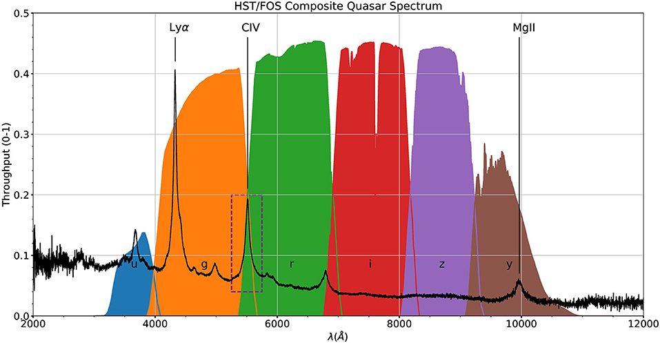
Figure 8. Throughput curves for the 6 LSST photometric bands (ugrizy), shown as a function of wavelength (in Å). The black solid line is the HST/FOS composite quasar spectrum (Zheng et al., 1997) and the dashed box in purple highlights the importance of quasar selection. The spectrum is shown at a redshift, z = 2.56. The composite spectrum is downloaded from https://archive.stsci.edu/prepds/composite_quasar/.
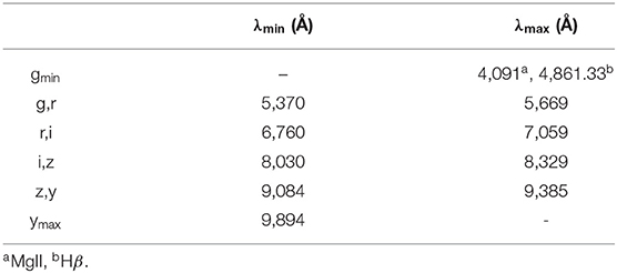
Table 2. LSST photometric bands: overlapping windows.
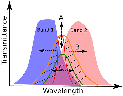
Figure 9. A representative illustration for the quasar selection based on distribution of (A) line intensities; (B) band overlaps, and (C) line widths. Three instances of emission line profiles are shown in orange, red, and green, and the patched region highlights the importance of the broad distribution of equivalent widths (EWs) in quasars. The arrows mark the direction of the effect due to these three factors.
The expected number of Type 2 quasars is estimated to be ~50–70% of the total population (Schmitt et al., 2001; Hao et al., 2005; Elitzur, 2012). So, if we start with a total population, for example, 1 million, we will have about 300,000–500,000 Type 1 AGNs based on this filtering. Next, the actual fraction of the “good” quasars will be ~22–37% (MgII) and ~19–32% (Hβ) after applying our filter due to the band overlap. It is expected that the filter wheel to be installed on LSST will have five slots (the filter wheel will prioritize griz and the y and u filters will be alternated for the fifth slot) complementary to the SDSS filter design (Fukugita et al., 1996). This means that at any given time, the image will be taken with one of the filters in-line with the camera. The filter replacement takes about 2 min to complete and this filter replacement will be performed 2–6 times per night and the total number of filter changes through the survey is 14,194 (LSST Science Collaboration et al., 2017). The remaining filter will be substituted for one of the existing filters in the filter-wheel (most likely u-band in place of y-band). This will affect the quasar counts based on the quality of the data, where quality is directly related to the number of re-visits for the source.
5.3. Modeling “Real” Light Curves
LSST is a photometric project but the 6-channel photometry (see Figure 8) can be effectively used for the purpose of reverberation mapping and estimation of time delays. We present some preliminary results from our software in development which allows to produce mock light curves and recover the time delays. The code takes into consideration several key parameters to produce these light curves, namely—(1) the campaign duration of the instrument (10 years); (2) number of visits per photometric band; (3) the photometric accuracy (0.01–0.1 mag)5; (4) black hole mass distribution6; (5) luminosity distribution7; (6) redshift distribution8; and (7) line equivalent widths (EWs) consistent with SDSS quasar catalog (Shen et al., 2011). We create continuum stochastic lightcurve for a quasar of an assumed magnitude and redshift from AGN power spectrum with Timmer-Koenig algorithm (Timmer and Koenig, 1995). The code takes as an input a first estimate for the time delay measurement. We utilize the standard RHβ − L5100 relation (Bentz et al., 2013) to estimate this value. In the current version of the code, the results for the photometric reverberation method are estimated by adopting only two photometric channels at a time and the time delay is estimated using the χ2 method. We account for the contamination in the emission line (Hβ, MgII, CIV) as well as the in the continuum. The code also incorporates the FeII pseudo-continuum and contamination from starlight, i.e., stellar contribution.
In Martínez-Aldama et al. (2019b), we show preliminary results from our code. In that paper, we show the variation in the simulated lightcurves for MgII and Hβ as a function of the redshift and luminosity and their corresponding time-delay distributions. The power spectral distribution for these lightcurves was assumed to have the low-frequency break corresponding to 2,000 days. In Figure 10, we show the results from subsequent analysis performed using two-channel setup. We incorporate a higher density of the continuum and the line contribution owing to the fact that in the DDFs the probing will be denser compared to the rest of the All-Sky survey. The computations are performed for a representative case of black hole mass, . The photometric accuracy is kept at 0.01 and the low-frequency break corresponds to between 200 and 300 days. The EWs are increased by a factor of 3 with respect to the average values (MgII: 47 Å and Hβ: 87 Å) which were used in the previous results. The corresponding time-delays (with dispersion) recovered from the analyses are reported for the respective emission line (MgII and Hβ) and two representative cases of the luminosity, erg s−1 and 1046erg s−1. The dispersions for the reported time-delays are found to be within ~1–2% limit.
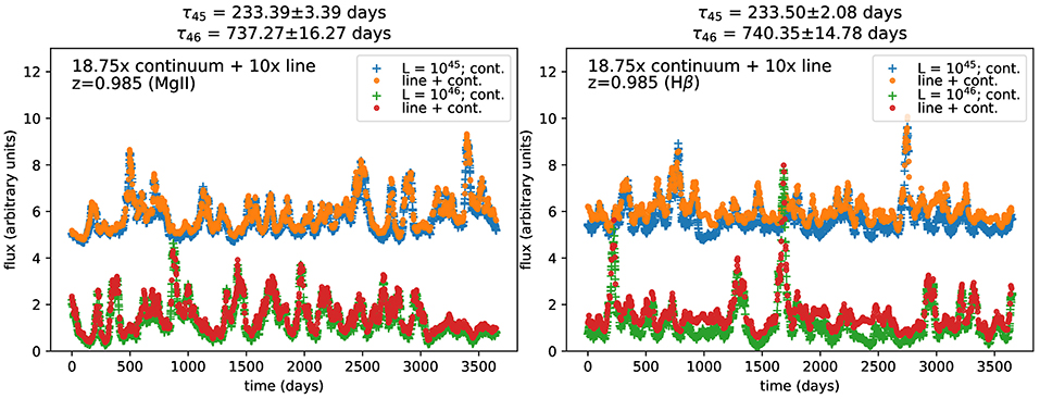
Figure 10. Simulated lightcurves for Mg II and Hβ at z = 0.985. The lightcurves are generated using Timmer-Koenig method (Timmer and Koenig, 1995) and combining with photometric data from LSST (Ivezić et al., 2019). Two cases of luminosity (1045 and 1046 erg s−1) are shown, each for the continuum and the line. The continuum and the line contributions are made denser by a factor of 18.75 and 10, respectively. The lightcurves with luminosity 1045 erg s−1 is shifted by factor of 4.5 with respect to the lightcurves with luminosity 1046 erg s−1 to highlight the differences between the two cases. The corresponding time delays are reported on top of each plot for these two cases of luminosity. The simulations are currently performed using two channels.
6. Discussions
The MgII and Hβ both are low-Ionization broad-emission lines, however, MgII shows a narrower profile than Hβ profile (Marziani et al., 2013), suggesting that the emission line is emitted in an outer region. In Śniegowska et al. (2018), we have tested that their emissivity profiles using CLOUDY reveals similar emitting zones in the BLR. When compared to their corresponding FeII emission, the maximum MgII and Hβ emission peaks are ~107 cm deeper from the face of the BLR cloud. Yet, these emitting zones are extended, spanning across ~6 orders in cloud depth. There have been recent studies that predict that the most efficient MgII emitting clouds are always near the outer physical boundary of the BLR, while the Balmer line gas is inside this outer BLR boundary (Guo et al., 2019). This explains the low variability shown by MgII in comparison to Hβ. Since MgII usually does not display a “breathing mode,” it suggests that there is not a Radius-Luminosity relation for this line. However, the possibility of a global Radius-Luminosity is viable, as long as the outer radius of the BLR scales with the black hole mass (Guo et al., 2019). The Radius-Luminosity relation for MgII (Figure 5) shows a slope of α = 0.59 ± 0.06, which is in agreement with the idea of a general R-L relation.
As has been shown in this paper, the Eddington ratio plays an important role in the RHβ − L5100. This is straightforward as we see that if the line width is fixed but we recover a lower time delay than expected and subsequently the black hole mass estimated is lower. Hence, the Eddington ratio that we estimate will be higher. This trend of decrease of the time delay with rising Eddington ratio seems systematic (Grier et al., 2017; Martínez-Aldama et al., 2019a). Being able to constrain their physical parameter space (in terms of the ionization parameter, cloud density and accretion rate) and link this to the observables, such as emission line ratios and shape of the emission line profiles, would provide answers to this anomaly (Panda et al. in prep).
The next steps in the code development for modeling the light curves, include testing with different methodologies to generate lightcurves, e.g., Damped-Random Walk. This also applies to the time-delay estimation where we are testing the consistency of the predicted values with other available methods, e.g., Interpolated cross-correlation function (Gaskell and Peterson, 1987) and JAVELIN (Zu et al., 2011, 2013, 2016). In the near future, we plan to extend the analysis taking into account contribution from all the 6 channels, including the lag between the images when going from one filter to the next and including the filter replacement time as explained in section 5.2.1. Finally, we plan to create lightcurves incorporating a distribution of the redshift, luminosity, MBH and EWs.
A special attention should be paid to realistic estimates of the uncertainties of different time-lag methods (ICCF, DCF, zDCF, JAVELIN, χ2, regularity measures-von Neumann estimator, see Zajaček et al., 2019, for a general overview and the comparison) since this is one of the main sources of the scatter of the radius-luminosity relation. The effect of systematic errors on the time-lag uncertainty was analyzed by Yu et al. (2019), who compared JAVELIN and ICCF methods using simulated light curves, with JAVELIN performing better in terms of uncertainty determination. A similar result is reached by Li et al. (2019) who compare ICCF, JAVELIN, and zDCF methods using generated light curves that mock multi-object spectroscopic reverberation mapping (MOS-RM) surveys. They conclude that JAVELIN and ICCF outperform zDCF, with JAVELIN generally introducing the lowest bias into the radius-luminosity relation. However, more comparison and analysis is needed using both the observed reverberation-mapped quasars (e.g., bootstrap algorithm) as well as simulated light curves (generated by both Timmer-Koenig algorithm and damped random walk for comparison) for the traditional (ICCF, DCF, zDCF) and other, novel methods of the time-lag determination (von Neumann, χ2 methods), with the special focus on how time-delay uncertainties propagate into constraining cosmological parameters (Czerny et al., 2013).
7. Conclusions
Reverberation mapping studies have been quite successful to constrain the RBLR − Lλ relation for various broad emission lines (Hβ: Grier et al. 2017 and references therein; MgII: Metzroth et al. 2006; Czerny et al. 2013; Lira et al. 2018; Czerny et al. 2019; CIV: Grier et al. 2019 and references therein). In this contribution, we present the monitoring of the intermediate-redshift quasar CTS C30.10 by the SALT telescope over the course of 6 years and detected the time-delay of MgII-line response of τMgII = days in the source frame. In combination with other sources where MgII time-delay was detected, we constructed the radius-luminosity relation considering a sample of 117 sources taken from the literature, and fitted it with the general power-law relation , with the best-fit coefficients of K = 1.47 ± 0.06 and α = 0.59 ± 0.06, which are within uncertainties consistent with the values of RHβ − L5100 relation by Bentz et al. (2013). It is thus possible to use the radius-luminosity relation also toward higher redshifts using MgII and potentially CIV line. Under the assumption that the time-delay can be measured within 5% uncertainty, about 625 sources are needed in future surveys to constrain the cosmological parameters with 2% uncertainty.
Along RHβ − L5100 relation there is an effect of the accretion rate, which induces a departure from the expected value, i.,e., super-Eddington sources show a time delay shorter than the expected. This effect can be corrected, recovering the classical low scatter in the relation. With the estimation of the luminosity distance, we estimated the cosmological parameters. The results are in agreement with the ΛCDM model within 2σ confidence level, which is still not suitable for cosmological results. Unfortunately, there are still some systematic errors that have to be corrected. The current sample size for such studies has now reached ≳100 and future reverberation campaigns promise to increase this sample by manifolds and get accurate cosmological results. Also, an improvement in the method for the determination of the time delay and a better understanding of the AGN properties (e.g., inclination angle) are required to decrease the errors and get better results (Panda et al., 2019).
LSST is one of the forerunners in such future campaigns which will cover a wide range of wavelength (3,050 Å ≲ λ ≲ 11,000 Å) and this instrument alone will provide ~5 orders increase in the number of reverberation-mapped quasars. With LSST we will have no dearth in the number of quasars, yet if we are to find answers to some of the long-standing questions in astronomy with the help of quasars, we would require to improve the quality of the observed data from the instrument. In this paper, we provide the foundation for a filtering algorithm that will be useful for the community to account for the “good” quasars especially for the purpose of variability studies and photometric reverberation mapping. The suitability of these good quasars is based on three fundamental criteria—the emission line intensity, the band overlap and the line width. We also show the first results from our code designed to create synthetic, stochastic lightcurves incorporating fundamental quasar properties and the instrument's performance as per Ivezić et al. (2019). This will be useful—first for preparing a mock catalog of quasar lightcurves, and second, to test real data that will be obtained from the LSST in the near future.
Data Availability Statement
All datasets generated for this study are included in the article/supplementary material.
Author Contributions
SP has contributed toward the section 5. MLM-A has contributed toward the sections 3 and 4. MZ has contributed toward the section 2. The Introduction, Discussions, and Conclusions have been jointly prepared by all the authors.
Funding
The project was partially supported by National Science Centre, Poland, grant No. 2017/26/A/ST9/00756 (Maestro 9), and by the MNiSW grant DIR/WK/2018/12.
Conflict of Interest
The authors declare that the research was conducted in the absence of any commercial or financial relationships that could be construed as a potential conflict of interest.
Acknowledgments
We cordially thank all the organizers of Symposium 2 Quasars in cosmology organized at EWASS 2019 in Lyon on June 25–26, 2019, in particular Bożena Czerny, Paola Marziani, Edi Bon, Natasha Bon, Elisabeta Lusso, and Mauro D'Onofrio.
Footnotes
1. ^For more details see https://www.lsst.org/.
2. ^Where FWHM is the full width at half-maximum of the corresponding emission line profile.
3. ^The use of the double Lorentzian profiles is motivated from the study for this source in Modzelewska et al. (2014). The value of the χ2 obtained for the double Lorentzian is the lowest (see their Table 3).
4. ^See Ivezić et al. (2019) for a complete review on LSST science drivers, telescope design and data products.
5. ^These values are adopted from Ivezić et al. (2019).
6. ^The results shown here are for a representative black hole mass, MBH = 108 M⊙.
7. ^The results shown here are for two representative cases of bolometric luminosity, Lbol = 1045 and 1046 erg s−1.
8. ^The results shown here are for two representative cases of redshifts, z = 0.1 and 0.985.
References
LSST Science Collaboration, Abell, P. A., Allison, J., Anderson, S. F., Andrew, J. R., Angel, J. R. P., et al. (2009). LSST science book, version 2.0. arXiv [Preprint]. arXiv:0912.0201. Available online at: https://ui.adsabs.harvard.edu/abs/2009arXiv0912.0201L/abstract
Alexander, T. (1997). Is AGN variability correlated with other AGN properties? ZDCF analysis of small samples of sparse light curves, in Astronomical Time Series, Volume 218 of Astrophysics and Space Science Library, eds Maoz, D., Sternberg, A., and Leibowitz, E. M., (Tel-Aviv: Springer), 163.
Barth, A. J., Pancoast, A., Bennert, V. N., Brewer, B. J., Canalizo, G., Filippenko, et al. (2013). The lick AGN monitoring project 2011: Fe II reverberation from the outer broad-line region. Astrophys. J. 769:128. doi: 10.1088/0004-637X/769/2/128
Bentz, M. C., Cackett, E. M., Crenshaw, D. M., Horne, K., Street, R., and Ou-Yang, B. (2016). A reverberation-based black hole mass for MCG-06-30-15. Astrophys. J. 830:136. doi: 10.3847/0004-637X/830/2/136
Bentz, M. C., Denney, K. D., Grier, C. J., Barth, A. J., Peterson, B. M., Vestergaard, M., et al. (2013). The low-luminosity end of the radius-luminosity relationship for active galactic nuclei. Astrophys. J. 767:149. doi: 10.1088/0004-637X/767/2/149
Bentz, M. C., Horenstein, D., Bazhaw, C., Manne-Nicholas, E. R., Ou-Yang, B. J., Anderson, M., et al. (2014). The mass of the central black hole in the nearby Seyfert galaxy NGC 5273. Astrophys. J. 796:8. doi: 10.1088/0004-637X/796/1/8
Bentz, M. C., Peterson, B. M., Netzer, H., Pogge, R. W., and Vestergaard, M. (2009). The radius-luminosity relationship for active galactic nuclei: the effect of host-galaxy starlight on luminosity measurements. II. The full sample of reverberation-mapped AGNs. Astrophys. J. 697, 160–181. doi: 10.1088/0004-637X/697/1/160
Bentz, M. C., Peterson, B. M., Pogge, R. W., Vestergaard, M., and Onken, C. A. (2006). The radius-luminosity relationship for active galactic nuclei: the effect of host-galaxy starlight on luminosity measurements. Astrophys. J. 644, 133–142. doi: 10.1086/503537
Blandford, R. D., and McKee, C. F. (1982). Reverberation mapping of the emission line regions of Seyfert galaxies and quasars. Astrophys. J. 255, 419–439.
Brandt, W. N., Ni, Q., Yang, G., Anderson, S. F., Assef, R. J., Barth, A. J., et al. (2018). Active galaxy science in the LSST deep-drilling fields: footprints, cadence requirements, and total-depth requirements. arXiv [Preprint]. arXiv:1811.06542. Available online at: https://ui.adsabs.harvard.edu/abs/2018arXiv181106542B/abstract
Brandt, W. N., and Vito, F. (2017). High-redshift active galactic nuclei and the next decade of Chandra and XMM-Newton. Astron. Nachr. 338, 241–248. doi: 10.1002/asna.201713337
Burns, C. R., Parent, E., Phillips, M. M., Stritzinger, M., Krisciunas, K., Suntzeff, N. B., et al. (2018). The Carnegie Supernova project: absolute calibration and the Hubble constant. Astrophys. J. 869:56. doi: 10.3847/1538-4357/aae51c
Chelouche, D., Pozo-Nuñez, F., and Zucker, S. (2017). Methods of reverberation mapping. I. Time-lag determination by measures of randomness. Astrophys. J. 844:146. doi: 10.3847/1538-4357/aa7b86
Collier, S., Horne, K., Wanders, I., and Peterson, B. M. (1999). A new direct method for measuring the Hubble constant from reverberating accretion discs in active galaxies. Monthly Notices R. Astron. Soc. 302, L24–L28.
Collin, S., Kawaguchi, T., Peterson, B. M., and Vestergaard, M. (2006). Systematic effects in measurement of black hole masses by emission-line reverberation of active galactic nuclei: Eddington ratio and inclination. Astron. Astrophys. 456, 75–90. doi: 10.1051/0004-6361:20064878
Collin-Souffrin, S., Dyson, J. E., McDowell, J. C., and Perry, J. J. (1988). The environment of active galactic nuclei. I–A two-component broad emission line model. Monthly Notices R. Astron. Soc. 232, 539–550.
Czerny, B., and Hryniewicz, K. (2011). The origin of the broad line region in active galactic nuclei. Astron. Astrophys. 525:L8. doi: 10.1051/0004-6361/201016025
Czerny, B., Hryniewicz, K., Maity, I., Schwarzenberg-Czerny, A., Życki, P. T., and Bilicki, M. (2013). Towards equation of state of dark energy from quasar monitoring: Reverberation strategy. Astron. Astrophys. 556:A97. doi: 10.1051/0004-6361/201220832
Czerny, B., Li, Y.-R., Hryniewicz, K., Panda, S., Wildy, C., Sniegowska, M., et al. (2017). Failed radiatively accelerated dusty outflow model of the broad line region in active galactic nuclei. I. Analytical solution. Astrophys. J. 846:154. doi: 10.3847/1538-4357/aa8810
Czerny, B., Olejak, A., Rałowski, M., Kozłowski, S., Loli Martinez Aldama, M., Zajacek, M., et al. (2019). Time delay measurement of Mg II line in CTS C30.10 with SALT. Astrophys. J. 880:46. doi: 10.3847/1538-4357/ab2913
Du, P., Hu, C., Lu, K.-X., Huang, Y.-K., Cheng, C., Qiu, J., et al. (2015). Supermassive black holes with high accretion rates in active galactic nuclei. IV. Hβ time lags and implications for super-Eddington accretion. Astrophys. J. 806:22. doi: 10.1088/0004-637X/806/1/22
Du, P., Lu, K.-X., Zhang, Z.-X., Huang, Y.-K., Wang, K., Hu, C., et al. (2016). Supermassive black holes with high accretion rates in active galactic nuclei. V. A new size-luminosity scaling relation for the broad-line region. Astrophys. J. 825:126. doi: 10.3847/0004-637X/825/2/126
Du, P., Zhang, Z.-X., Wang, K., Huang, Y.-K., Zhang, Y., Lu, K.-X., et al. (2018). Supermassive black holes with high accretion rates in active galactic nuclei. IX. 10 New observations of reverberation mapping and shortened Hβ lags. Astrophys. J. 856:6. doi: 10.3847/1538-4357/aaae6b
Edelson, R. A., and Krolik, J. H. (1988). The discrete correlation function—a new method for analyzing unevenly sampled variability data. Astrophys. J. 333, 646–659.
Elitzur, M. (2012). On the unification of active galactic nuclei. Astrophys. J. 747:L33. doi: 10.1088/2041-8205/747/2/L33
Elvis, M., and Karovska, M. (2002). Quasar parallax: a method for determining direct geometrical distances to Quasars. Astrophys. J. Lett. 581, L67–L70. doi: 10.1086/346015
Fausnaugh, M. M., Grier, C. J., Bentz, M. C., Denney, K. D., De Rosa, G., Peterson, B. M., et al. (2017). Reverberation mapping of optical emission lines in five active galaxies. Astrophys. J. 840:97. doi: 10.3847/1538-4357/aa6d52
Fukugita, M., Ichikawa, T., Gunn, J. E., Doi, M., Shimasaku, K., and Schneider, D. P. (1996). The Sloan digital sky survey photometric system. Astron. J. 111:1748.
Gaskell, C. M. (2009). What broad emission lines tell us about how active galactic nuclei work. New Astron. Rev. 53, 140–148. doi: 10.1016/j.newar.2009.09.006
Gaskell, C. M., and Peterson, B. M. (1987). The accuracy of cross-correlation estimates of quasar emission-line region sizes. Astrophys. J Suppl. Ser. 65, 1–11.
Gravity Collaboration, Abuter, R., Accardo, M., Amorim, A., Anugu, N., Ávila, G., et al. (2017). First light for GRAVITY: phase referencing optical interferometry for the very large telescope interferometer. Astron. Astrophys. 602:A94. doi: 10.1051/0004-6361/201730838
Gravity Collaboration, Sturm, E., Dexter, J., Pfuhl, O., Stock, M. R., Davies, R. I., et al. (2018). Spatially resolved rotation of the broad-line region of a quasar at sub-parsec scale. Nature 563, 657–660. doi: 10.1038/s41586-018-0731-9
Grier, C. J., Shen, Y., Horne, K., Brandt, W. N., Trump, J. R., Hall, P. B., et al. (2019). The Sloan digital sky survey reverberation mapping project: initial CIV lag results from four years of data. arXiv [Preprint]. arXiv:1904.03199. Available online at: https://ui.adsabs.harvard.edu/abs/2019arXiv190403199G/abstract
Grier, C. J., Trump, J. R., Shen, Y., Horne, K., Kinemuchi, K., McGreer, I. D., et al. (2017). The Sloan digital sky survey reverberation mapping project: Hα and Hβ reverberation measurements from first-year spectroscopy and photometry. Astrophys. J. 851:21. doi: 10.3847/1538-4357/aa98dc
Guo, H., Shen, Y., He, Z., Wang, T., Liu, X., Wang, S., et al. (2019). Understanding broad Mg II variability in Quasars with photoionization. arXiv [Preprint]. arXiv:1907.06669. Available online at: https://ui.adsabs.harvard.edu/abs/2019arXiv190706669G/abstract
Haas, M., Chini, R., Ramolla, M., Pozo Nuñez, F., Westhues, C., Watermann, R., et al. (2011). Photometric AGN reverberation mapping–an efficient tool for BLR sizes, black hole masses, and host-subtracted AGN luminosities. Astron. Astrophys. 535:A73. doi: 10.1051/0004-6361/201117325
Hao, L., Strauss, M. A., Tremonti, C. A., Schlegel, D. J., Heckman, T. M., Kauffmann, G., et al. (2005). Active galactic nuclei in the Sloan digital sky survey. I. Sample selection. Astrophys. J. 129, 1783–1794. doi: 10.1086/428485
Horne, K., Korista, K. T., and Goad, M. R. (2003). Quasar tomography: unification of echo mapping and photoionization models. Monthly Notices R. Astron. Soc. 339, 367–386. doi: 10.1046/j.1365-8711.2003.06036.x
Hu, C., Du, P., Lu, K.-X., Li, Y.-R., Wang, F., Qiu, J., et al. (2015). Supermassive black holes with high accretion rates in active galactic nuclei. III. Detection of Fe II reverberation in nine narrow-line Seyfert 1 galaxies. Astrophys. J. 804:138. doi: 10.1088/0004-637X/804/2/138
Ivezić, Ž., Kahn, S. M., Tyson, J. A., Abel, B., Acosta, E., Allsman, R., et al. (2019). LSST: from science drivers to reference design and anticipated data products. Astrophys. J. 873:111. doi: 10.3847/1538-4357/ab042c
Kaspi, S., Maoz, D., Netzer, H., Peterson, B. M., Vestergaard, M., and Jannuzi, B. T. (2005). The relationship between luminosity and broad-line region size in active galactic nuclei. Astrophys. J. 629, 61–71. doi: 10.1086/431275
Kaspi, S., Smith, P. S., Netzer, H., Maoz, D., Jannuzi, B. T., and Giveon, U. (2000). Reverberation measurements for 17 Quasars and the size-mass-luminosity relations in active galactic nuclei. Astrophys. J. 533, 631–649. doi: 10.1086/308704
Kollmeier, J. A., Zasowski, G., Rix, H.-W., Johns, M., Anderson, S. F., Drory, N., et al. (2017). SDSS-V: pioneering panoptic spectroscopy. arXiv [Preprint]. arXiv:1711.03234. Available online at: https://ui.adsabs.harvard.edu/abs/2017arXiv171103234K/abstract
Laor, A., Jannuzi, B. T., Green, R. F., and Boroson, T. A. (1997). The ultraviolet properties of the narrow-line Quasar I Zw 1. Astrophys. J. 489, 656–671.
Li, J. I.-H., Shen, Y., Brandt, W. N., Grier, C. J., Hall, P. B., et al. (2019). The Sloan digital Sky Survey Reverberation Mapping Project: comparison of lag measurement methods with simulated observations. Astrophys. J. 884, 119. doi: 10.3847/1538-4357/ab41fb
Lira, P., Kaspi, S., Netzer, H., Botti, I., Morrell, N., Mejía-Restrepo, J., et al. (2018). Reverberation mapping of luminous Quasars at high z. Astrophys. J. 865:56. doi: 10.3847/1538-4357/aada45
LSST Science Collaboration, Marshall, P., Anguita, T., Bianco, F. B., Bellm, E. C., Brandt, N., et al. (2017). Science-driven optimization of the LSST observing strategy. arXiv [Preprint]. arXiv:1708.04058. Available online at: https://ui.adsabs.harvard.edu/abs/2017arXiv170804058L/abstract
Lu, K.-X., Du, P., Hu, C., Li, Y.-R., Zhang, Z.-X., Wang, K., et al. (2016). Reverberation mapping of the broad-line region in NGC 5548: evidence for radiation pressure? Astrophys. J. 827:118. doi: 10.3847/0004-637X/827/2/118
Luo, B., Brandt, W. N., Xue, Y. Q., Lehmer, B., Alexander, D. M., Bauer, F. E., et al. (2017). The Chandra deep field-south survey: 7 Ms source catalogs. Astrophys. J. Suppl. Ser. 228:2. doi: 10.3847/1538-4365/228/1/2
Macaulay, E., Nichol, R. C., Bacon, D., Brout, D., Davis, T. M., Zhang, B., et al. (2019). First cosmological results using type Ia supernovae from the dark energy survey: measurement of the Hubble constant. Monthly Notices R. Astron. Soc. 486, 2184–2196. doi: 10.1093/mnras/stz978
Martínez-Aldama, M. L., Czerny, B., Kawka, D., Karas, V., Panda, S., Zajaček, M., et al. (2019a). Can reverberation-measured quasars be used for cosmology? Astrophys. J. 883, 170. doi: 10.3847/1538-4357/ab3728
Martínez-Aldama, M. L., Panda, S., Czerny, B., and Zajaček, M. (2019b). Quasars from LSST as dark energy tracers: first steps. arXiv [Preprint]. arXiv:1910.02725. Available online at: https://ui.adsabs.harvard.edu/abs/2019arXiv191002725L/abstract
Marziani, P., del Olmo, A., Martínez-Carballo, M. A., Martínez-Aldama, M. L., Stirpe, G. M., Negrete, C. A., et al. (2019). Black hole mass estimates in quasars. A comparative analysis of high- and low-ionization lines. Astron. Astrophys. 627:A88. doi: 10.1051/0004-6361/201935265
Marziani, P., Dultzin, D., Sulentic, J. W., Del Olmo, A., Negrete, C. A., Martínez-Aldama, M. L., et al. (2018). A main sequence for quasars. Front. Astron. Space Sci. 5:6. doi: 10.3389/fspas.2018.00006
Marziani, P., Sulentic, J. W., Plauchu-Frayn, I., and del Olmo, A. (2013). Is MgIIλ2800 a reliable virial broadening estimator for quasars? Astron. Astrophys. 555:A89. doi: 10.1051/0004-6361/201321374
Maza, J., Ruiz, M. T., Gonzalez, L. E., Wischnjewsky, M., and Antezana, R. (1993). Calan-Tololo Survey. V. Two hundred new southern quasars. Rev. Mex. Astron. Astrofís. 25, 51–57.
McLure, R. J., and Jarvis, M. J. (2002). Measuring the black hole masses of high-redshift quasars. Monthly Notices R. Astron. Soc. 337, 109–116. doi: 10.1046/j.1365-8711.2002.05871.x
Mejía-Restrepo, J. E., Lira, P., Netzer, H., Trakhtenbrot, B., and Capellupo, D. M. (2018). The effect of nuclear gas distribution on the mass determination of supermassive black holes. Nat. Astron. 2, 63–68. doi: 10.1038/s41550-017-0305-z
Metzroth, K. G., Onken, C. A., and Peterson, B. M. (2006). The mass of the central black hole in the Seyfert galaxy NGC 4151. Astrophys. J. 647, 901–909. doi: 10.1086/505525
Modzelewska, J., Czerny, B., Hryniewicz, K., Bilicki, M., Krupa, M., Świȩtoń, A., et al. (2014). SALT long-slit spectroscopy of CTS C30.10: two-component Mg II line. Astron. Astrophys. 570:A53. doi: 10.1051/0004-6361/201424332
Netzer, H. (2013). The Physics and Evolution of Active Galactic Nuclei. New York, NY: Cambridge University Press.
Netzer, H. (2019). Bolometric correction factors for active galactic nuclei. Monthly Notices R. Astron. Soc. 488, 5185–5191. doi: 10.1093/mnras/stz2016
Netzer, H., and Peterson, B. M. (1997). Reverberation mapping and the physics of active galactic nuclei, in Astronomical Time Series, Volume 218 of Astrophysics and Space Science Library, eds Maoz, D., Sternberg, A., and Leibowitz, E. M., (Tel-Aviv: Springer), 85.
Panda, S., Marziani, P., and Czerny, B. (2019). The Quasar main sequence explained by the combination of Eddington ratio, metallicity, and orientation. Astrophys. J. 882:79. doi: 10.3847/1538-4357/ab3292
Pei, L., Barth, A. J., Aldering, G. S., Briley, M. M., Carroll, C. J., Carson, D. J., et al. (2014). Reverberation mapping of the KEPLER field AGN KA1858+4850. Astrophys. J. 795:38. doi: 10.1088/0004-637X/795/1/38
Peterson, B. M., Ferrarese, L., Gilbert, K. M., Kaspi, S., Malkan, M. A., Maoz, D., et al. (2004). Central masses and broad-line region sizes of active galactic nuclei. II. A homogeneous analysis of a large reverberation-mapping database. Astrophys. J. 613, 682–699. doi: 10.1086/423269
Peterson, B. M., Wanders, I., Horne, K., Collier, S., Alexander, T., Kaspi, S., et al. (1998). On uncertainties in cross-correlation lags and the reality of wavelength-dependent continuum lags in active galactic nuclei. Publ. Astron. Soc. Pac. 110, 660–670.
Planck Collaboration, Aghanim, N., Akrami, Y., Ashdown, M., Aumont, J., Baccigalupi, C., et al. (2018). Planck 2018 results. VI. Cosmological parameters. arXiv [Preprint]. arXiv:1807.06209. Available online at: https://ui.adsabs.harvard.edu/abs/2018arXiv180706209P/abstract
Riess, A. G., Casertano, S., Yuan, W., Macri, L. M., and Scolnic, D. (2019). Large Magellanic cloud cepheid standards provide a 1% foundation for the determination of the Hubble constant and stronger evidence for physics beyond ΛCDM. Astrophys. J. 876:85. doi: 10.3847/1538-4357/ab1422
Risaliti, G., and Lusso, E. (2019). Cosmological constraints from the Hubble diagram of Quasars at high redshifts. Nat. Astron. 3, 272–277. doi: 10.1038/s41550-018-0657-z
Robertson, D. R. S., Gallo, L. C., Zoghbi, A., and Fabian, A. C. (2015). Searching for correlations in simultaneous X-ray and UV emission in the narrow-line Seyfert 1 galaxy 1H 0707-495. Monthly Notices R. Astron. Soc. 453, 3455–3460. doi: 10.1093/mnras/stv1575
Schmitt, H. R., Antonucci, R. R. J., Ulvestad, J. S., Kinney, A. L., Clarke, C. J., and Pringle, J. E. (2001). Testing the unified model with an infrared-selected sample of Seyfert galaxies. Astrophys. J. 555, 663–672. doi: 10.1086/321505
Scolnic, D. M., Jones, D. O., Rest, A., Pan, Y. C., Chornock, R., Foley, R. J., et al. (2018). The complete light-curve sample of spectroscopically confirmed SNe Ia from pan-STARRS1 and cosmological constraints from the combined pantheon sample. Astrophys. J. 859:101. doi: 10.3847/1538-4357/aab9bb
Shanks, T., Hogarth, L. M., and Metcalfe, N. (2019). Gaia cepheid parallaxes and ‘local hole’ relieve H0 tension. Monthly Notices R. Astron. Soc. 484, L64–L68. doi: 10.1093/mnrasl/sly239
Shapovalova, A. I., Popović, L. Č., Burenkov, A. N., Chavushyan, V. H., Ilić, D., Kovačević, A., et al. (2012). Spectral optical monitoring of the narrow-line Seyfert 1 galaxy Ark 564. Astrophys. J. Suppl. Ser. 202:10. doi: 10.1088/0067-0049/202/1/10
Shen, Y., Horne, K., Grier, C. J., Peterson, B. M., Denney, K. D., Trump, J. R., et al. (2016). The Sloan digital sky survey reverberation mapping project: first broad-line Hβ and Mg II Lags at z ≳ 0.3 from six-month spectroscopy. Astrophys. J. 818:30. doi: 10.3847/0004-637X/818/1/30
Shen, Y., Richards, G. T., Strauss, M. A., Hall, P. B., Schneider, D. P., Snedden, S., et al. (2011). A catalog of Quasar properties from Sloan digital sky survey data release 7. Astrophys. J. Suppl. Ser. 194:45. doi: 10.1088/0067-0049/194/2/45
Śniegowska, M., Kozłowski, S., Czerny, B., and Panda, S. (2018). Quasar main sequence in the UV plane. arXiv [Preprint]. arXiv:1810.09363. Available online at: https://ui.adsabs.harvard.edu/abs/2018arXiv181009363S/abstract
Sulentic, J., Marziani, P., and Zamfir, S. (2011). The case for two Quasar populations. Balt. Astron. 20, 427–434. doi: 10.1515/astro-2017-0314
Sulentic, J. W., Bachev, R., Marziani, P., Negrete, C. A., and Dultzin, D. (2007). C IV λ1549 as an eigenvector 1 parameter for active galactic nuclei. Astrophys. J. 666, 757–777. doi: 10.1086/519916
Sulentic, J. W., Marziani, P., Zamanov, R., Bachev, R., Calvani, M., and Dultzin-Hacyan, D. (2002). Average Quasar spectra in the context of eigenvector 1. Astrophys. J. Lett. 566, L71–L75. doi: 10.1086/339594
Sulentic, J. W., Marziani, P., and Zamfir, S. (2009). Comparing H β line profiles in the 4D eigenvector 1 context. New Astron. Rev. 53, 198–201. doi: 10.1016/j.newar.2009.06.001
Sun, M., Grier, C. J., and Peterson, B. M. (2018). PyCCF: Python Cross Correlation Function for reverberation mapping studies. ascl:1805.032. Available online at: https://ui.adsabs.harvard.edu/abs/2018ascl.soft05032S
Véron-Cetty, M. P., Véron, P., and Gonçalves, A. C. (2001). A spectrophotometric atlas of narrow-Line Seyfert 1 galaxies. Astron. Astrophys. 372, 730–754. doi: 10.1051/0004-6361:20010489
Vestergaard, M., and Osmer, P. S. (2009). Mass functions of the active black holes in distant Quasars from the large bright Quasar survey, the Bright Quasar survey, and the color-selected sample of the SDSS fall equatorial stripe. Astrophys. J. 699, 800–816. doi: 10.1088/0004-637X/699/1/800
Vestergaard, M., and Peterson, B. M. (2006). Determining central black hole masses in distant active galaxies and Quasars. II. Improved optical and UV scaling relationships. Astrophys. J. 641, 689–709. doi: 10.1086/500572
Wandel, A., Peterson, B. M., and Malkan, M. A. (1999). Central masses and broad-line region sizes of active galactic nuclei. I. Comparing the photoionization and reverberation techniques. Astrophys. J. 526, 579–591.
Wang, J.-M., Du, P., Hu, C., Netzer, H., Bai, J.-M., Lu, K.-X., et al. (2014a). Supermassive black holes with high accretion rates in active galactic nuclei. II. The most luminous standard candles in the universe. Astrophys. J. 793:108. doi: 10.1088/0004-637X/793/2/108
Wang, J.-M., Qiu, J., Du, P., and Ho, L. C. (2014b). Self-shadowing effects of slim accretion disks in active galactic nuclei: the diverse appearance of the broad-line region. Astrophys. J. 797:65. doi: 10.1088/0004-637X/797/1/65
Watson, D., Denney, K. D., Vestergaard, M., and Davis, T. M. (2011). A new cosmological distance measure using active galactic nuclei. Astrophys. J. Lett. 740:L49. doi: 10.1088/2041-8205/740/2/L49
Woo, J.-H., Yoon, Y., Park, S., Park, D., and Kim, S. C. (2015). The black hole mass-stellar velocity dispersion relation of narrow-line Seyfert 1 galaxies. Astrophys. J. 801:38. doi: 10.1088/0004-637X/801/1/38
Yu, Z., Kochanek, C. S., Peterson, B. M., Zu, Y., Brandt, W. N., Cackett, E. M., et al. (2019). On reverberation mapping lag uncertainties. arXiv [Preprint]. arXiv:1909.03072. Available online at: https://ui.adsabs.harvard.edu/abs/2019arXiv190903072Y/abstract
Yu, Z., Martini, P., Davis, T. M., Gruendl, R. A., Hoormann, J. K., Kochanek, C. S., et al. (2018). Quasar accretion disk sizes from continuum reverberation mapping in the DES standard star fields. arXiv [Preprint]. arXiv:1811.03638. Available online at: https://ui.adsabs.harvard.edu/abs/2018arXiv181103638Y/abstract
Zajaček, M., Czerny, B., Martínez-Aldama, M. L., and Karas, V. (2019). Reverberation mapping of distant quasars: Time lag determination using different methods. Astron. Nachr. 340, 577–585. doi: 10.1002/asna.201913659
Zamfir, S., Sulentic, J. W., Marziani, P., and Dultzin, D. (2010). Detailed characterization of Hβ emission line profile in low-z SDSS quasars. Monthly Notices R. Astron. Soc. 403, 1759–1786. doi: 10.1111/j.1365-2966.2009.16236.x
Zhang, Z.-X., Du, P., Smith, P. S., Zhao, Y., Hu, C., Xiao, M., et al. (2019). Kinematics of the Broad-line Region of 3C 273 from a 10 yr Reverberation Mapping Campaign. Astrophys. J. 876, 49. doi: 10.3847/1538-4357/ab1099
Zheng, W., Kriss, G. A., Telfer, R. C., Grimes, J. P., and Davidsen, A. F. (1997). A composite HST spectrum of Quasars. Astrophys. J. 475, 469–478.
Zu, Y., Kochanek, C. S., Kozłowski, S., and Peterson, B. M. (2016). Application of stochastic modeling to analysis of photometric reverberation mapping data. Astrophys. J. 819:122. doi: 10.3847/0004-637X/819/2/122
Zu, Y., Kochanek, C. S., Kozłowski, S., and Udalski, A. (2013). Is Quasar optical variability a damped random walk? Astrophys. J. 765:106. doi: 10.1088/0004-637X/765/2/106
Keywords: quasars: reverberation mapping, time-delay measurements, cosmology, instrument: LSST, photometry, spectroscopy
Citation: Panda S, Martínez-Aldama ML and Zajaček M (2019) Current and Future Applications of Reverberation-Mapped Quasars in Cosmology. Front. Astron. Space Sci. 6:75. doi: 10.3389/fspas.2019.00075
Received: 13 September 2019; Accepted: 27 November 2019;
Published: 11 December 2019.
Edited by:
Paola Marziani, Osservatorio Astronomico di Padova (INAF), ItalyReviewed by:
Alenka Negrete, National Autonomous University of Mexico, MexicoGiovanna Maria Stirpe, Osservatorio di Astrofisica e Scienza dello Spazio di Bologna (INAF), Italy
Copyright © 2019 Panda, Martínez-Aldama and Zajaček. This is an open-access article distributed under the terms of the Creative Commons Attribution License (CC BY). The use, distribution or reproduction in other forums is permitted, provided the original author(s) and the copyright owner(s) are credited and that the original publication in this journal is cited, in accordance with accepted academic practice. No use, distribution or reproduction is permitted which does not comply with these terms.
*Correspondence: Swayamtrupta Panda, cGFuZGFAY2Z0LmVkdS5wbA==