Magnetic Field Turbulence in the Solar Wind at Sub‐ion Scales: In Situ Observations and Numerical Simulations

We investigate the transition of the solar wind turbulent cascade from MHD to sub‐ion range by means of a detailed comparison between in situ observations and hybrid numerical simulations. In particular, we focus on the properties of the magnetic field and its component anisotropy in Cluster measurements and hybrid 2D simulations. First, we address the angular distribution of wave vector in the kinetic range between ion and electron scales by studying the variance anisotropy of the magnetic field components. When taking into account a single-direction sampling, like that performed by spacecraft in the solar wind, the main properties of the fluctuations observed in situ are also recovered in our numerical description. This result confirms that solar wind turbulence in the sub‐ion range is characterized by a quasi-2D gyrotropic distribution of k-vectors around the mean field. We then consider the magnetic compressibility associated with the turbulent cascade and its evolution from large-MHD to sub‐ion scales. The ratio of field aligned to perpendicular fluctuations, typically low in the MHD inertial range, increases significantly when crossing ion scales and its value in the sub‐ion range is a function of the total plasma beta only, as expected from theoretical predictions, with higher magnetic compressibility for higher beta. Moreover, we observe that this increase has a gradual trend from low to high beta values in the in situ data; this behavior is well captured by the numerical simulations. The level of magnetic field compressibility that is observed in situ and in the simulations is in fairly good agreement with theoretical predictions, especially at high beta, suggesting that, in the kinetic range explored, the turbulence is supported by low-frequency and highly oblique fluctuations in pressure balance, like kinetic Alfvén waves or other slowly evolving coherent structures. The resulting scaling properties as a function of the plasma beta and the main differences between numerical and theoretical expectations and in situ observations are also discussed.

1. Introduction

The solar wind constitutes a unique laboratory for plasma turbulence (Bruno and Carbone, 2013). In the last decade, increasing interest has been raised toward the small-scale behavior of the turbulent cascade, i.e., beyond the breakdown of the fluid/MHD description that takes place at ion scales. Spacecraft observations of solar wind and near-Earth plasmas provide unique measurements of the turbulent fluctuations at scales comparable and smaller than the typical particle scales, the Larmor radius ρ (see Appendix for definition of physical quantities used), and the inertial length d (e.g., Alexandrova et al., 2009; Sahraoui et al., 2010; Alexandrova et al., 2012; Chen et al., 2013a). However, the physical processes governing the energy cascade at kinetic scales and those responsible for its final dissipation are not well understood yet.

What is well established is that, in the transition from MHD to the kinetic regime, plasma turbulence modifies its characteristics. Observational and numerical studies over the last few years have highlighted the main differences between large and small-scale properties of solar wind fluctuations (e.g., Chen, 2016; Cerri et al., 2019). The magnetic field spectrum typically steepens when approaching ion scales, leading at sub‐ion scales (between ion and electron typical scales) to a power law with spectral index close to $-2.8$ (Alexandrova et al., 2009, 2012; Kiyani et al., 2009; Chen et al., 2010; Sahraoui et al., 2013), steeper than Kolmogorov −5/3 but also than the theoretical prediction $-7/3$ from EMHD (Biskamp et al., 1996) and (kinetic Alfvén waves) KAW/whistler turbulence (Schekochihin et al., 2009; Boldyrev et al., 2013). The origin of such a spectral slope is still unknown and it has been proposed that it could be related to intermittency corrections (Boldyrev and Perez, 2012; Landi et al., 2019), magnetic reconnection (Loureiro and Boldyrev, 2017; Mallet et al., 2017; Cerri et al., 2018), Landau damping (Howes et al., 2008; Schreiner and Saur, 2017), and the role of the nonlinearity parameter (Passot and Sulem, 2015; Sulem et al., 2016).

The change in the magnetic field spectrum is accompanied by a rapid decrease in the power of ion velocity fluctuations (Šafránková et al., 2013; Stawarz et al., 2016) and the onset of the nonideal terms in Ohm’s law which governs the electric field associated with the turbulent fluctuations (Stawarz et al., 2020); as a consequence, the electric field spectrum becomes shallower at sub‐ion scales (Franci et al., 2015a; Matteini et al., 2017). In this framework, the electric current (mostly carried by electrons) plays a major role, coupling directly with the magnetic field in the cascade and likely affecting the energy cascade rate via the Hall term (Hellinger et al., 2018; Papini et al., 2019; Bandyopadhyay et al., 2020). All these properties depend further on the plasma beta ($\beta =8\pi n{k}_{B}T/B^2$), which controls, among other things, the scale at which the magnetic field spectrum breaks (Chen et al., 2014; Franci et al., 2016; Wang et al., 2018; Woodham et al., 2018).

One of the most significant differences with respect to the turbulent regime observed at large scales however is the role of compressive effects. While in the inertial range fluctuations show a low level of both plasma and magnetic field compressibility and hence can be reasonably well described by incompressible MHD, at sub‐ion scales density and magnetic field intensity fluctuations become significant and comparable to transverse ones (Alexandrova et al., 2008; Sahraoui et al., 2010; Chen et al., 2012b; Salem et al., 2012; Kiyani et al., 2013; Perrone et al., 2017), in agreement with simulations (Franci et al., 2015b; Parashar et al., 2016; Cerri et al., 2017). It is believed that this is related to a change in the properties of the turbulent fluctuations, which become intrinsically compressive at small scales. It is then by studying in detail their properties that it is possible to shed light on the nature of the fluctuations which support the cascade at kinetic scales (Chen et al., 2013b; Grošelj et al., 2019; Pitňa et al., 2019; Alexandrova et al., 2020).

Another important aspect of solar wind turbulence is its spectral anisotropy (Horbury et al., 2008; Chen et al., 2010; Wicks et al., 2010; Roberts et al., 2017b). Studies about the shape of turbulent eddies, both at MHD (Chen et al., 2012a; Verdini et al., 2018, 2019) and at kinetic scales (Wang et al., 2020), reveal the presence of a 3D anisotropy in the structures when described in terms of a local frame. On the other hand, when the analysis is made in a global frame (without tracking the local orientation of the structures), the 3D anisotropy is not captured, and the k-vectors of the fluctuations show a statistical quasi-2D distribution around the magnetic field (Matthaeus et al., 1990; Dasso et al., 2005; Osman and Horbury, 2006). In this work, we address this latter aspect and we investigate the distribution of the k-vectors with respect to the ambient magnetic field at kinetic scales by using the magnetic field variance anisotropy (i.e., the ratio of magnetic field fluctuations in different components). Bieber et al. (1996) and Saur and Bieber (1999) have shown that, also in single spacecraft observations, it is possible to characterize the 3D k-vector distribution by using variance anisotropy. When the sampling occurs only along a preferential direction, like in typical solar wind observations, their model predicts various possible kinds of variance anisotropy as a function of the underlying k-spectrum. In particular, assuming a quasi-2D gyrotropic distribution of k-vectors (axisymmetric with respect to the magnetic field), the ratio of the power in the two perpendicular magnetic field components is directly related to the local slope of the spectrum, which is assumed to have the same form for all components and a slope independent of the scale within a given regime. Since both quantities, spectral slope and perpendicular power ratio, can be easily measured in situ, the Saur and Bieber model constitutes a useful and simple tool to investigate underlying spectral anisotropies. Despite the model was originally developed for MHD scale fluctuations, it basically corresponds to a geometrical description built on the divergence-less condition for $\mathit{B}$, so it can be applied to any kind of regimes, including the low-frequency turbulence expected at sub‐ion scales (Turner et al., 2011). In the work of Lacombe et al. (2017), we investigated the k-vector distribution at sub‐ion scales using the technique by Saur and Bieber (1999). Based on the comparison with the predictions, we concluded that the distribution of the k-vectors in the sub‐ion range of solar wind turbulence is consistent with a quasi-2D gyrotropic spectrum, then approaching a more isotropic shape when reaching electron scales (Lacombe et al., 2017). However, such an application has not been benchmarked by kinetic numerical studies yet.

The aim of this work is then to focus on the spectral anisotropy properties and magnetic compressibility at small scales, by exploiting the detailed comparison of in situ observations and high-resolution kinetic numerical simulations. The paper is organized as follows: In Section 2, we introduce the spacecraft and numerical dataset used, and in Section 3, we describe their spectral properties. In Section 4, we discuss the spectral anisotropy at sub‐ion scales and test, for the first time, the Saur and Bieber model in numerical kinetic simulations; in Section 5, we address properties of the magnetic compressibility and its dependence on the plasma beta. Finally, in Section 6, we discuss our conclusions and the implications of our findings for the interpretation of solar wind observations and simulations.

2. Data and Simulations

In this study, we compare the properties of magnetic fluctuations measured in situ by the Cluster spacecraft with numerical results obtained by means of 2D hybrid particle-in-cell (PIC) simulations.

2.1. Cluster STAFF Spectra

For our analysis, we use the dataset discussed by Alexandrova et al. (2012), when Cluster was in the free solar wind, i.e., not magnetically connected to the Earth’s bow shock. Details have been described also in Lacombe et al. (2017) and we recall here the main aspects. Magnetic field fluctuations are measured by the STAFF (Spatiotemporal Analysis of Field Fluctuation) instrument, composed of a waveform unit (SC) and a Spectral Analyzer (SA). Power spectra are computed on board in a magnetic field-aligned system of coordinates (MFA), based on the 4 s magnetic field measured by the FGM (Fluxgate Magnetometer) experiment. A selection of 112 spectra has been performed, retaining in each spectrum only measurements above three times the noise level in every direction $x,y$, and z (see Appendix in Lacombe et al., 2017). Each sample is a 10 min average of 150 individual 4 s spectral measurements. This provides spectra above 1 Hz up to typically 20–100 Hz, depending on the amplitude of the fluctuations in each interval. When converted into physical length scales, assuming the Taylor hypothesis ($k=2\pi f/V_{sw}$), this leads to signals that cover the range between $\sim 2d_p$ and $\sim 0.5d_e$ (where $d_p$ and $d_e$ are the proton and electron inertial lengths, respectively), enabling then a good description of the sub‐ion regime from proton to electron scales.

The reference frame adopted (MFA) is such that $B_z$ is the component aligned with the mean magnetic field $B_0$ (relative to the 4 s interval during which an individual spectrum is calculated); $B_x$ is the component orthogonal to $B_z$ in the plane containing both the solar wind velocity $V_{sw}$ and the mean magnetic field $B_0$; and $B_y$ is the third orthogonal component. Note that a selection criterium is imposed on the angle ${\theta }_{BV}$, the angle between the local 4 s magnetic field, and the flow velocity; i.e., that ${\theta }_{BV}$ is large enough to avoid a connection with the Earth bow shock during the sampled interval; ${\theta }_{BV}$ in the dataset has an average value of $\sim 80$°. This implies that, for each spectrum, the mean magnetic field makes a big angle with respect to the sampling direction; moreover, we have checked that ${\theta }_{BV}$ does not vary significantly during the 10 min over which spectra are averaged.

As a consequence, this procedure selects intervals in which Cluster observed highly oblique k-vectors and, to a good approximation, the component $B_x$ corresponds also to the sampling direction (radial) and is orthogonal to $B_0$; $B_y$ corresponds to the other perpendicular component; and $B_z$ is identified as the compressive component $B_{\parallel }$. As already discussed in Lacombe et al. (2017), although the total trace power measured in situ is an invariant observable, the fact that the sampling occurs only in a preferred direction introduces a relative weight between $B_x$ and $B_y$ that is measurement dependent (Saur and Bieber, 1999). To take this into account, we have employed an analogous approach in the analysis of the simulations data, as described in the next section.

2.2. Hybrid 2D Numerical Simulations

In situ observations are directly compared with numerical simulations performed with the hybrid-PIC code CAMELIA (Matthews, 1994; Franci et al., 2018a). Despite the fact that the hybrid model neglects the dynamics of electrons, it captures well the transition from fluid to kinetic regime around ion scales where electron effects do not play an important role. Hybrid simulations reproduce successfully many of the main properties of solar wind turbulence observed by spacecraft at sub‐ion scales (e.g., Perrone et al., 2013; Valentini et al., 2014; Franci et al., 2015a; Franci et al., 2015b; Franci et al., 2018b; Cerri et al., 2016; Cerri et al., 2017; Arzamasskiy et al., 2019). It is then a suitable tool to investigate the turbulent regime probed by STAFF/Cluster data. We use here 2D simulations—computationally more affordable than 3D—in order to explore the parameter space observed in situ; in particular, we focus on the effects associated with variations in the proton and electron plasma beta ${\beta }_p$ and ${\beta }_e$. The restricted 2D geometry clearly cannot fully capture the richness of the turbulent phenomena (e.g., Howes, 2015) and in general, kinetic aspects related to the propagation of the fluctuations along the magnetic field are inhibited, like the presence of parallel propagating ion-scale waves and associated cyclotron resonances or the development of some kinetic instabilities (although some of their aspects can be still described also in 2D, e.g., Hellinger et al., 2015; Hellinger et al., 2017). On the other hand, in the case of the highly anisotropic solar wind turbulence, spectral properties can be captured efficiently (Franci et al., 2015a; Franci et al., 2015b). In particular, for the purpose of this work, Franci et al. (2016) have shown that 2D hybrid simulations are able to reproduce the ion-break scale behavior in different beta regimes observed in solar wind turbulence (Chen et al., 2014). Moreover, 3D hybrid simulations (Franci et al., 2018b) have confirmed the solidity of the reduced 2D results and the good agreement with in situ observations. We then exploit the good matching between simulations and in situ observations to characterize further the properties of kinetic plasma turbulence in the sub‐ion regime.

In order to make a direct comparison with sub‐ion spectra measured by Cluster, we have adopted a similar approach in the computation of spectra in the simulations. This means that numerical spectra are computed along the x direction only, to mimic the radial sampling occurring in the solar wind. This is obtained by integrating along y the Fourier spectrum $P\left(k_x,y\right)$ of each i magnetic field component:

$P_i\left(k_x\right)={{\displaystyle \int }}^{\text{}}{P}_i\left(k_x,y\right)dy.(1)$

Therefore, also in the simulation, $B_x$ corresponds to the sampling direction, orthogonal to the out-of-plane magnetic field $B_z$, and $B_y$ is the most energetic fluctuating component, being orthogonal to both $B_0$ and $k=k_x$. With this approach and within the observational conditions previously described, we can perform a direct comparison of simulations and in situ data.

The numerical dataset used was originally presented in Franci et al. (2016) and is available online. It is constituted by a set of different ${2048}^2$ 2D simulations of decaying turbulence, corresponding to a physical simulation box size of ${256}^2{d}_i$, except for the higher beta case, ${\beta }_p=8$, where the size is ${512}^2{d}_i$, and for different beta conditions covering the range of variations observed in situ, with ${\beta }_p={\beta }_e$. Runs are initiated with random perpendicular Alfvénic fluctuations with vanishing cross-helicity and equipartition in magnetic and kinetic energies. The rms of the in-plane fluctuations is $B^{rms}=0.24B_0$ and the highest initially excited k-vector is $k^{inj}{d}_i=0.2$ ($B^{rms}=0.48B_0$ and $k^{inj}{d}_i=0.05$ for the ${\beta }_p=8$ case). Spectra are computed at the maximum of the turbulent activity.

3. In Situ Data Analysis and Simulation Results

Figure 1 shows three examples of Cluster spectra (2003/02/18 04:45–04:55; 2004/02/22 05:40–05:50; 2004/01/22 04:40–04:50), where frequencies have been converted into k-vectors and normalized to $d_p$ (original sampling frequencies are also shown for reference). Observations cover ion and electron scales, with a transition accompanied by a slope change around $k{d}_p\sim 10$. In this work, we focus on the sub‐ion regime highlighted in yellow in the panels, where electron physics effects can be neglected (at least for spectral properties) and a well-defined slope close to $-2.8$ can be observed (Alexandrova et al., 2012). The three cases, corresponding to different total beta β regimes $[0.8,1.5,4]$, show a similar qualitative behavior: as expected, the spectrum $P_y$ of the perpendicular $B_y$ component (blue) is always the most energetic. The power in the other perpendicular component $P_x$ (black dashed) is always slightly smaller; however, its ratio with $P_y$ is roughly independent of beta and close to the local spectral slope (bottom panels); this is related to the 3D distribution of k-vectors (Lacombe et al., 2017) and will be discussed more in detail in Section 4.

FIGURE 1

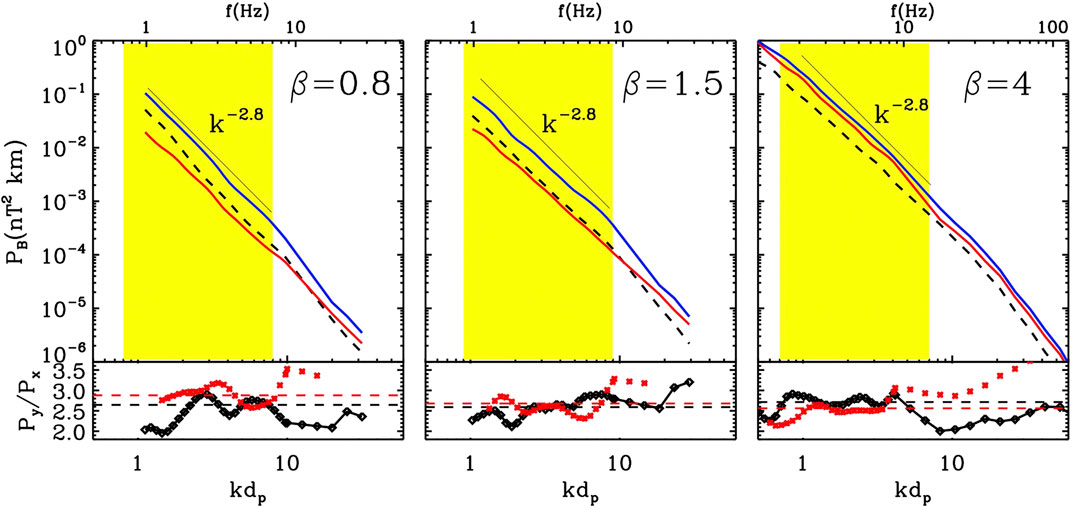
FIGURE 1. Cluster STAFF spectra for different intervals with $\beta =0.8,1.5,4$ from left to right. Colors encode the magnetic field components $B_x$ (black dashed), $B_y$ (blue), and $B_z$ (red). The region highlighted in yellow corresponds to the sub‐ion range investigated in this study. Bottom panels show the ratio of the power in the perpendicular components $P_y\left(k\right)/P_x\left(k\right)$ (black diamonds) and the value γ of the local slope of the total spectrum $P\left(k\right)\sim k^{-\gamma }$ (red stars). The average values of $P_y\left(k\right)/P_x\left(k\right)$ and γ in the sub‐ion range are also shown as horizontal dashed lines.

On the other hand, the power $P_z$ of the field-aligned component $B_z$ (red) is typically less energetic than $P_y$; however, its relative contribution is highly variable with beta: $P_z$ is smaller than $P_x$ for $\beta <1$, comparable to $P_x$ for $\beta \sim 1$, and larger the $P_x$ for $\beta >1$. This obviously results in variable magnetic compressibility associated with the fluctuations and its functional dependence on beta is the subject of Section 5.

Figure 2 shows an analogous selection from numerical simulations; note that, in the simulations, ${\beta }_e={\beta }_p$. In this case, the regime reproduced in the simulation box includes the MHD inertial range and its transition to a sub‐ion cascade at smaller scales. The yellow area highlights the region of the spectra—roughly a decade between $k{d}_p\sim 1$ and $k{d}_p\sim 10$—that can be directly compared with the in situ data. In this region, the qualitative behavior of the spectra is similar to Figure 1: $B_y$ (blu) is always dominant, $B_x$ (black) contributes for a constant fraction of it and is roughly the same at all betas, while $B_z$ (red) varies significantly in the panels and becomes comparable to $B_y$ for large betas. This confirms that our method of computing spectra in the simulations mimicking satellite observations really captures the main aspects of in situ measurements and can then be exploited to investigate further the properties of the turbulent cascade.

FIGURE 2

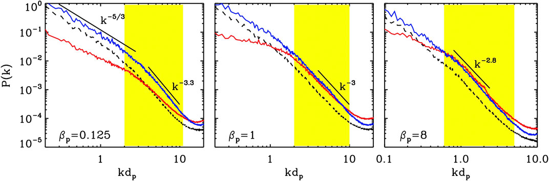
FIGURE 2. Magnetic field spectra from hybrid simulations for different beta regimes (${\beta }_p=0.125,\mathrm{1,10}$ and ${\beta }_e={\beta }_p$). Components are encoded as in Figure 1 and the colored region indicates the sub‐ion range that can be directly compared with the analogous region in the observations.

4. Spectral Anisotropy

4.1. Perpendicular Components Ratio

Bieber et al. (1996) and Saur and Bieber (1999) have investigated how different types of k-vectors distributions can generate a variable anisotropy in the observed magnetic field components, due to sampling effects. In the case of a gyrotropic 2D distribution of k-vectors, the ratio $P_y/P_x$ is expected to coincide with the local slope γ of the spectrum $P\left(k\right)\sim k^{-\gamma }$. This applies well to solar wind observations in the physical range of interest here, as it can be appreciated in Figure 1, where the ratio $P_y/P_x$, shown in the bottom panels, is close to the spectral slope observed—typically in the range [−2.5,−3]—and appears roughly independent of the plasma beta. Interestingly, at smaller scales, when the magnetic spectrum steepens as approaching electron scales (Alexandrova et al., 2009), this is not associated with an increase in the perpendicular power ratio $P_y/P_x$ (which on the contrary has a slight decrease); this does not correspond to the expectation for a quasi-2D spectrum according to the model and in fact, Lacombe et al. (2017) have interpreted this signature as the result of a more isotropic distribution of k-vectors close to electron scales.

To validate further this observational conclusion, we verify here the applicability of the Saur and Bieber model to sub‐ion scale turbulence. In the simulations, the spectrum is two-dimensional by construction and consistent with the axisymmetric initial conditions imposed in the x-y plane, it is also gyrotropic with respect to the out-of-plane magnetic field $B_z$.

First, it is instructive to discuss spectra shown in Figure 3. These are power spectra of the perpendicular components $B_x$ (purple) and $B_y$ (orange) as a function of $k_x$, assuming then a fixed direction of sampling. As expected, $P_y\left(k_x\right)>P_x\left(k_x\right)$; on the other hand, their sum $P_{\perp }\left(k_x\right)$ (solid black line) is statistically equivalent to the axisymmetric spectrum $P_{\perp }\left(k\right)=P_y\left(k\right)+P_x\left(k\right)$. The difference is that when calculating the axisymmetric spectrum $P_{\perp }\left(k\right)$, all perpendicular magnetic field directions have equal weight and one can assume that statistically $P_y\left(k\right)\sim P_x\left(k\right)$; as a consequence, the power associated with any individual perpendicular component corresponds to half of the total perpendicular power $P_{\perp }\left(k\right)/2\sim P_{\perp }\left(k_x\right)/2$ (thin dashed black line). It is interesting to note that when sampling along a fixed direction (x), as it happens with spacecraft in the solar wind, none of the two measured spectra $P_y\left(k_x\right)$ and $P_x\left(k_x\right)$ is really representative of the power $P_{\perp }\left(k\right)/2$ of the gyrotropic description; instead, the component along the sampling ($B_x$) is significantly reduced due to the solenoidal $\nabla \cdot \mathbf{B}=0$ condition, while the orthogonal ($B_y$) is amplified, in order to maintain the same total power $P_{\perp }\left(k\right)$. This means that, in solar wind spectra like in Figure 1, neither $P_x$ nor $P_y$ is individually representative of the average power in a perpendicular B component: the individual measurements of $P_x$ or $P_y$ cannot be directly associated with it, but only their sum.

FIGURE 3

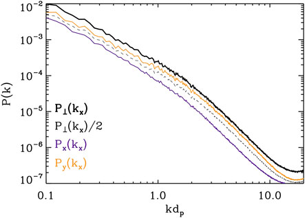
FIGURE 3. Reduced spectra of the fluctuations of the magnetic field components $B_y$ and $B_x$ defined with respect to a fixed sampling direction $k_x$ for a simulation with ${\beta }_p=0.5$. The thick solid black line corresponds to the total perpendicular power $P_{\perp }\left(k_x\right)$; the dashed line shows $P_{\perp }\left(k_x\right)/2$, also corresponding to the average power in any perpendicular magnetic field component in the axisymmetric case.

Bearing this in mind, Figure 4 shows the ratio of the power in the perpendicular components for the three simulations shown in Figure 2. The $P_y/P_x$ ratio captures well the transition from MHD to a steeper spectrum at smaller scales; in all cases, the ratio, close to 5/3 at large scales, starts increasing in the vicinity of ion scales and reaches a maximum in the sub‐ion regime, where it is saturated close to $\sim 3$, in good agreement with the local spectral slope observed in the kinetic range, which is typically close to $-3$. At larger k, the ratio then decreases due to the noise. In the framework of the spectral anisotropy, Saur and Bieber model all this indicates a quasi-2D gyrotropic spectrum of the fluctuations, which corresponds well to the spectrum developed in these simulations. This confirms that the model is valid also at sub‐ion scales and reinforces the finding of Lacombe et al. (2017), where is found that solar wind spectra at kinetic scales are described well by a quasi-2D gyrotropic distribution.

FIGURE 4

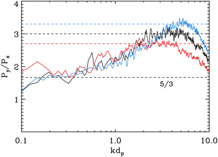
FIGURE 4. Hybrid simulations: spectra of the ratio of the perpendicular magnetic components $P_y\left(k_x\right)/P_x\left(k_x\right)$ and corresponding to the local spectral slope. Different colors encode different ${\beta }_p$: 0.125 (cyan), 1 (black), and 8 (red). The horizontal dashed lines show reference spectral slopes observed in the simulations at $k{d}_p<1$ (−5/3) and at sub‐ion scales $k{d}_p>1$.

4.2. Beta Dependence

There is another interesting indication suggested by Figure 4, namely, the fact that the $P_y/P_x$ ratio in the sub‐ion range seems to depend on beta: consistent with this, the sub‐ion slope in Figure 2 is slightly steeper for small ${\beta }_p$ and shallower for larger ${\beta }_p$. This behavior is already discussed in Franci et al. (2016) and is found in all simulations for the spectrum of the transverse fluctuations $B_{\perp }$; conversely, the spectrum of the parallel component $B_{\parallel }$ is almost independent of ${\beta }_p$ (see Figure 4 in Franci et al., 2016). We have then looked for a similar trend also in the in situ data. Figure 5 shows the histogram of the spectral slopes in the kinetic range for $B_{\perp }$ (top) and $B_{\parallel }$ (bottom), for larger (red) and smaller (black) total beta. Spectral slopes are calculated between $2<k{d}_p<8$ for ${\beta }_p<1$ and between $2<k{\rho }_p<8$ for ${\beta }_p>1$, where a quite well-defined power-law scaling is observed. They are then separated into two groups defined by the total beta $\beta <2$ and $\beta >2$. The mean of each histogram is indicated by the small vertical line ended with a diamond. For the parallel component (bottom panel), the distribution of the slopes is similar for both beta regimes and centered around a value of approximately $-2.65\pm 0.15$; this is in good agreement with the simulations. For the dominant perpendicular component (top panel), we observe average values consistent with previous studies based on the total power $\delta B^2=\delta B_{\parallel }^2+\delta B_{\perp }^2$ of the fluctuations (Alexandrova et al., 2009; Alexandrova et al., 2012; Chen et al., 2013a; Sahraoui et al., 2013). However, in the lower beta case (black), some slightly steeper slopes are observed for $B_{\perp }$ with respect to the high beta case, with an average of $-2.8\pm 0.15$ with respect to $-2.7\pm 0.15$. We have checked that the difference in the histograms is statistically significant, thus suggesting some β-dependence in the spectral slope. A more detailed investigation is needed to fully identify the role of ${\beta }_p$ on the sub‐ion spectral slope and is beyond the scope of the present study. This behavior, however, agrees qualitatively with the simulations.

FIGURE 5

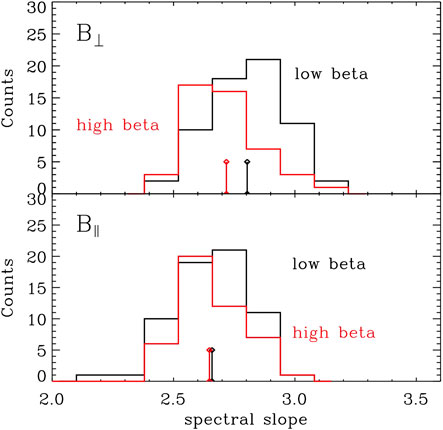
FIGURE 5. Spectral slope measured for different beta conditions in Cluster data; (black) $\beta <2$ and (red) $\beta >2$. Top panel refers to the spectrum of the perpendicular magnetic component $B_{\perp }$ and the bottom panel to $B_{\parallel }$. The short vertical lines ending with a diamond indicate average values of the histograms.

Moreover, a consequence of the behavior in Figure 5 is that while at high beta, $\delta B_{\parallel }$ and $\delta B_{\perp }$ have basically the same scaling, so that their ratio remains approximately constant in the sub‐ion range, at lower β, their slightly different scaling is expected to result in a slow increase of the $\delta B_{\parallel }/\delta B_{\perp }$ ratio between ion and electron scales. These properties are related to the evolution of the magnetic compressibility of the fluctuations in the sub‐ion range, which is the main focus of the next section.

5. Magnetic Compressibility

We now investigate the role of the third magnetic field component $B_z$, which is aligned with the local (at 4 s) magnetic field $B_0$. In particular, we focus on the magnetic compressibility $C_{\parallel }=\delta B_{\parallel }^2/\delta B^2$, where $\delta B^2=\delta B_{\parallel }^2+\delta B_{\perp }^2$, and its implication for the nature of the cascade at these scales. Note that, in this case, the measurement of $B_z$ is not affected by the sampling direction (provided that this is orthogonal to $B_0$ to a good approximation) and since we use the total perpendicular power $P_{\perp }$, the caution discussed in Section 4 is not needed here.

Figure 6 shows $C_{\parallel }$ for three intervals of different total β = 1,3,4 (${\beta }_p=0.3,1.4,2.5$) as measured from STAFF (red). For these three cases, we also show the spectrum of the magnetic field compressibility as measured at lower frequencies (corresponding to physical scales larger than $d_p$) by the FGM onboard Cluster (FGM, black). Note that FGM spectra are linearly interpolated between 0.14 and 0.4 Hz to remove artifacts due to spacecraft spin (0.25 Hz). There is a good matching between the two independent measurements at $f\sim 1$ Hz and where data points from both instruments are available for a more extended range, there is also a quite satisfactory overlap between them. The overall behavior agrees well with the expected picture: at a large scale, in the MHD inertial range, the level of compressibility is lower, typically $C_{\parallel }\mathrm{\lesssim }0.1$ (e.g., Horbury and Balogh, 2001; Smith et al., 2006), and starts to increase as approaching ion scales (Alexandrova et al., 2008; Hamilton et al., 2008; Salem et al., 2012; Kiyani et al., 2013; Roberts et al., 2017a), reaching sometimes variance isotropy (indicated by the dashed horizontal line) in the sub‐ion range, where the compressibility seems to be saturated. As already shown by Lacombe et al. (2017), the level of magnetic compressibility developed at small scales is larger for high beta than for small beta. Since we focus on the behavior at sub‐ion scales, in the following, we restrict our analysis to STAFF measurements only.

FIGURE 6

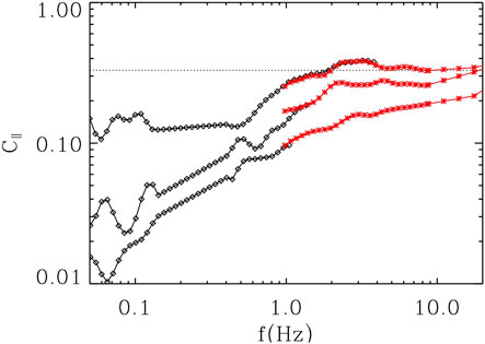
FIGURE 6. Examples of Cluster FGM (black) and STAFF (red) spectra of magnetic compressibility $C_{\parallel }$ as a function of the frequency measured in the spacecraft frame.

To highlight further the β-dependence of the magnetic compressibility, Figure 7 shows $C_{\parallel }$ for a selection of spectra with different β, increasing from red to purple. There is a continuous transition from lower to higher magnetic compressibility as a function of beta, in agreement with linear theory expectations (e.g., Podesta and TenBarge, 2012). Moreover, at high beta, it seems that the fluctuations reach an asymptotic $\delta B_{\parallel }^2/\delta B^2$ ratio, leading to an extended plateau in the spectrum, while at the lowest beta, a plateau cannot be clearly identified. We now want to identify more in detail what process and length scale control the level of $C_{\parallel }$ and in solar wind data.

FIGURE 7

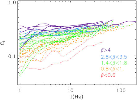
FIGURE 7. STAFF spectra of magnetic compressibility $C_{\parallel }$ as a function of the frequency measured in the spacecraft frame. Different colors and lines identify different groups of intervals with given β.

5.1. Beta Dependence and Theoretical Predictions

First, it is useful to go again from frequency to k-vector spectra: in Figure 8, frequencies are converted into k-vectors and normalized with respect to the proton inertial length $d_p$.

FIGURE 8

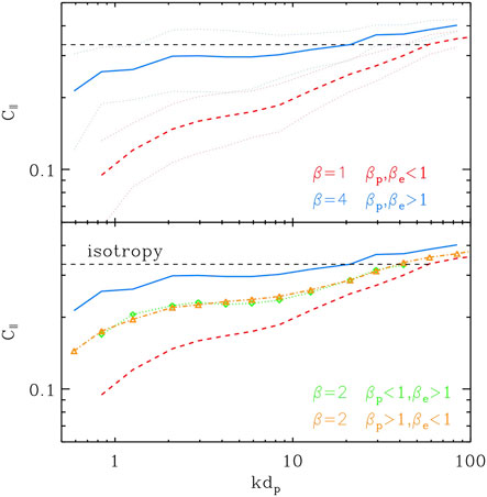
FIGURE 8. Cluster average spectra of magnetic compressibility for intervals with ${\beta }_e$ and ${\beta }_p<1$ (red) and ${\beta }_e$ and ${\beta }_p>1$ (blue); in the bottom panel, intermediate values with similar average β but with ${\beta }_p<1$, ${\beta }_e>1$, and ${\beta }_p>1$, ${\beta }_e<1$ are also shown in green and orange, respectively. Thin dotted lines in the upper panel show the one-sigma dispersion of the data.

We first identify two big categories such that both proton and electron betas are small, i.e., ${\beta }_p<1$ and ${\beta }_e<1$, or both are large, i.e., ${\beta }_p>1$ and ${\beta }_e>1$. We obtain an average total beta $\beta \sim 1$ in the former and $\beta \sim 4$ in the latter. The average spectrum of magnetic compressibility for each of the two families is shown in the top panel of Figure 8 as a function of $k{d}_p$; the thin dotted lines identify the standard deviation around the averages. In the high beta case (solid blue), the compressibility reaches a plateau after $k{d}_p=1$ and is saturated at an average level which is very close to isotropy (same power in $P_x,P_y$, and $P_z$), while in the low beta case (dashed red), $C_{\parallel }$ remains smaller and there is not a clear plateau at $k{d}_p>1$.

The remaining spectra are further separated in two other families: the first with ${\beta }_p<1$ and ${\beta }_e>1$ and the second with ${\beta }_p>1$ and ${\beta }_e<1$. In this case, the average total betas are very similar, $\beta \sim 1.9$ (${\beta }_p\sim 0.75$) and $\beta \sim 2.0$ (${\beta }_p\sim 1.5$), respectively, and fall in between the other two groups (small and large β). Consistent with this, the average spectrum of these two families, shown in orange and green in the bottom panel, has a level of compressibility at sub‐ion scales that is intermediate with respect to the other two curves. Moreover, they almost precisely fall on top of each other. All this suggests that not only is the total plasma beta a good parameter for ordering the level of compressibility generated at sub‐ion scales, but also this level is roughly independent of the individual weights of ${\beta }_p$ and ${\beta }_e$, being their sum $\beta ={\beta }_p+{\beta }_e$ the only relevant parameter.

This observational finding is in very good agreement with the expectation from the following relation:

$C_{\parallel }=\frac{{\beta }_p/2\left(1+T_e/T_p\right)}{1+{\beta }_p\left(1+T_e/T_p\right)}=\frac{\beta /2}{1+\beta },(2)$

where $T_e$ and $T_p$ are the electron and proton temperatures.

Eq. 2 can be derived (Schekochihin et al., 2009; Boldyrev et al., 2013) under the assumption of low-frequency magnetic structures in pressure balance at scales where the ion velocity becomes negligible compared to the electron one, or equivalently, the Hall term $\mathit{J}\times \mathit{B}$ becomes dominant over the ideal MHD term $-\mathit{U}\times \mathit{B}$. A special case is the regime of KAW, however, Eq. 2, which does not depend explicitly on k and thus on a specific dispersion relation, can be seen as a more general condition for highly oblique fluctuations in the sub‐ion range (e.g., ion-scale Alfvénic vortices, Jovanovic et al., 2020), under the assumptions described above (see e.g., Appendix C2 of Schekochihin et al., 2009).

5.2. Comparison with Simulations

To improve our analysis, we focus more in detail on the Cluster observations and compare them with numerical results. Note that, as in the simulations of Franci et al. (2016), it is only considered the case ${\beta }_p={\beta }_e$; we have made a selection of solar wind spectra with similar properties (${\beta }_p\sim {\beta }_e\sim \beta /2$). These have then been divided in five subgroups as a function of β and averaged to obtain a mean $C_{\parallel }$ profile for each β-family. The selection results in 7, 13, 23, 9, and 1 spectra for $\beta =0.6,\mathrm{1,2,4,8}$, respectively (only one spectrum fulfills the condition for high enough beta). Simulations with approximatively the same ${\beta }_p$ (and β) are considered for a direct comparison. In the following analysis, we want to identify the physical scale associated with the changes in the properties of the fluctuations and its possible connection to either the ion Larmor radius ${\rho }_p$ or the inertial length $d_p$, as they are related by ${\rho }_p=\sqrt{{\beta }_p}{d}_p$.

The results of this comparison are shown in Figure 9, where scales are normalized to both $d_p$ (top) and ${\rho }_p$ (bottom). Left panels show spectra from in situ data and right panels result from simulations, where the colors encode the same range of β. Qualitatively, the global trend seen in the simulations matches well that of the observations. First, the level of magnetic compressibility reached sub‐ion scales increases monotonically with β, as expected. Second, we can identify a plateau phase beyond ion scales whose extension is gradually reduced as β decreases; for the smallest betas, the plateau disappears and is replaced by an almost monotonic increase of $C_{\parallel }$ all along the sub‐ion range, though with a shallower slope compared to that of the transition from the MHD range.

FIGURE 9

FIGURE 9. Top panels (left): Cluster spectra of magnetic compressibility for intervals binned on different β, encoded in different styles and colors. Only cases with ${\beta }_p\sim {\beta }_e$ have been retained. The horizontal dashed line denotes energy equipartition between components (i.e., isotropy). Right: spectra of magnetic compressibility for simulations with different ${\beta }_p={\beta }_e$, shown with the same style as the left panel. The increase of $C_{\parallel }$ for $k{d}_i\gtrsim 8$ is due to numerical noise. Bottom: the same as top panels, but with k-vectors normalized with respect to the ion gyroradius ${\rho }_p$. Horizontal dotted lines, colored according to their β, are the theoretical prediction of $C_{\parallel }$ from Eq. 2.

This seems to suggest a different behavior of the turbulent fluctuations populating the sub-ion cascade as a function of the beta. To investigate further this aspect, horizontal dotted lines in the right panels of Figure 9 show the theoretical prediction for the asymptotic level of $C_{\parallel }$ between ion and electron scales predicted by Eq. 2, with the same color scale. For simulations at large β, when a plateau is clearly observed, the level of magnetic compressibility also agrees well with the one predicted by the theory. In the low beta case, there is a larger discrepancy and the observed level of magnetic compressibility is larger than the constant level predicted by Eq. 2. The different behavior of the compressibility in low- and high beta regimes found in our simulations, together with the larger discrepancy with respect to the theoretical predictions observed at low beta, is also consistent with results from previous numerical studies (e.g., Cerri et al., 2016; Cerri et al., 2017; Grošelj et al., 2017).

The situation is somewhat different when comparing predictions to the in situ data; in this case, there is a slight difference between the KAW level and the observed one, and this is persistent at all β. In particular, at high beta, it is apparent that while Eq. 2 predicts compressibility that goes beyond 1/3 (for $\beta \to \infty$, we have $C_{\parallel }=0.5$, so $\delta B_{\parallel }=\delta B_{\perp }$), a condition well recovered in the simulations, in Cluster data $C_{\parallel }$, does not go beyond component isotropy ($\delta B_{\parallel }=\delta B_{\perp }/2$; thus, $C_{\parallel }=1/3$). However, due to the low statistics in the data (just one spectrum has $\beta \gtrsim 8$), it is hard to draw a firm conclusion here.

Interestingly, from Figure 9, it seems that neither $d_p$ nor ${\rho }_p$ is able to fully capture and order the change in the spectrum of the magnetic compressibility for different betas; the saturation/plateau phase for low β spectra results more shifted toward high k-vectors compared to the high β ones when normalizing to $d_p$, while the vice versa is observed when normalizing to ${\rho }_p$. This suggests that the behavior can be better captured by an intermediate scale between the two. For this reason, in Figure 10, we have normalized spectra on a mixed scale $\sqrt{d_p{\rho }_p}$. Note that such a scale, proportional to $d_p{\beta }_p^{1/4}$, was found to describe well the behavior of the ion-break scale in magnetic field spectra in the range ${\beta }_p\sim 1$ by Franci et al. (2016), and, although not shown, to describe the variation of the break of the parallel magnetic field spectrum at all betas; this then motivated our choice. When such a mixed scale is used (top right panel), all cases follow the same trend: they grow until they reach $k\sqrt{d_p{\rho }_p}\sim 2$ and then start flattening, the saturation level depending on the beta. In situ observations (top left panel) seem to follow the same trend, confirming that such an intermediate scale is a good candidate for controlling the variation of the magnetic compressibility spectrum at ion scales.

FIGURE 10

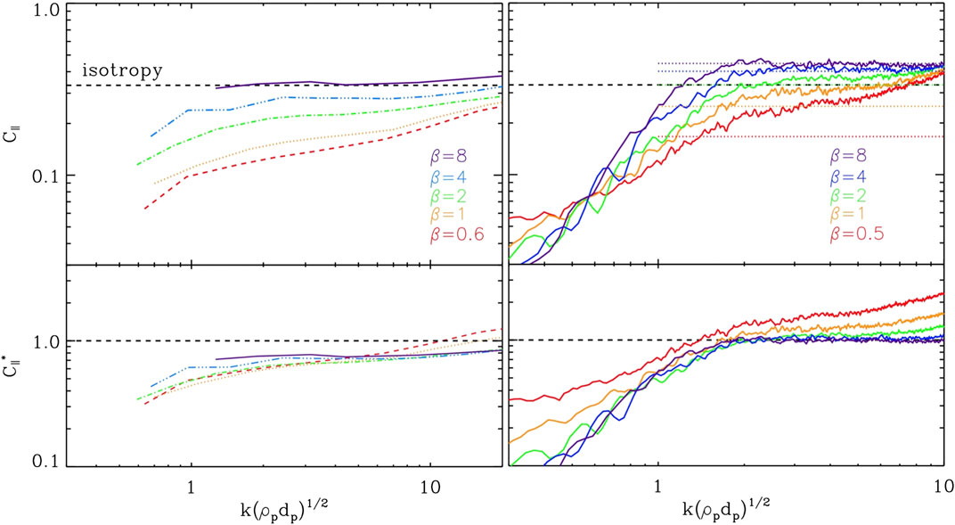
FIGURE 10. The same spectra as in Figure 9, but with k-vectors normalized to the mixed scale $\sqrt{d_p{\rho }_p}$; in the bottom panels, $C_{\parallel }$ is normalized to the theoretical prediction by Eq. 2.

It is then reasonable to use such a k-vector normalization to better evaluate the agreement with Eq. 2. In the bottom panels of the same figure $C_{\parallel }^{\text{*}}$, spectra are then normalized to the theoretical prediction for $C_{\parallel }$. In simulations, as already pointed out, cases with $\beta >1$ display a good agreement with the sub‐ion compressibility level predicted by the theory; as a consequence, when normalized to $\sqrt{d_p{\rho }_p}$, all spectra collapse on top of each other all along ion and sub‐ion scales. A worse agreement is observed at $\beta \le 1$ when simulations display a slightly higher compressibility level than predicted. Quite differently, the ratio between the in situ observations and the theoretical $C_{\parallel }$ is always below one and around 0.7–0.8 for all β groups in the sub‐ion range (see also Figure 10 of Lacombe et al., 2017). This behavior is consistent with the results of Pitňa et al. (2019) based on observations from the wind spacecraft, who find on average $C_{\parallel }\sim 0.9$, without making a distinction among beta regimes and with most of the data displaying a slightly smaller magnetic compressibility than the prediction. Our study confirms this scenario and suggests that the same trend is followed for all spectra, almost independently of the plasma beta. A ratio smaller than one and close to $\sim 0.75$ is also consistent with similar observational results of the plasma compressibility and based on the ratio between density and perpendicular magnetic fluctuations predicted by linear theory (Chen et al., 2013a; Pitňa et al., 2019). This was interpreted by Chen et al. (2013a) as a consequence of the nonlinear behavior of the solar wind fluctuations in the sub‐ion range, in agreement with simulations of strong KAW-turbulence (Boldyrev et al., 2013). On the other hand, for the magnetic compressibility, our fully nonlinear simulations of sub‐ion turbulence do not recover the same effect seen in situ, as $C_{\parallel }^{\text{*}}\mathrm{\gtrsim }1$. Other reasons could explain such a discrepancy, e.g., the effect of some electron Landau damping on the fluctuations observed in situ (Howes et al., 2011; Passot and Sulem, 2015; Schreiner and Saur, 2017) and not captured by the hybrid model. In order to answer these questions, a more detailed study of the polarization properties of the fluctuations in our simulations is in preparation.

Finally, note that the increase in $C_{\parallel }$ observed at higher k in the in situ data could be related to a further change in the properties of the fluctuations as they approach electron scales; as discussed in Lacombe et al. (2017), this also coincides with a change in the estimated spectral anisotropy. For example, Chen and Boldyrev (2017) have suggested that the increase in the magnetic compressibility beyond the sub‐ion range could be related to electron inertia corrections to Eq. 2. This effect is then not captured by the hybrid model and we cannot compare any more the observations with the simulations in this range. It is however interesting to note that while the further increase of compressibility at electron scales is predicted for ${\beta }_e\mathrm{\lesssim }1$ (Chen and Boldyrev, 2017; Passot et al., 2017), in the intervals measured by Cluster, it seems to be observed for all beta ranges for $k{d}_p\mathrm{\gtrsim }10$ ($k{d}_e\mathrm{\gtrsim }1/4$). Moreover, it is also interesting to note that spectra for all betas reach isotropy at roughly $k{\rho }_p\sim 20$, corresponding on average to $k{\rho }_e\sim 0.5$.

6. Conclusion

In summary, we have discussed the properties of magnetic field spectra of turbulent fluctuations in the sub‐ion regime and their main dependence on the plasma beta. We have carried out a detailed comparison between in situ Cluster magnetic field observations in the frequency range f(Hz)$=\left[\mathrm{1,200}\right]$, corresponding to scales typically between $d_p<l<d_e$, and high-resolution 2D hybrid simulations.

First, we investigated the spectral anisotropy of magnetic fluctuations at sub‐ion scales. Our simulations confirm that the model of Saur and Bieber (1999), originally developed for MHD range fluctuations, is valid also at kinetic scales; by applying the model to the numerical spectra obtained mimicking the sampling along a fixed direction made by spacecraft, we were able to successfully capture original spectral properties as well as their variation with β. This then reinforces the finding of Lacombe et al. (2017) who applied the Saur and Bieber model to kinetic-scale observations for the first time and concluded that fluctuations of the solar wind spectrum in the sub‐ion range are quasi-2D and gyrotropic. Moreover, we have shown that the component anisotropy measured in situ — leading to an apparent nongyrotropic spectrum from an original gyrotropic one (see also Turner et al., 2011) — is a direct consequence of the solenoidal condition of the magnetic field and the sampling procedure. This is not an effect related to the Doppler-shift of k-vectors swept through the spacecraft by the fast plasma flow and in fact, we were able to reproduce it in simulations just imposing a fixed sampling direction.

Note that our result about the global 2D-symmetry of the k-vectors around the magnetic field is not inconsistent with studies addressing the local shape of the eddies and suggesting the presence of a 3D anisotropy (e.g., Chen et al., 2012a; Verdini and Grappin, 2015; Verdini et al., 2018; Verdini et al., 2019; Wang et al., 2020). In our approach, we do not consider the specific orientation of the turbulent structures in the plane perpendicular to B, and it is reasonable to expect that the local 3D anisotropy is then lost. In other words, despite the 3D anisotropy of the turbulent eddies, their k-vectors can be oriented isotropically around B, leading then—in a frame like the one used here—to the 2D spectrum found in the Cluster observations. This does not exclude that some aspects of the 3D anisotropy could still be captured using a global approach; however, our study suggests that, in this case, one has to also carefully take into account the effects of the component anisotropy introduced by the sampling (Saur and Bieber, 1999, see also Figure 3 in this work).

For the magnetic compressibility $C_{\parallel }$, we have confirmed that it has a strong dependence on the plasma beta (e.g., Alexandrova et al., 2008; TenBarge et al., 2012; Lacombe et al., 2017). In particular, we have shown that in Cluster observations $C_{\parallel }$ depends on the total beta β only (Figure 8), as expected for low-frequency pressure-balanced fluctuations at highly oblique propagation (e.g., KAW). In the β range explored, we find a good qualitative agreement between the trends observed in the data and in the simulations. The compressibility is observed to increase as a function of β, leading to a plateau at sub‐ion scales for high betas and in good agreement with the prediction by Eq. 2. At low beta, a fully developed plateau is not observed beyond ion scales and the compressibility continues to slowly increase along sub‐ion scales, in both observations and simulations (see also Grošelj et al., 2019). There is, however, a difference in the asymptotic level of compressibility reached at high β in data and our simulations; in the former, fluctuations seem not to exceed component isotropy ($C_{\parallel }=1/3$), while in the latter, they approach $C_{\parallel }=0.5$, which is the limiting value predicted by Eq. 2. This aspect deserves to be explored in future studies, extending the range of β explored, to then establish if the asymptotic condition observed in simulations and predicted by the theory, which implies the same power in the parallel component as in the sum of the perpendicular ones, can be also observed in situ for high enough β intervals. As a consequence of the behavior just described, there is a different quantitative agreement of the magnetic compressibility observed in situ and in simulations, with the theoretical prediction by Eq. 2. In simulations, there is very good matching with the predicted level at higher beta, but an excess of $C_{\parallel }$ at low beta; this effect was already observed in Cerri et al. (2017) and is confirmed here on a larger range of β. On the other hand, in solar wind observations, the ratio is always lower than 1 (smaller compressibility than predicted by the theory) and close to $\sim 0.75$ for all β, in agreement with similar studies on the plasma compressibility (Chen et al., 2013a; Pitňa et al., 2019).

Our analysis also suggests that the increase in the compressibility at ion scales is controlled by an intermediate scale between the Larmor radius ${\rho }_p$ and the proton inertial length $d_p$ (Figure 9). For simulations, this was already anticipated in Franci et al. (2016), and we could identify it as related to $\sqrt{d_p{\rho }_p}$, thus proportional to $d_p{\beta }_p^{1/4}$ (Figure 10). Such a scaling with ${\beta }_p$ also corresponds to the scaling observed for the spectral ion break in the range ${\beta }_p\sim 1$. However, it is worth highlighting that both observations (Chen et al., 2014; Wang et al., 2018; Woodham et al., 2018) and our simulations (Franci et al., 2016) show that the spectral ion-break scale follows the largest of ${\rho }_p$ and $d_p$ depending on the beta, so that the correction term proportional to $d_p{\beta }_p^{1/4}$ identified in Franci et al. (2016) is important only around ${\beta }_p\sim 1$. On the other hand, the present study indicates that a scale proportional to $\sqrt{d_p{\rho }_p}$ orders well the spectra of compressibility at all betas, for both in situ data and simulations, suggesting that such a mixed scale controls the transition in the nature of the fluctuations from MHD to sub‐ion range (see also the monotonic scaling with ${\beta }_p$ of the ion break in the parallel magnetic field spectrum shown in Figure 4 of Franci et al., 2016). This may imply that the two changes of the regime—the steepening of the magnetic spectrum and the increase in the compressibility—can occur at different scales for more extreme β values. In particular, we expect the spectral break to occur at a larger scale with respect to the plateau in the compressibility when ${\beta }_p\gg 1$ or ${\beta }_p\ll 1$, as in these cases, $\sqrt{d_p{\rho }_p}$ is always smaller than the largest between ${\rho }_p$ and $d_p$. A more detailed analysis on this aspect will be the subject of a future study, as well as the possible implications of this behavior for fluctuations in the inner Heliosphere, where the plasma beta is typically lower than at 1AU, which can be observed by the Parker Solar Probe and Solar Obiter.

Data Availability Statement

Publicly available datasets were analyzed in this study. This data can be found here: ESA Cluster archive: https://csa.esac.esa.int The numerical data are available at https://b2share.eudat.eu/records/a58135af9c9d429f92c15ce88bdfdd55.

Author Contributions

LM and LF performed the main analysis and produced figures. OA and CL identified Cluster intervals, provided the in situ dataset, and contributed to the observational spectral analysis. PH provided the hybrid code, LF performed the numerical simulations, and together with LM, SL, AV, and EP, they discussed the use and interpretation of numerical data. All authors contributed to the global interpretation of the results, as well as to their discussion and presentation in the manuscript. All authors revised the manuscript before submission.

Funding

This work was supported by the Programme National PNST of CNRS/INSU co-funded by CNES. It has also been funded by Fondazione Cassa di Risparmio di Firenze through the project HYPERCRHEL. LF was supported by Fondazione Cassa di Risparmio di Firenze, through the project Giovani Ricercatori Protagonisti, and by the United Kingdom Science and Technology Facilities Council (STFC) grants ST/P000622/1 and ST/T00018X/1. PH acknowledges grant 18-08861S of the Czech Science Foundation. OA and CL are supported by the French Centre National d’Etude Spatiales (CNES).

Conflict of Interest

The authors declare that the research was conducted in the absence of any commercial or financial relationships that could be construed as a potential conflict of interest.

The reviewer (SC) declared a past co-authorship with one of the authors (LF) to the handling Editor.

Acknowledgments

The authors acknowledge useful discussions with J. Stawarz, G. Howes, and A. Pitna. The authors acknowledge PRACE for awarding them access to resource Cartesius based in the Netherlands at SURFsara through the DECI-13 (Distributed European Computing Initiative) call (project HybTurb3D), and CINECA for the availability of high performance computing resources and support under the ISCRA initiative (grants HP10C877C4 and HP10BUUOJM) and the program Accordo Quadro INAF-CINECA 2017-2019 (grants C4A26 and C3A22a).

Appendix: Symbol Definitions and Normalized Units

The subscripts $\perp$ and $\parallel$ refer to the direction with respect to the ambient magnetic field ${\mathit{B}}_0$ and p and e denote, respectively, protons and electrons. All equations are expressed in the c.g.s. unity system. n and T denote the number density and the temperature of a species (we assume also $n_p=n_e=n$). ${\beta }_{e,p}=8\pi n{k}_B{T}_{e,p}/B_0^2$ are the electron and proton betas, and $\beta ={\beta }_p+{\beta }_e$ is the total plasma beta; here $k_B$ is the Boltzmann constant. For each species of mass m and charge q, the inertial length d is defined as $c/{\omega }_p$, where ${\omega }_p={\left(4\pi n{q}^2/m\right)}^{1/2}$ is the plasma frequency, and the Larmor radius ρ is defined as $v_{th}/{\text{Ω}}_c$, where $v_{th}$ it the thermal speed of each species and ${\text{Ω}}_c=q_p{B}_o/mc$ is the cyclotron frequency. $V_{sw}$ is the solar wind speed and f the frequency of the fluctuations measured by the spacecraft; k denotes the module of the wave vector $\mathit{k}$.

References

Alexandrova, O., Krishna Jagarlamudi, V., Rossi, C., Maksimovic, M., Hellinger, P., Shprits, Y., et al. (2020). Kinetic turbulence in space plasmas observed in the near-Earth and near-Sun solar wind. arXiv e-prints arXiv: 2004.01102

Google Scholar

Alexandrova, O., Lacombe, C., Mangeney, A., Grappin, R., and Maksimovic, M. (2012). Solar wind turbulent spectrum at plasma kinetic scales. Astrophys. J. 760, 121. doi:10.1088/0004-637X/760/2/121

CrossRef Full Text | Google Scholar

Alexandrova, O., Lacombe, C., and Mangeney, A. (2008). Spectra and anisotropy of magnetic fluctuations in the Earth’s magnetosheath: Cluster observations. Ann. Geophys. 26, 3585–3596. doi:10.5194/angeo-26-3585-2008

CrossRef Full Text | Google Scholar

Alexandrova, O., Saur, J., Lacombe, C., Mangeney, A., Mitchell, J., Schwartz, S. J., et al. (2009). Universality of solar-wind turbulent spectrum from MHD to electron scales. Phys. Rev. Lett. 103, 165003. doi:10.1103/PhysRevLett.103.165003

PubMed Abstract | CrossRef Full Text | Google Scholar

Arzamasskiy, L., Kunz, M. W., Chandran, B. D. G., and Quataert, E. (2019). Hybrid-kinetic simulations of ion heating in alfvénic turbulence. Astrophys. J. 879, 53. doi:10.3847/1538-4357/ab20cc

CrossRef Full Text | Google Scholar

Bandyopadhyay, R., Sorriso-Valvo, L., Chasapis, A. r., Hellinger, P., Matthaeus, W. H., Verdini, A., et al. (2020). In Situ observation of hall magnetohydrodynamic cascade in space plasma. Phys. Rev. Lett. 124, 225101. doi:10.1103/PhysRevLett.124.225101

PubMed Abstract | CrossRef Full Text | Google Scholar

Bieber, J. W., Wanner, W., and Matthaeus, W. H. (1996). Dominant two-dimensional solar wind turbulence with implications for cosmic ray transport. J. Geophys. Res. 101, 2511–2522. doi:10.1029/95JA02588

CrossRef Full Text | Google Scholar

Biskamp, D., Schwarz, E., and Drake, J. F. (1996). Two-dimensional electron magnetohydrodynamic turbulence. Phys. Rev. Lett. 76, 1264–1267. doi:10.1103/PhysRevLett.76.1264

PubMed Abstract | CrossRef Full Text | Google Scholar

Boldyrev, S., Horaites, K., Xia, Q., and Perez, J. C. (2013). Toward a theory of astrophysical plasma turbulence at subproton scales. Astrophys. J 777, 41. doi:10.1088/0004-637X/777/1/41

CrossRef Full Text | Google Scholar

Boldyrev, S., and Perez, J. C. (2012). Spectrum of kinetic-alfvén turbulence. Astrophys. J. Lett. 758, L44. doi:10.1088/2041-8205/758/2/L44

CrossRef Full Text | Google Scholar

Bruno, R., and Carbone, V. (2013). The solar wind as a turbulence laboratory. Living Rev. Sol. Phys. 10, 2. doi:10.12942/lrsp-2013-2

CrossRef Full Text | Google Scholar

Cerri, S. S., Califano, F., Jenko, F., Told, D., and Rincon, F. (2016). Subproton-scale cascades in solar wind turbulence: driven hybrid-kinetic simulations. Astrophys. J. Lett. 822, L12. doi:10.3847/2041-8205/822/1/L12

CrossRef Full Text | Google Scholar

Cerri, S. S., Grošelj, D., and Franci, L. (2019). Kinetic plasma turbulence: recent insights and open questions from 3D3V simulations. Front. Astron. Space Sci. 6, 64. doi:10.3389/fspas.2019.00064

CrossRef Full Text | Google Scholar

Cerri, S. S., Kunz, M. W., and Califano, F. (2018). Dual phase-space cascades in 3D hybrid-vlasov-maxwell turbulence. Astrophys. J. Lett. 856, L13. doi:10.3847/2041-8213/aab557

CrossRef Full Text | Google Scholar

Cerri, S. S., Servidio, S., and Califano, F. (2017). Kinetic cascade in solar-wind turbulence: 3D3V hybrid-kinetic simulations with electron inertia. Astrophys. J. Lett. 846, L18. doi:10.3847/2041-8213/aa87b0

CrossRef Full Text | Google Scholar

Chen, C. H. K., Bale, S. D., Salem, C. S., and Maruca, B. A. (2013a). Residual energy spectrum of solar wind turbulence. Astrophys. J. 770, 125. doi:10.1088/0004-637X/770/2/125

CrossRef Full Text | Google Scholar

Chen, C. H. K., and Boldyrev, S. (2017). Nature of kinetic scale turbulence in the Earth’s magnetosheath. Astrophys. J. 842, 122. doi:10.3847/1538-4357/aa74e0

CrossRef Full Text | Google Scholar

Chen, C. H. K., Boldyrev, S., Xia, Q., and Perez, J. C. (2013b). Nature of subproton scale turbulence in the solar wind. Phys. Rev. Lett. 110, 225002. doi:10.1103/PhysRevLett.110.225002

PubMed Abstract | CrossRef Full Text | Google Scholar

Chen, C. H. K., Horbury, T. S., Schekochihin, A. A., Wicks, R. T., Alexandrova, O., and Mitchell, J. (2010). Anisotropy of solar wind turbulence between ion and electron scales. Phys. Rev. Lett. 104, 255002. doi:10.1103/PhysRevLett.104.255002

CrossRef Full Text | Google Scholar

Chen, C. H. K., Leung, L., Boldyrev, S., Maruca, B. A., and Bale, S. D. (2014). Ion-scale spectral break of solar wind turbulence at high and low beta. Geophys. Res. Let. 41, 8081–8088. doi:10.1002/2014GL062009

CrossRef Full Text | Google Scholar

Chen, C. H. K., Mallet, A., Schekochihin, A. A., Horbury, T. S., Wicks, R. T., and Bale, S. D. (2012a). Three-dimensional structure of solar wind turbulence. Astrophys. J. 758, 120. doi:10.1088/0004-637X/758/2/120

CrossRef Full Text | Google Scholar

Chen, C. H. K., Salem, C. S., Bonnell, J. W., Mozer, F. S., and Bale, S. D. (2012b). Density fluctuation spectrum of solar wind turbulence between ion and electron scales. Phys. Rev. Lett. 109, 035001. doi:10.1103/PhysRevLett.109.035001

CrossRef Full Text | Google Scholar

Chen, C. H. K. (2016). Recent progress in astrophysical plasma turbulence from solar wind observations. J. Plasma Phys. 82, 535820602. doi:10.1017/S0022377816001124

CrossRef Full Text | Google Scholar

Dasso, S., Milano, L. J., Matthaeus, W. H., and Smith, C. W. (2005). Anisotropy in fast and slow solar wind fluctuations. Astrophys. J. 635, L181–L184. doi:10.1086/499559

CrossRef Full Text | Google Scholar

Franci, L., Hellinger, P., Guarrasi, M., Chen, C. H. K., Papini, E., Verdini, A., et al. (2018a). Three-dimensional simulations of solar wind turbulence with the hybrid code CAMELIA. J. Phys. Conf. Ser. 1031, 012002. doi:10.1088/1742-6596/1031/1/012002

CrossRef Full Text | Google Scholar

Franci, L., Landi, S., Verdini, A., Matteini, L., and Hellinger, P. (2018b). Solar wind turbulent cascade from MHD to sub-ion scales: large-size 3D hybrid particle-in-cell simulations. Astrophys. J. 853, 26. doi:10.3847/1538-4357/aaa3e8

CrossRef Full Text | Google Scholar

Franci, L., Landi, S., Matteini, L., Verdini, A., and Hellinger, P. (2015a). High-resolution hybrid simulations of kinetic plasma turbulence at proton scales. Astrophys. J. 812, 21. doi:10.1088/0004-637X/812/1/21

CrossRef Full Text | Google Scholar

Franci, L., Verdini, A., Matteini, L., Landi, S., and Hellinger, P. (2015b). Solar wind turbulence from MHD to sub-ion scales: high-resolution hybrid simulations. Astrophys. J. Lett. 804, L39. doi:10.1088/2041-8205/804/2/L39

CrossRef Full Text | Google Scholar

Franci, L., Landi, S., Matteini, L., Verdini, A., and Hellinger, P. (2016). Plasma beta dependence of the ion-scale spectral break of solar wind turbulence: high-resolution 2D hybrid simulations. Astrophys. J. 833, 91. doi:10.3847/1538-4357/833/1/91

CrossRef Full Text | Google Scholar

Grošelj, D., Cerri, S. S., Bañón Navarro, A., Willmott, C., Told, D., Loureiro, N. F., et al. (2017). Fully kinetic versus reduced-kinetic modeling of collisionless plasma turbulence. Astrophys. J. 847, 28. doi:10.3847/1538-4357/aa894d

CrossRef Full Text | Google Scholar

Grošelj, D., Chen, C. H. K., Mallet, A., Samtaney, R., Schneider, K., and Jenko, F. (2019). Kinetic turbulence in astrophysical plasmas: waves and/or structures? Phys. Rev. X 9, 031037. doi:10.1103/PhysRevX.9.031037

CrossRef Full Text | Google Scholar

Hamilton, K., Smith, C. W., Vasquez, B. J., and Leamon, R. J. (2008). Anisotropies and helicities in the solar wind inertial and dissipation ranges at 1 AU. J. Geophys. Res. Space Phys. 113, A01106. doi:10.1029/2007JA012559

CrossRef Full Text | Google Scholar

Hellinger, P., Landi, S., Matteini, L., Verdini, A., and Franci, L. (2017). Mirror instability in the turbulent solar wind. Astrophys. J. 838, 158. doi:10.3847/1538-4357/aa67e0

CrossRef Full Text | Google Scholar

Hellinger, P., Matteini, L., Landi, S., Verdini, A., Franci, L., and Travnicek, P. M. (2015). Plasma turbulence and kinetic instabilities at ion scales in the expanding solar wind. Astrophys. J. Lett. 811, L32

Google Scholar

Hellinger, P., Verdini, A., Landi, S., Franci, L., and Matteini, L. (2018). von Kármán-Howarth equation for Hall magnetohydrodynamics: hybrid simulations. Astrophys. J. Lett. 857, L19. doi:10.3847/2041-8213/aabc06

CrossRef Full Text | Google Scholar

Horbury, T. S., and Balogh, A. (2001). Evolution of magnetic field fluctuations in high-speed solar wind streams: ulysses and Helios observations. J. Geophys. Res. 106, 15929–15940. doi:10.1029/2000JA000108

CrossRef Full Text | Google Scholar

Horbury, T. S., Forman, M., and Oughton, S. (2008). Anisotropic scaling of magnetohydrodynamic turbulence. Phys. Rev. Lett. 101, 175005. doi:10.1103/PhysRevLett.101.175005

CrossRef Full Text | Google Scholar

Howes, G. G., Dorland, W., Cowley, S. C., Hammett, G. W., Quataert, E., Schekochihin, A. A., et al. (2008). Kinetic simulations of magnetized turbulence in astrophysical plasmas. Phys. Rev. Lett. 100, 065004. doi:10.1103/PhysRevLett.100.065004

CrossRef Full Text | Google Scholar

Howes, G. G., Tenbarge, J. M., Dorland, W., Quataert, E., Schekochihin, A. A., Numata, R., et al. (2011). Gyrokinetic simulations of solar wind turbulence from ion to electron scales. Phys. Rev. Lett. 107, 035004. doi:10.1103/PhysRevLett.107.035004

CrossRef Full Text | Google Scholar

Howes, G. G. (2015). The inherently three-dimensional nature of magnetized plasma turbulence. J. Plasma Phys. 81, 325810203. doi:10.1017/S0022377814001056

CrossRef Full Text | Google Scholar

Jovanovic, D., Alexandrova, O., Maksimovic, M., and Belic, M. (2020). Fluid theory of coherent magnetic vortices in high-β space plasmas. Astrophys. J. 896 (1), 18. doi:10.3847/1538-4357/ab8a45

CrossRef Full Text | Google Scholar

Kiyani, K. H., Chapman, S. C., Khotyaintsev, Y. V., Dunlop, M. W., and Sahraoui, F. (2009). Global scale-invariant dissipation in collisionless plasma turbulence. Phys. Rev. Lett. 103, 075006. doi:10.1103/PhysRevLett.103.075006

CrossRef Full Text | Google Scholar

Kiyani, K. H., Chapman, S. C., Sahraoui, F., Hnat, B., Fauvarque, O., and Khotyaintsev, Y. V. (2013). Enhanced magnetic compressibility and isotropic scale invariance at sub-ion larmor scales in solar wind turbulence. Astrophys. J. 763, 10. doi:10.1088/0004-637X/763/1/10

CrossRef Full Text | Google Scholar

Lacombe, C., Alexandrova, O., and Matteini, L. (2017). Anisotropies of the magnetic field fluctuations at kinetic scales in the solar wind: cluster observations. Astrophys. J. 848, 45. doi:10.3847/1538-4357/aa8c06

CrossRef Full Text | Google Scholar

Landi, S., Franci, L., Papini, E., Verdini, A., Matteini, L., and Hellinger, P. (2019). Spectral anisotropies and intermittency of plasma turbulence at ion kinetic scales. arXiv eprint arXiv:1904.03903

Google Scholar

Loureiro, N. F., and Boldyrev, S. (2017). Collisionless reconnection in magnetohydrodynamic and kinetic turbulence. Astrophys. J. 850, 182. doi:10.3847/1538-4357/aa9754

CrossRef Full Text | Google Scholar

Mallet, A., Schekochihin, A. A., and Chandran, B. D. G. (2017). Disruption of sheet-like structures in Alfvénic turbulence by magnetic reconnection. Mon. Notices Royal Astron. Soc. 468, 4862–4871. doi:10.1093/mnras/stx670

CrossRef Full Text | Google Scholar

Matteini, L., Alexandrova, O., Chen, C. H. K., and Lacombe, C. (2017). Electric and magnetic spectra from MHD to electron scales in the magnetosheath. Mon. Notices Royal Astron. Soc. 466, 945–951. doi:10.1093/mnras/stw3163

CrossRef Full Text | Google Scholar

Matthaeus, W. H., Goldstein, M. L., and Roberts, D. A. (1990). Evidence for the presence of quasi-two-dimensional nearly incompressible fluctuations in the solar wind. J. Geophys. Res. 95, 20673–20683. doi:10.1029/JA095iA12p20673

CrossRef Full Text | Google Scholar

Matthews, A. P. (1994). Current advance method and cyclic leapfrog for 2d multispecies hybrid plasma simulations. J. Comp. Phys. 112, 102–116. doi:10.1006/jcph.1994.1084

CrossRef Full Text | Google Scholar

Osman, K. T., and Horbury, T. S. (2006). Multispacecraft measurement of anisotropic correlation functions in solar wind turbulence. Astrophys. J. 654, L103–L106. doi:10.1086/510906

CrossRef Full Text | Google Scholar

Papini, E., Franci, L., Landi, S., Verdini, A., Matteini, L., and Hellinger, P. (2019). Can Hall magnetohydrodynamics explain plasma turbulence at sub-ion scales? Astrophys. J. 870, 52. doi:10.3847/1538-4357/aaf003

CrossRef Full Text | Google Scholar

Parashar, T. N., Oughton, S., Matthaeus, W. H., and Wan, M. (2016). Variance anisotropy in kinetic plasmas. Astrophys. J. 824, 44. doi:10.3847/0004-637X/824/1/44

CrossRef Full Text | Google Scholar

Passot, T., and Sulem, P. L. (2015). A model for the non-universal power law of the solar wind sub-ion-scale magnetic spectrum. Astrophys. J. Lett. 812, L37. doi:10.1088/2041-8205/812/2/L37

CrossRef Full Text | Google Scholar

Passot, T., Sulem, P. L., and Tassi, E. (2017). Electron-scale reduced fluid models with gyroviscous effects. J. Plasma Phys. 83, 715830402. doi:10.1017/S0022377817000514

CrossRef Full Text | Google Scholar

Perrone, D., Alexandrova, O., Roberts, O. W., Lion, S., Lacombe, C., Walsh, A., et al. (2017). Coherent structures at ion scales in fast solar wind: cluster observations. Astrophys. J. 849, 49. doi:10.3847/1538-4357/aa9022

CrossRef Full Text | Google Scholar

Perrone, D., Valentini, F., Servidio, S., Dalena, S., and Veltri, P. (2013). Vlasov simulations of multi-ion plasma turbulence in the solar wind. Astrophys. J. 762, 99. doi:10.1088/0004-637X/762/2/99

CrossRef Full Text | Google Scholar

Pitňa, A., Šafránková, J., Němeček, Z., Franci, L., Pi, G., and Montagud Camps, V. (2019). Characteristics of solar wind fluctuations at and below ion scales. Astrophys. J. 879, 82. doi:10.3847/1538-4357/ab22b8

CrossRef Full Text | Google Scholar

Podesta, J. J., and TenBarge, J. M. (2012). Scale dependence of the variance anisotropy near the proton gyroradius scale: additional evidence for kinetic Alfvén waves in the solar wind at 1 AU. J. Geophys. Res. Space Phys.117, A10106. doi:10.1029/2012JA017724

CrossRef Full Text | Google Scholar

Roberts, O. W., Alexandrova, O., Kajdič, P., Turc, L., Perrone, D., Escoubet, C. P., et al. (2017a). Variability of the magnetic field power spectrum in the solar wind at electron scales. Astrophys. J. 850, 120. doi:10.3847/1538-4357/aa93e5

CrossRef Full Text | Google Scholar

Roberts, O. W., Narita, Y., and Escoubet, C. P. (2017b). Direct measurement of anisotropic and asymmetric wave vector spectrum in ion-scale solar wind turbulence. Astrophys. J. Lett. 851, L11. doi:10.3847/2041-8213/aa9bf3

CrossRef Full Text | Google Scholar

Šafránková, J., Němeček, Z., Přech, L., and Zastenker, G. N. (2013). Ion kinetic scale in the solar wind observed. Phys. Rev. Lett. 110, 025004. doi:10.1103/PhysRevLett.110.025004

CrossRef Full Text | Google Scholar

Sahraoui, F., Goldstein, M. L., Belmont, G., Canu, P., and Rezeau, L. (2010). Three dimensional anisotropic k spectra of turbulence at subproton scales in the solar wind. Phys. Rev. Lett. 105, 131101. doi:10.1103/PhysRevLett.105.131101

CrossRef Full Text | Google Scholar

Sahraoui, F., Huang, S. Y., Belmont, G., Goldstein, M. L., Rétino, A., Robert, P., et al. (2013). Scaling of the electron dissipation range of solar wind turbulence. Astrophys. J. 777, 15. doi:10.1088/0004-637X/777/1/15

CrossRef Full Text | Google Scholar

Salem, C. S., Howes, G. G., Sundkvist, D., Bale, S. D., Chaston, C. C., Chen, C. H. K., et al. (2012). Identification of kinetic Alfvén wave turbulence in the solar wind. Astrophys. J. Lett. 745, L9. doi:10.1088/2041-8205/745/1/L9

CrossRef Full Text | Google Scholar

Saur, J., and Bieber, J. W. (1999). Geometry of low-frequency solar wind magnetic turbulence: evidence for radially aligned Alfénic fluctuations. J. Geophys. Res. 104, 9975–9988. doi:10.1029/1998JA900077

CrossRef Full Text | Google Scholar

Schekochihin, A. A., Cowley, S. C., Dorland, W., Hammett, G. W., Howes, G. G., Quataert, E., et al. (2009). Astrophysical gyrokinetics: kinetic and fluid turbulent cascades in magnetized weakly collisional plasmas. Astrophys. J. Suppl. 182, 310–377. doi:10.1088/0067-0049/182/1/310

CrossRef Full Text | Google Scholar

Schreiner, A., and Saur, J. (2017). A model for dissipation of solar wind magnetic turbulence by kinetic Alfvén waves at electron scales: comparison with observations. Astrophys. J. 835, 133. doi:10.3847/1538-4357/835/2/133

CrossRef Full Text | Google Scholar

Smith, C. W., Vasquez, B. J., and Hamilton, K. (2006). Interplanetary magnetic fluctuation anisotropy in the inertial range. J. Geophys. Res. Space Phys. 111, A09111. doi:10.1029/2006JA011651

CrossRef Full Text | Google Scholar

Stawarz, J. E., Eriksson, S., Wilder, F. D., Ergun, R. E., Schwartz, S. J., Pouquet, A., et al. (2016). Observations of turbulence in a kelvin-helmholtz event on 8 september 2015 by the magnetospheric multiscale mission. J. Geophys. Res. 121 (11), 11021–11034. doi:10.1002/2016JA023458. 2016JA023458

CrossRef Full Text | Google Scholar

Stawarz, J. E., Matteini, L., Parashar, T. N., Franci, L., Eastwood, J. P., Gonzalez, C. A., et al. (2020). Generalized ohms law decomposition of the electric field in magnetosheath turbulence: magnetospheric multiscale observations. Earth and Space Science Open Archive. 31. doi:10.1002/essoar.10503618.1

CrossRef Full Text | Google Scholar

Sulem, P. L., Passot, T., Laveder, D., and Borgogno, D. (2016). Influence of the nonlinearity parameter on the solar wind sub-ion magnetic energy spectrum: FLR-Landau fluid simulations. Astrophys. J. 818, 66. doi:10.3847/0004-637X/818/1/66

CrossRef Full Text | Google Scholar

TenBarge, J. M., Podesta, J. J., Klein, K. G., and Howes, G. G. (2012). Interpreting magnetic variance anisotropy measurements in the solar wind. Astrophys. J. 753, 107. doi:10.1088/0004-637X/753/2/107

CrossRef Full Text | Google Scholar

Turner, A. J., Gogoberidze, G., Chapman, S. C., Hnat, B., and Müller, W. C. (2011). Nonaxisymmetric anisotropy of solar wind turbulence. Phys. Rev. Lett. 107, 095002. doi:10.1103/PhysRevLett.107.095002

CrossRef Full Text | Google Scholar

Valentini, F., Servidio, S., Perrone, D., Califano, F., Matthaeus, W. H., and Veltri, P. (2014). Hybrid Vlasov-Maxwell simulations of two-dimensional turbulence in plasmas. Phys. Plasmas. 21, 082307. doi:10.1063/1.4893301

CrossRef Full Text | Google Scholar

Verdini, A., and Grappin, R. (2015). Imprints of expansion on the local anisotropy of solar wind turbulence. Astrophys. J. Lett. 808, L34. doi:10.1088/2041-8205/808/2/L34

CrossRef Full Text | Google Scholar

Verdini, A., Grappin, R., Alexandrova, O., Franci, L., Landi, S., Matteini, L., et al. (2019). Three-dimensional local anisotropy of velocity fluctuations in the solar wind. Mon. Notices Royal Astron. Soc. 486, 3006–3018. doi:10.1093/mnras/stz1041

CrossRef Full Text | Google Scholar

Verdini, A., Grappin, R., Alexandrova, O., and Lion, S. (2018). 3D anisotropy of solar wind turbulence, tubes, or ribbons? Astrophys. J. 853, 85. doi:10.3847/1538-4357/aaa433

CrossRef Full Text | Google Scholar

Wang, T., He, J., Alexandrova, O., Dunlop, M., and Perrone, D. (2020). Observational quantification of three-dimensional anisotropies and scalings of space plasma turbulence at kinetic scales. Astrophys. J. 898, 91. doi:10.3847/1538-4357/ab99ca

CrossRef Full Text | Google Scholar

Wang, X., Tu, C., He, J., and Wang, L. (2018). On the full-range β dependence of ion-scale spectral break in the solar wind turbulence. Astrophys. J. 857, 136. doi:10.3847/1538-4357/aab960

CrossRef Full Text | Google Scholar

Wicks, R. T., Horbury, T. S., Chen, C. H. K., and Schekochihin, A. A. (2010). Power and spectral index anisotropy of the entire inertial range of turbulence in the fast solar wind. Mon. Notices Royal Astron. Soc. 407, L31–L35. doi:10.1111/j.1745-3933.2010.00898.x

CrossRef Full Text | Google Scholar

Woodham, L. D., Wicks, R. T., Verscharen, D., and Owen, C. J. (2018). The role of proton cyclotron resonance as a dissipation mechanism in solar wind turbulence: a statistical study at ion-kinetic scales. Astrophys. J. 856, 49. doi:10.3847/1538-4357/aab03d

CrossRef Full Text | Google Scholar