 Victor Réville1*
 Alexis P. Rouillard1Marco Velli2Andrea Verdini3
 Éric Buchlin4Michael Lavarra1Nicolas Poirier1
- 1IRAP, Université Toulouse III–Paul Sabatier, CNRS, CNES, Toulouse, France
- 2UCLA Earth Planetary and Space Sciences Department, Los Angeles, CA, United States
- 3Dipartimento di Fisica e Astronomia, Universitá di Firenze, Sesto Fiorentino, Italy
- 4Université Paris-Saclay, CNRS, Institut D’Astrophysique Spatiale, Orsay, France
The enrichment of coronal loops and the slow solar wind with elements that have low First Ionization Potential, known as the FIP effect, has often been interpreted as the tracer of a common origin. A current explanation for this FIP fractionation rests on the influence of ponderomotive forces and turbulent mixing acting at the top of the chromosphere. The implied wave transport and turbulence mechanisms are also key to wave-driven coronal heating and solar wind acceleration models. This work makes use of a shell turbulence model run on open and closed magnetic field lines of the solar corona to investigate with a unified approach the influence of magnetic topology, turbulence amplitude and dissipation on the FIP fractionation. We try in particular to assess whether there is a clear distinction between the FIP effect on closed and open field regions.
Introduction
The First Ionization Potential (FIP) effect is an enrichment of heavy elements with low-FIP such as Fe, Si, and Mg compared with photospheric abundances. It was initially measured in the solar wind and Solar Energetic Particles (SEPs) and later inferred from spectroscopic observations of the corona (see Meyer, 1985a, Meyer, 1985b; Bochsler et al., 1986; Gloeckler and Geiss, 1989; Feldman, 1992, and references therein). The FIP bias, i.e., the ratio of coronal to photospheric abundances, is moreover mass independent. This means that processes below the transition region are strongly affecting the hydrostatic balance of the partially ionized chromosphere. Early on, explanations of the FIP effect involved diffusion, flows or some sort of turbulent mixing in the chromosphere to prevent any gravitational settling (see, e.g., Marsch et al., 1995; Schwadron et al., 1999).
Schwadron et al. (1999) favored the hypothesis of turbulent wave heating in the chromosphere as a way to both prevent a mass-dependant fractionation and to obtain a low-FIP bias. Later on, Laming (2004) proposed the ponderomotive acceleration, i.e., the time averaged gradient of electromagnetic fluctuations, as the origin of the FIP effect. The ponderomotive acceleration has this advantage that it may change sign and could explain the inverse FIP effect observed in low-mass stars (Wood and Linsky, 2010; Laming, 2015). Both processes rely on Alfvén waves propagating parallel and anti-parallel to the magnetic field, to trigger a turbulent cascade through non-linear interactions and heating. These wave populations naturally arise in coronal loops, where footprints motions excite the loop on both ends, but they are also expected in the open solar wind where reflection on large scale gradients (Velli et al., 1989; Zhou and Matthaeus, 1989) or compressible instabilities (Tenerani and Velli, 2013; Shoda et al., 2018b; Réville et al., 2018) create an sunward component from a purely anti-sunward wave packet.
The Ulysses spacecraft have shown clear composition differences between the fast and the slow wind components, the slow wind showing FIP biases close to the one observed in coronal loops (Geiss et al., 1995). After all, decades of observations (Belcher and Davis, 1971; Tu and Marsch, 1995; Bruno and Carbone, 2013) and modeling of fluctuations in the solar wind have now brought compelling evidence that turbulence is likely to be a fundamental ingredient of coronal heating and solar wind acceleration (see, e.g., Verdini and Velli, 2007; Perez and Chandran, 2013; Shoda et al., 2018b; Réville et al., 2020b). Perturbations, or waves are also essential to provide the additional acceleration giving birth to the fast wind (
We investigate this question using a coupled modeling approach. First, we extract unidimensional profiles of open solar wind flux tubes and coronal loops using a multi-dimensional MHD code (Réville et al., 2020b). We then use the Shell-Atm code (Buchlin and Velli, 2007; Verdini et al., 2009) to compute the propagation, cascade and dissipation of purely transverse perturbations of velocity and magnetic field along these profiles. We perform a parameter study where we vary the geometry, the initial perturbation amplitude and the initial injection scale, and discuss their effect on the turbulence properties in the chromosphere and transition region. We estimate the resulting FIP biases with an analytical fractionation model.
Background Wind and Transition Region Profiles
In this section, we describe the global MHD simulation used to extract the different wind profiles later input in our turbulence model. The code itself is a global MHD solver based on PLUTO (Mignone et al., 2007) and our current implementation is described in details in Réville et al. (2020b) and Réville et al. (2020a). The main purpose of the global simulation is to provide a realistic structure of the transition region, which plays an essential part in the present work. We rely on a single run, of a dipolar solar field of 5 G, which is typical of solar minimum configurations (see, e.g., DeRosa et al., 2012), and a uniform coronal heating prescribed with the following function:
where
The result of the simulation is shown in Figure 1. The left panel is a zoom on the transition region as a function of height and latitude. Contrarily with previous studies (Réville et al., 2020a; Réville et al., 2020b), whose inner boundary was located at the base of the corona, we start the simulation at the photosphere with a temperature of 6000 K. We initialize the simulation from a one dimensional profile of the solar atmosphere obtained with the 1D version of the code described in Réville et al. (2018) and the boundary conditions are identical to Réville et al. (2020b). We use a spherical grid with a radial resolution that goes from
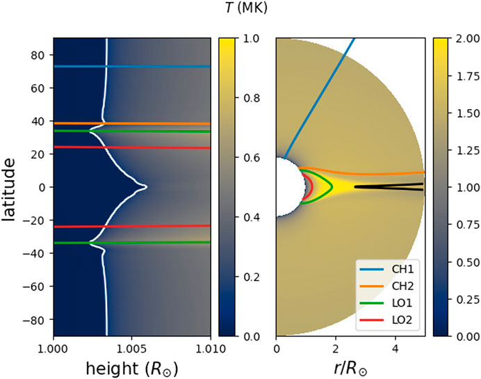
FIGURE 1. Plasma temperature obtained with the global MHD model. On the left panel, we show the temperature profile as a function of latitude and height. The white line shows the contour
The shock capturing ability of PLUTO, based on Riemann solvers, is essential to describe strong density and temperature gradients defining the transition region. Réville et al. (2020b) have developed an additional module to propagate Alfvén waves in the corona. Yet, since this module is based on a Wentzel-Krimers-Brillouin approximation, it is not suited for a precise description of the transition region. To further study the role of turbulence in the composition of the solar wind, we thus rely on the Shell-Atm code, which solves the non-linear incompressible Alfvén wave equations on given profiles along magnetic fields lines, neglecting magneto-acoustic modes. We extracted four different solar wind profiles from our 2.5 D simulation, shown in Figure 1. In the following section, we describe the Shell-Atm simulations made from these profiles.
Shell Turbulence Model
Shell-Atm is a low dimension fluid turbulence code based on the shell technique (see Giuliani and Carbone, 1998; Nigro et al., 2004), that can model coronal loops (Nigro et al., 2004; Buchlin and Velli, 2007) and open solar wind solutions (Verdini et al., 2009). As fixed background profiles of flow speed, density and temperature, we use the four profiles extracted from our global MHD simulation. They are shown in Figure 2. Cases identified with CH correspond to open field regions in Figure 1. The CH1 profile is well in the coronal hole of the northern hemisphere in the fast wind region. CH2 is located close to the streamer and thus in the slow wind region of the simulation. LO cases are coronal loops, the LO1 case being at the open/close boundary with the minimum height of the transition region and LO2 being the smallest loop, well inside the helmet streamer.
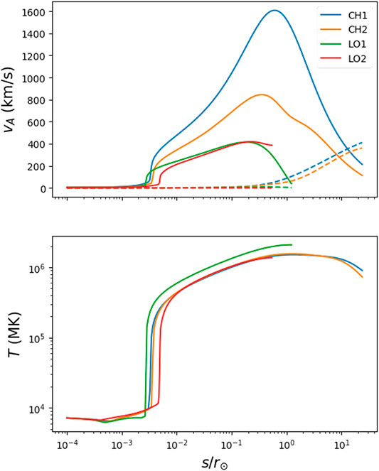
FIGURE 2. Profiles of the Alfvén speed, flow speed (in dashed lines) and temperature for the four field lines extracted from the simulation, along the curvilinear abscissa s. For loops, we only show one side up to the apex. These profiles will be the source of the amplification and reflection (particularly in open regions) of perturbations, the latter leading to the creation of counter-propagating perturbations. Non-linear interactions between counter-propagating waves create the cascade and the dissipation at small scales.
Shell-Atm solves the reduced (incompressible) evolution of Alfvénic fluctuations, i.e. two coupled equations for the evolution of the parallel and anti-parallel wave populations. The transverse components of the fluctuations are discretized in the spectral space, starting from a scale
Transverse motions’ amplitude
We chose to maintain the amplitude
This makes the inner boundary condition partially reflective, with a reflection coefficient being a function of time and of the balance of inward and outward wave populations. Imposing a fully reflecting inner boundary conditions leads indeed to an increase of the base velocity perturbations up to unrealistic values.
Next, we define
the energy flux of the perturbations at any given location in the domain. For both coronal holes and loops cases, we have the total energy injected per second and surface unit at a given time
where the subscripts 0 and 1 denote the bottom and top of the computational domain respectively. In a statistical steady state, we expect to have the losses in the volume compensating for the input energy, i.e.,:
where
is the integrated turbulent heating in the domain and W is the work of the force exerted by the perturbations on the solar wind flow:
The component of the ponderomotive acceleration
where
As we consider one dimensional profile, we use the normalized area
Table 1 sums up all simulations made with the shell model for this work. For each profile geometry, we explore three sets of turbulence parameters referred as cases A, B, and C. In general, we chose the input parameters to create a turbulent heating close to what is observed in the (open) solar wind and as such used in the MHD described in Background Wind and Transition Region Profiles. We find that a transverse perturbation of
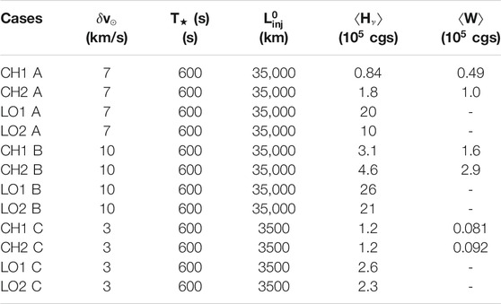
TABLE 1. Parameters and outputs for the Shell-Atm simulations.
In Figure 3, we show some properties of the solutions of the shell model runs A for
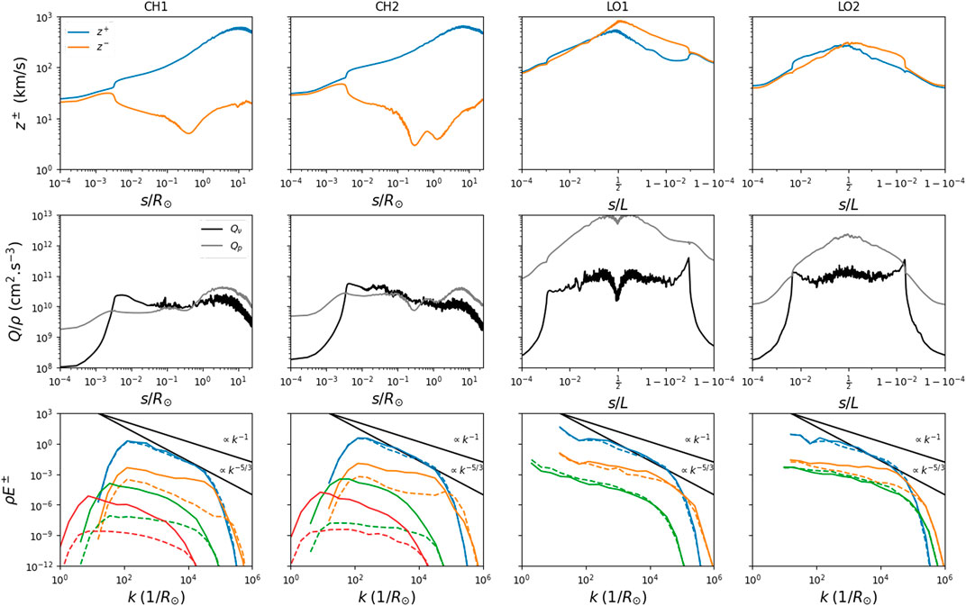
FIGURE 3. Overview of shell simulations A with the same input parameters on the four geometries of coronal holes and loops. The top panel shows the time averaged rms fluctuations
In coronal holes simulations, one striking feature is the regime difference between a mostly balanced turbulence (
As said earlier, the total heating obtained in coronal holes solution
The properties of cases B are very similar to the one of cases A, only with larger wave amplitudes and larger heating rates. For cases C, the wave amplitude is logically smaller, and the cascade extent is also shorter as we remain with a fixed value of the viscosity/resistivity
Ponderomotive Force and First Ionization Potential Fractionation
The main objective of this work is to compare the effect of the turbulence properties on the FIP fractionation for different background configurations. Among the key parameter of the current FIP models is the ponderomotive force, or the wave pressure exerted by the perturbations on the background flow. Figure 4 shows the ponderomotive force obtained in all Table 1 cases, close to the inner boundary, in the chromosphere and transition region. Let us first study the cases A of Table 1, shown in Figure 4 in the top panel. The profile of
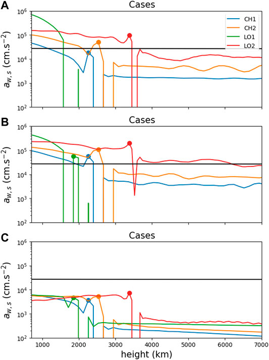
FIGURE 4. Ponderomotive acceleration for all cases of Table 1 in the chromosphere and transition region. Top panel corresponds to cases (A), middle panel to cases (B), with a higher input
For cases B, we observe for the ponderomotive acceleration essentially a shift up of all the curves, conserving the hierarchy of the previous cases as a function of the geometry. For most cases A and B, the strength of the ponderomotive force is higher than the opposing gravity of the Sun, around
We now compute the FIP fractionation created by the ponderomotive force in our models. We use for this the derivation of Laming (2009), that reads:
Here,
where
Figure 5 shows the resulting FIP biases obtained with Eq. 12 and a constant
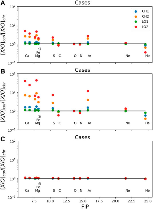
FIGURE 5. FIP biases according to Eq. 12 in the cases (A)(top panel), (B)(middle panel), and (C)(bottom panel) for usual minor ions. The integration is made between
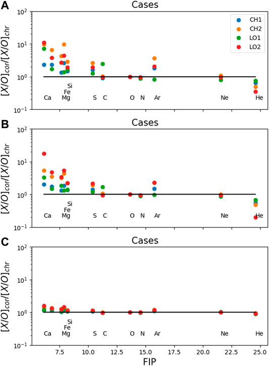
In Figure 6, we repeat the same exercise, but choosing a turbulent velocity
We only sum the shell components for
Discussion
In this work, we have combined several models and tools to assess the efficiency of the Alfvénic turbulence in enriching abundances of low-FIP elements in the low corona. First, we used a global MHD model to get realistic profiles of the Alfvén speed and velocity gradients in both coronal holes and coronal loops, starting from the low chromosphere. They are indeed fundamental in the amplification, reflection and non-linear interaction of propagating Alfvén waves. Then, we took advantage of the Shell-Atm code to compute the interaction between counter-propagating Alfvén waves, the turbulent cascade and the dissipation. Our approach certainly lacks self-consistency, as, for instance, the heating obtained with the shell model is significantly larger in coronal loops than in coronal holes (at least for cases A and B), while the MHD simulation has a much more homogeneous heating. It is, however, the first time that both coronal loops and coronal holes are treated with a shell turbulence model. This model solves the fully non-linear incompressible Alfvén wave equations, including the cascading process and the frequency dependant reflections and interactions of Alfvén wave populations. This is an improvement in comparison with analytical non-WKB approach of previous works (see Laming, 2004; Laming, 2009; Laming, 2012). Moreover, the dissipation is treated physically at very high Lundquist numbers, which cannot be achieved in direct numerical simulations (see, e.g., Dahlburg et al., 2016).
A few comments on the applicability of incompressible MHD to this problem are in order. Reduced MHD equations are derived assuming small gradients in the guide field (or even constant
Wave steepening, shocks and mode conversion, which do create a cascade in the direction parallel to the magnetic field, have typical spectra
Our study shows that, assuming that turbulence is the dominant factor in the coronal heating and solar wind acceleration, a ponderomotive force can appear in the chromosphere and the transition region, and can be strong enough to create a low-FIP bias. This depends however on the turbulence parameters. Injecting energy at the scales of super granules provide the wave amplitude necessary for a low-FIP bias comparable with observations (see, e.g. Feldman, 1992). The force is related to the a amplification of the waves in the corona and the strong gradient that appears at the transition region. Nevertheless, if the energy is injected at the scale of granules, the resulting ponderomotive acceleration seems too weak to explain the observations. Recent works have debated of the right injection scale parameters (van Ballegooijen and Asgari-Targhi, 2017; Chandran and Perez, 2019), and the amplitude of the ponderomotive force could be a way of constraining solar wind turbulence models.
A second result of this study is that the low-FIP bias is not exclusive to coronal loops. Interestingly, we obtain significant low-FIP bias for open field configurations along the streamer (CH2). We also have usually little FIP bias for the LO1 loop, i.e., the loop at the very edge of the helmet streamer. This result might seem in opposition with previous works, such as the one of Laming (2004), Laming (2015). Their result is indeed the consequence of resonant Alfvén waves in the loops, likely triggered by reconnection, which amplify significantly the ponderomotive acceleration. Injecting transverse motions from the inner boundary, we do not observe such resonances, and further studies are needed to compare the relative importance of different triggers. We do show however that resonances are not needed to obtain a low-FIP bias in coronal loops and open slow wind regions. This study thus questions, anyhow, the necessity of interchange reconnection to explain the composition of the slow solar wind.
Finally, it is important to stress that our modeling of the solar chromosphere is very simple. We assume, following Laming (2004), Laming (2009) and writing Eq. 12, that proton drag, collisions and turbulent mixing, are exactly compensating for the Sun’s gravity pull in the chromosphere. The actual balance of all these processes remains very hard to estimate. Shocks and compressible fluctuations are also believed to be significant in the chromosphere and even in the transition region (see Carlsson et al., 2019, for a recent review) and are not accounted for in the shell simulations. Ongoing works are dedicated to build a compressible kinetic-fluid model, including heavy ions populations with various charge state and their interactions with protons and waves.
Data Availability Statement
The raw data supporting the conclusions of this article will be made available by the authors, without undue reservation.
Author Contributions
VR is the main developer of the multi-D MHD model and performed all simulations. AV, ÉB, and MV are the main developers of the SHELL-ATM code. All authors have contributed to the data analysis, text editing and discussions.
Funding
This research was funded by the ERC SLOW SOURCE project (SLOW SOURCE–DLV-819189). MV was supported by the NASA HERMES Drive Science Center grant No. 80NSSC20K0604. We thank M. Laming for very useful discussions. Numerical computations were performed using GENCI grants numbers A0080410133 and A0070410293. This study has made use of the NASA Astrophysics Data System.
Conflict of Interest
The authors declare that the research was conducted in the absence of any commercial or financial relationships that could be construed as a potential conflict of interest.
References
Alazraki, G., and Couturier, P. (1971). Solar wind accejeration caused by the gradient of alfven wave pressure. Astron. Astrophys. 13, 380–389.
Antiochos, S. K., Linker, J. A., Lionello, R., Mikić, Z., Titov, V., and Zurbuchen, T. H. (2012). The structure and dynamics of the corona-heliosphere connection. Space Sci. Rev. 172, 169–185. doi:10.1007/s11214-011-9795-7
Belcher, J. W. (1971). Alfvénic wave pressures and the solar wind. Astrophys. J. 168, 509. doi:10.1086/151105
Belcher, J. W., and Davis, L. (1971). Large-amplitude Alfvén waves in the interplanetary medium, 2. J. Geophys. Res. 76 (16), 3534–3563. doi:10.1029/ja076i016p03534
Bochsler, P., Geiss, J., and Kunz, S. (1986). Abundances of carbon, oxygen, and neon in the solar wind during the period from August 1978 to June 1982. Sol. Phys. 103 (1), 177–201. doi:10.1007/bf00154867
Bruno, R., and Carbone, V. (2013). The Solar wind as a turbulence laboratory. Living Rev. Sol. Phys. 10, 2. doi:10.12942/lrsp-2013-2
Buchlin, E., and Velli, M. (2007). Shell models of RMHD turbulence and the heating of solar coronal loops. Astrophys. J. 662 (1), 701–714. doi:10.1086/512765
Carlsson, M., De Pontieu, B., and Hansteen, V. H. (2019). New view of the solar chromosphere. Annu. Rev. Astron. Astrophys. 57 (1), 189–226. doi:10.1146/annurev-astro-081817-052044
Chandran, B. D. G., and Hollweg, J. V. (2009). Alfvén wave reflection and turbulent heating in the solar wind from 1 solar radius to 1 Au: an analytical treatment. Astrophys. J. 707 (2), 1659–1667. doi:10.1088/0004-637x/707/2/1659
Chandran, B. D. G., and Perez, J. C. (2019). Reflection-driven magnetohydrodynamic turbulence in the solar atmosphere and solar wind. J. Plasma Phys. 85 (4), 905850409. doi:10.1017/s0022377819000540
Dahlburg, R. B., Laming, J. M., Taylor, B. D., and Obenschain, K. (2016). Ponderomotive acceleration in coronal loops. Astrophys. J. 831 (2), 160. doi:10.3847/0004-637x/831/2/160
Dere, K. P., Landi, E., Mason, H. E., Monsignori Fossi, B. C., and Young, P. R. (1997). CHIANTI—an atomic database for emission lines. Astron. Astrophys. Suppl. Ser. 125 (1), 149–173. doi:10.1051/aas:1997368
DeRosa, M. L., Brun, A. S., and Hoeksema, J. T. (2012). Solar magnetic field reversals and the role of dynamo families. Astrophys. J. 757 (1), 96. doi:10.1088/0004-637x/757/1/96
Dmitruk, P., Matthaeus, W. H., Milano, L. J., Oughton, S., Zank, G. P., and Mullan, D. J. (2002). Coronal heating distribution due to low‐frequency, wave‐driven turbulence. Astrophys. J. 575 (1), 571–577. doi:10.1086/341188
Feldman, U. (1992). Elemental abundances in the upper solar atmosphere. Phys. Scripta 46 (3), 202–220. doi:10.1088/0031-8949/46/3/002
Geiss, J., Gloeckler, G., and von Steiger, R. (1995). Origin of the solar wind from composition Data. Space Sci. Rev. 72 (1–2), 49–60. doi:10.1007/978-94-011-0167-7_8
Giuliani, P., and Carbone, V. (1998). A note on shell models for MHD Turbulence. Europhys. Lett. 43 (5), 527–532. doi:10.1209/epl/i1998-00386-y
Gloeckler, G., and Geiss, J. (1989). The abundances of elements and isotopes in the solar wind. AIP Conf. Proc. 183 (1), 49–71. doi:10.1063/1.37985
Jacques, S. A. (1977). Momentum and energy transport by waves in the solar atmosphere and solar wind. Astrophys. J. 215, 942. doi:10.1086/155430
Laming, J. M. (2004). A unified picture of the first ionization potential and inverse first ionization potential effects. Astrophys. J. 614 (2), 1063–1072. doi:10.1086/423780
Laming, J. M. (2009). Non-WKB models of the first ionization potential effect: implications for solar coronal heating and the coronal helium and neon abundances. Astrophys. J. 695 (2), 954–969. doi:10.1088/0004-637x/695/2/954
Laming, J. M. (2012). Non-WKB models of the first ionization potential effect: the role of slow mode waves. Astrophys. J. 744 (2), 115. doi:10.1088/0004-637x/744/2/115
Laming, J. M. (2015). The FIP and Inverse FIP Effects in Solar and Stellar Coronae. Living Rev. Sol. Phys. 12, 2. doi:10.1007/lrsp-2015-2
Leer, E., Holzer, T. E., and Flå, T. (1982). Acceleration of the solar wind. Space Sci. Rev. 33, 161–200. doi:10.1007/BF00213253
Lionello, R., Linker, J. A., and Mikić, Z. (2001). Including the transition region in models of the large‐scale solar corona. Astrophys. J. 546 (1), 542–551. doi:10.1086/318254
Litwin, C., and Rosner, R. (1998). Coronal scale-height enhancement by magnetohydrodynamic waves. Astrophys. J. 506 (2), L143–L146. doi:10.1086/311656
Marsch, E., von Steiger, R., and Bochsler, P. (1995). Element fractionation by diffusion in the solar chromosphere. Astron. Astrophys. 301, 261–276.
Meyer, J.-P. (1985a). The baseline composition of solar energetic particles. Astrophys. J. Suppl. Ser. 57, 173–204.
Meyer, J.-P. (1985b). The baseline composition of solar energetic particles. Astrophys. J. Suppl. Ser. 57, 151–171. doi:10.1086/191000
Mignone, A., Bodo, G., Massaglia, S., Matsakos, T., Tesileanu, O., Zanni, C., et al. (2007). PLUTO: a numerical code for computational Astrophysics. Astrophys. J. Suppl. Ser. 170 (1), 228–242. doi:10.1086/513316
Nakariakov, V. M., and Verwichte, E. (2005). Coronal Waves and Oscillations. Living Rev. Sol. Phys. 2, 3. doi:10.12942/lrsp-2005-3
Nigro, G., Malara, F., Carbone, V., and Veltri, P. (2004). Nanoflares and MHD turbulence in coronal loops: a hybrid shell model. Phys. Rev. Lett. 92 (19), 194501. doi:10.1103/physrevlett.92.194501
Oughton, S., Matthaeus, W. H., and Dmitruk, P. (2017). Reduced MHD in astrophysical applications: two-dimensional or three-dimensional? Astrophys. J. 839 (1), 2. doi:10.3847/1538-4357/aa67e2
Perez, J. C., and Chandran, B. D. G. (2013). Direct numerical simulations of reflection-driven, reduced magnetohydrodynamic turbulence from the Sun to the Alfvén critical point. Astrophys. J. 776 (2), 124. doi:10.1088/0004-637x/776/2/124
Réville, V., Tenerani, A., and Velli, M. (2018). Parametric decay and the origin of the low-frequency alfvénic spectrum of the solar wind. Astrophys. J. 866 (1), 38. doi:10.3847/1538-4357/aadb8f
Réville, V., Velli, M., Panasenco, O., Tenerani, A., Shi, C., Badman, S. T., et al. (2020a). The role of Alfvén wave dynamics on the large-scale properties of the solar wind: comparing an MHD simulation with parker solar probe E1 Data. Astrophy. J. Suppl. Ser. 246 (2), 24. doi:10.3847/1538-4365/ab4fef
Réville, V., Velli, M., Rouillard, A. P., Lavraud, B., Tenerani, A., Shi, C., et al. (2020b). Tearing instability and periodic density perturbations in the slow solar wind. Astrophy. J. Suppl. Ser. 895 (1), L20. doi:10.3847/2041-8213/ab911d
Saha, M. N. (1920). Ionisation in the solar chromosphere. Nature 105 (2634), 232–233. doi:10.1038/105232b0
Saha, M. N. (1921). On a physical theory of stellar spectra. Proc. Royal Soc. London Ser. A 99, 135–153. doi:10.1098/rspa.1921.0029
Schwadron, N. A., Fisk, L. A., and Zurbuchen, T. H. (1999). Elemental fractionation in the slow solar wind. Astrophy. J. 521 (2), 859–867. doi:10.1086/307575
Shoda, M., Suzuki, T. K., Asgari-Targhi, M., and Yokoyama, T. (2019). Three-dimensional simulation of the fast solar wind driven by compressible magnetohydrodynamic turbulence. Astrophy. J. 880 (1), L2. doi:10.3847/2041-8213/ab2b45
Shoda, M., Yokoyama, T., and Suzuki, T. K. (2018a). A self-consistent model of the coronal heating and solar wind acceleration including compressible and incompressible heating processes. Astrophy. J. 853 (2), 190. doi:10.3847/1538-4357/aaa3e1
Shoda, M., Yokoyama, T., and Suzuki, T. K. (2018b). Frequency-dependent Alfvén-wave propagation in the solar wind: onset and suppression of parametric decay instability. Astrophy. J. 860 (1), 17. doi:10.3847/1538-4357/aac218
Strauss, H. R. (1976). Nonlinear, three-dimensional magnetohydrodynamics of noncircular tokamaks. Phys. Fluids 19 (1), 134. doi:10.1063/1.861310
Tenerani, A., and Velli, M. (2013). Parametric decay of radial Alfvén waves in the expanding accelerating solar wind. J. Geophys. Res. Space Phys. 118 (12), 7507–7516. doi:10.1002/2013ja019293
Tu, C.-Y., and Marsch, E. (1995). MHD structures, waves and turbulence in the solar wind: observations and theories. Space Sci. Rev. 73, 1–210. doi:10.1007/BF00748891
van Ballegooijen, A. A., and Asgari-Targhi, M. (2017). Direct and inverse cascades in the acceleration region of the fast solar wind. Astrophys. J. 835 (1), 10. doi:10.3847/1538-4357/835/1/10
van Ballegooijen, A. A., Asgari-Targhi, M., Cranmer, S. R., and DeLuca, E. E. (2011). Heating of the solar chromosphere and corona by Alfvén wave turbulence. Astrophy. J. 736 (1), 3. doi:10.1088/0004-637x/736/1/3
van Ballegooijen, A. A., and Asgari-Targhi, M. (2016). Heating and acceleration of the fast solar wind by Alfvén wave turbulence. Astrophy. J. 821 (2), 106. doi:10.3847/0004-637x/821/2/106
Velli, M., Grappin, R., and Mangeney, A. (1989). Turbulent cascade of incompressible unidirectional Alfvén waves in the interplanetary medium. Phys. Rev. Lett. 63 (17), 1807–1810. doi:10.1103/physrevlett.63.1807
Verdini, A., Grappin, R., and Montagud-Camps, V. (2019). Turbulent Heating in the Accelerating Region Using a Multishell Model. Solar Phy. 294, 65. doi:10.1007/s11207-019-1458-y
Verdini, A., and Velli, M. (2007). Alfvén waves and turbulence in the solar atmosphere and solar wind. Astrophy. J. 662 (1), 669–676. doi:10.1086/510710
Verdini, A., Velli, M., and Buchlin, E. (2009). Turbulence in the sub-alfvénic solar wind driven by reflection of low-frequency Alfvén waves. Astrophy. J. 700 (1), L39–L42. doi:10.1088/0004-637x/700/1/l39
Wood, B. E., and Linsky, J. L. (2010). Resolving the ξ BOO binary withchandra, and revealing the spectral type dependence OF the coronal “FIP effect”. Astrophy. J. 717 (2), 1279–1290. doi:10.1088/0004-637x/717/2/1279
Zank, G. P., and Matthaeus, W. H. (1992). The equations of reduced magnetohydrodynamics. J. Plasma Phys. 48 (1), 85–100. doi:10.1017/s002237780001638x
Zank, G. P., and Matthaeus, W. H. (1993). Nearly incompressible fluids. II: magnetohydrodynamics, turbulence, and waves. Phys. Fluid. Fluid Dynam. 5 (1), 257–273. doi:10.1063/1.858780
Keywords: turbulence, slow wind, transition region, chromosphere, Alfvén waves
Citation: Réville V, Rouillard AP, Velli M, Verdini A, Buchlin É, Lavarra M and Poirier N (2021) Investigating the Origin of the First Ionization Potential Effect With a Shell Turbulence Model. Front. Astron. Space Sci. 8:619463. doi: 10.3389/fspas.2021.619463
Received: 20 October 2020; Accepted: 04 January 2021;
Published: 08 February 2021.
Edited by:
Luca Sorriso-Valvo, Institute for Space Physics, SwedenReviewed by:
Mahboubeh Asgari-Targhi, Harvard University, United StatesGiuseppina Nigro, Università Della Calabria, Italy
Copyright © 2021 Réville, Rouillard, Velli, Verdini, Buchlin, Lavarra and Poirier. This is an open-access article distributed under the terms of the Creative Commons Attribution License (CC BY). The use, distribution or reproduction in other forums is permitted, provided the original author(s) and the copyright owner(s) are credited and that the original publication in this journal is cited, in accordance with accepted academic practice. No use, distribution or reproduction is permitted which does not comply with these terms.
*Correspondence: Victor Réville, dmljdG9yLnJldmlsbGVAaXJhcC5vbXAuZXU=