Velocity Distribution Associated With EUV Disturbances Caused by Eruptive MFR

Extreme ultraviolet (EUV) disturbances are ubiquitous during eruptive phenomena like solar flare and Coronal Mass Ejection (CME). In this work, we have performed a three-dimensional (3D) magnetohydrodynamic numerical simulation of CME with an analytic magnetic fluxrope (MFR) to study the complex velocity distribution associated with EUV disturbances. When the MFR erupts upward, a fast shock (FS) appears as a 3D dome, followed by outward moving plasma. In the center of the eruptive source region, an expanding CME bubble and a current sheet continuously grow, both of which are filled by inward moving plasma. At the flanks of the CME bubble, a complex velocity distribution forms because of the dynamical interaction between inward and outward plasma, leading to the formation of slow shock (SS) and velocity separatrix (VS). We note two types of vortices near the VS, not mentioned in the preceding EUV disturbance simulations. In first type of vortex, the plasma converges toward the vortex center, and in the second type, the plasma spreads out from the center. The forward modeling method has been used to create the synthetic SDO/AIA images, in which the eruptive MFR and the FS appear as bright structures. Furthermore, we also deduce the plasma velocity field by utilizing the Fourier local correlation tracking method on the synthetic images. However, we do not observe the VS, the SS, and the two types of vortices in this deduced velocity field.

1 Introduction

Coronal disturbances in extreme ultraviolet (EUV), soft X-ray (SXR), and other wavebands during the solar flare and coronal mass ejection (CME) eruptive events have been observed and simulated extensively during past decades (Liu and Ofman, 2014; Warmuth, 2015). To understand their observed characteristics, the researchers proposed three kind of models based on numerical simulation studies, i. e., magnetohydrodynamic (MHD) wave/shock models (Uchida, 1970; Vršnak and Cliver, 2008; Selwa et al., 2012; Wang et al., 2021), non-wave models (Chen et al., 2002; Attrill et al., 2007; Delannée et al., 2008) and hybrid models (Chen et al., 2005; Cohen et al., 2009; Downs et al., 2012; Mei et al., 2020a; Mei et al., 2020b; Downs et al., 2021). The wave models explain the EUV disturbances as fast MHD shock during the flare/CME events. This wave interpretation is supported by lots of observations, including reflection, refraction and transmission across magnetic structures (Thompson and Myers, 2009; Shen and Liu, 2012; Kienreich et al., 2013; Shen et al., 2013; Muhr et al., 2014), broadening of shock front and its decreased amplitude (Wills-Davey et al., 2007; Muhr et al., 2011; Long et al., 2017) and quasi-periodic wave trains (Liu et al., 2011; Liu et al., 2012; Nisticò et al., 2014; Zheng et al., 2018; Shen et al., 2019). In non-wave models, the EUV disturbances were explained as adjusting of the magnetic field due to the expanding CME bubble. In the high-cadence AIA observations, researchers report lots of events with both wave and non-wave disturbances (Liu et al., 2010; Chen and Wu, 2011; Asai et al., 2012; Cheng et al., 2012; Liu et al., 2013; Cunha-Silva et al., 2018; Fulara et al., 2019). The bimodality characteristics of coronal disturbances support the hybrid models. In a typical physical scene of the hybrid model, a fast shock for the wave component of the disturbance appears in front of the upward erupting CME, the CME bubble (Downs et al., 2012) or other accompanied structures, such as helical current boundary/current shell (Delannée et al., 2008; Mei et al., 2020a) are responsible for the non-wave component.

Although the hybrid models have become widely accepted by researchers, there exist some remain problems. For example, in the numerical simulation of EUV disturbances, some physical processes, such as vortices, slow MHD shock wave (SS), and velocity separatrix (VS), has been noticed and should exist as ubiquitous as the fast MHD wave/shock in realistic observations. However, they have not been confirmed by observational studies. Forbes (1990) had shown the vortices on both sides of the CME in a 2D MHD simulation, which has also been confirmed by Wang et al. (2009) and Mei et al. (2012). Wang et al. (2009) had performed a 2D simulation and proposed the SS as one of the physical mechanisms behind coronal disturbances. Furthermore, Mei et al. (2020b) had performed 3D MHD simulation for EUV disturbance and find that the SS is associated with a VS, which separates plasma moving inward to the center of the eruptive source region and plasma moving after the fast shock (FS). These numerical simulations reflect the existence of a velocity distribution with complex structure in the eruptive source region, which results from the interaction among the CME, the FS and other structures. In this work, we utilize the Titov and Démoulin (1999) model (TD99 hereafter) to perform a 3D high-resolution MHD numerical simulation of the eruptive MFR, emphasizing the complex velocity field and corresponding EUV manifestations. Here, we use the forward modeling method (Van Doorsselaere et al., 2016) to create the synthetic SDO/AIA images to directly compare our numerical results with actual observations. In the studies of EUV disturbances and other phenomena during the eruption, the synthetic images method has been widely used to compare the numerical models with the actual observations, such as X-ray sigmoids (Roussev et al., 2012), prominence formation (Xia and Keppens, 2016), the global EUV disturbances (Downs et al., 2012, 2021; Mei et al., 2020a; Mei et al., 2020b), the CME and reconnecting current sheet in EUV emission (Lugaz et al., 2011; Pagano et al., 2014; Zhao et al., 2019; Ye et al., 2020) and white-light (Lugaz et al., 2007; Manchester et al., 2008; Jin et al., 2017). Furthermore, the Fourier local correlation tracking code (Fisher and Welsch, 2008; Fisher and Welsch, 2020) has been applied to the synthetic images to deduce the velocity field, in which the vortices, the SS, and the VS may appear. In Section 2, the setup of this simulation is given; in Section 3, the main results are presented; in the last section, we summarize this work.

2 Setup of Simulation

Utilizing the MPI-parallelized adaptive mesh refinement code (MPI-AMRVAC) (Keppens et al., 2012; Porth et al., 2014; Xia et al., 2018; Keppens et al., 2020), this simulation’s governing resistive MHD equations are solved numerically by a three-order accurate finite volume scheme, which consists of a Harten-Lax-van Leer approximate Riemann solver (Harten, 1983), a third-order slope limiter (Čada and Torrilhon, 2009) and a three-step Runge–Kutta time-marching method. The simulation domain is a box of size −6 ≤ x ≤ 6, −6 ≤ y ≤ 6, and 0 ≤ z ≤ 12 in the Cartesian coordinate system, which resolves by 360³ uniformly distributed grid points. The dimensionless units for length, velocity, pressure, and magnetic field are 5 × 10⁹ cm, 1.2 × 10⁷ cm s⁻¹, 3.2 Pa and 6.3 G respectively.

The initial magnetic structure comes from the well-known TD99 model, which consists of an MFR to model filament/prominence, a background field to confine the MFR, and a dipole to control the twist feature of the MFR (see Figure 1 in Mei et al., 2020b). The MFR has been described by parameters major radius R, minor radius a, and total toroidal current I along the MFR axis. The background field comes from a pair of magnetic sources ± q separated by a distance L, lying on the MFR symmetry axis. The dipole introduces an extra toroidal component around the MFR to control the twist profile of the MFR. Although the analytical model is much simpler than a realistic magnetic structure, this simple model allows us to study the fundamental physical process during MFR eruption without being disturbed by other features. On the other hand, we have adopted gravity stratification atmosphere and thermal conduction, two crucial components for obtaining reliable density and temperature distributions during the MFR eruption and creating synthetic EUV image. The heat conduction aligns the magnetic field line, hence $\kappa ={\kappa }_{\parallel }{T}^{2/5}{\widehat{e}}_B{\widehat{e}}_B$, with ${\widehat{e}}_B=\vec{B}/|B|$ and κ_∥ = 10^–6 erg s⁻¹ cm⁻¹ K^−3.5. The super-time-stepping scheme has been used to handle the heat conduction term to significantly reduce iterations and improve stability when the plasma temperature exceeds10⁷ K (Alexiades et al., 1996; Meyer et al., 2012; Zhou et al., 2021).

FIGURE 1

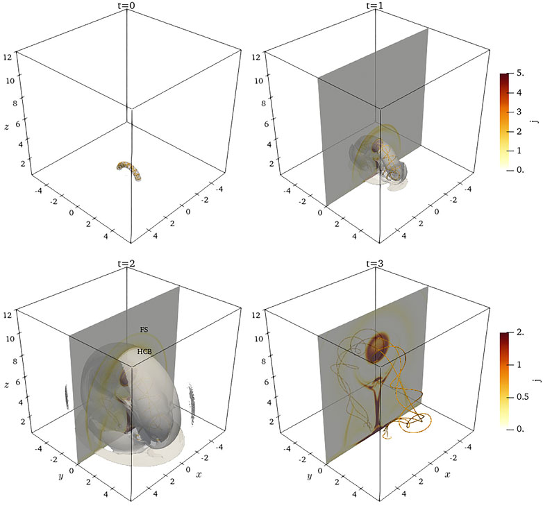
FIGURE 1. Evolution snapshots of eruptive magnetic fluxrope (MFR) at different times. The units of time and length are 4.3 × 102 s and 5 × 10⁹ cm. The golden curves are magnetic field lines of the MFR. The distribution of electric current is on the cut y = 0, which shows the upward moving of the MFR and the resultant formation of the current sheet (CS), the fast shock (FS), the slow shock (SS), and the helical current boundary (HCB).

We use a two-layer gravitationally stratified atmosphere, with z ≤ z_p and z > z_p representing the photosphere and the corona, respectively. Here, the photosphere provides a high-beta environment to realize a line-tied bottom boundary, where the magnetic field line foot-points are anchored into photosphere (Wang et al., 2009; Mei et al., 2012; Wang et al., 2015; Xie et al., 2019). At the height z = z_p, the plasma pressure equals 0.2 Pa, the strength of the magnetic field nearby the MFR can reach 100 G, and so the plasma beta value approximately equals 10^–4, which is close to the realistic coronal environment. In addition, for the other five boundaries, we adopt the simplest open boundary conditions, i.e., all physical quantities are deduced via the extrapolation of internal grid points. Detail formulae of components of magnetic structure and two-layer stratified atmosphere had been already given in Mei et al. (2020b). Involved parameters for initial magnetic configuration and atmosphere are the same with Mei et al. (2020a), and one can refer to this work for more detail.

3 Numerical Results

The MFR starts to erupt immediately after the simulation begins because of the un-equilibrium initial magnetic structure and so a net upward Lorenz force acting on the initial MFR. In the meanwhile, the MFR experiences kink instabilities due to the high twist turn of the MFR. Figure 1 shows the evolution snapshots of the eruptive MFR. The golden twisted curves are magnetic field lines inside the MFR, which show significant expansion during the eruption. The electric current distribution on a plane y = 0 shows that several structures appear as a result of the upward rise of the MFR, including the FS, the helical current boundary (HCB) and other features. The FS is a piston-driven shock invoked by the MFR (Wang et al., 2009), which means that its outward moving speed can be much faster than the MFR, as shown in Figure 1. The HCB results from the interaction between the background magnetic field and the upward eruptive magnetic structure. Its helical shape comes from the rotation movement of the MFR because of the kink instability. After a short acceleration process in the very early stage, the MFR, the HCB, and the FS expand outward with almost constant speeds of 360 km s⁻¹, 470 km s⁻¹ and 500 km s⁻¹ respectively. These kinetic features of the eruptive magnetic structure have been significantly affected by the magnetic reconnection rate and fine structure inside a 3D current sheet (CS) (Mei et al., 2017), which grows continuously under the MFR.

The distribution of density ρ, temperature T and velocity curl $\nabla \times \vec{v}$ on cut x = 0 and z = z_p (low-left panel) at t = 2 are shown in Figure 2. The grey arrows show the velocity distribution, and its length has been scaled by the norm of velocity vector $|\vec{v}|$. For the cut x = 0, the velocity distribution shows that parts of plasma move toward the reconnecting CS and the CME bubble, and part of plasma moves outward, following the FS. Between two streams of plasma, there exists a VS marked by a pink curve. The top-tip of this curve connects to a vortex region, which is already noticed by preceding 2D numerical simulations (Forbes, 1990; Wang et al., 2009). For the cut z = z_p, the grey isosurface $|\vec{v}|=0.07$ approximately illustrates the position of the 3D VS. Inside the VS, plasma moves toward the center of the eruptive source region. Outside the VS, plasma follows the expanding FS front. In addition, around the VS, there exists a SS, as indicated by colorful shading of velocity curl.

FIGURE 2

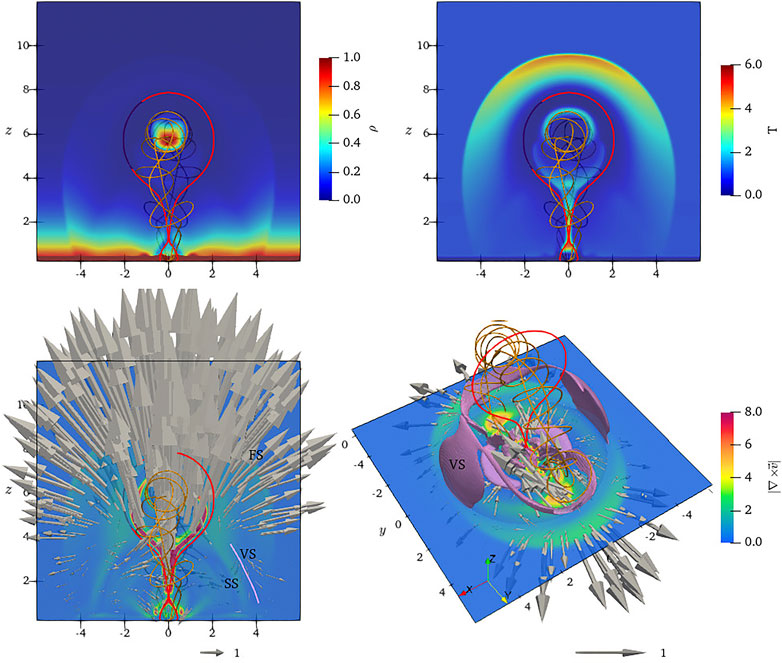
FIGURE 2. Distributions (coloured shading) of density ρ, temperature T and velocity curl $\nabla \times \vec{v}$ and distribution (3D yellow arrows) of velocity on cuts y = 0 and z = z_p at t = 2. The fast shock (FS), the slow shock (SS), and the velocity separatrix (VS) are marked on the panels. The golden and red curves are magnetic field lines of the MFR and the outer boundary of the CME bubble. The pink isosurface |v| = 0.07 illustrates the 3D VS approximately.

The structure of the velocity field at t = 3 is also shown by eight groups of streamlines in Figure 3. In all panels, the golden and red curves are magnetic field lines of the MFR and the outer boundary of the CME bubble, respectively. In the upper panels, the streamlines (light-green and light-purple curves) illustrate the velocity field structures in quadrants II and IV of the x-y coordinate system. The light-green streamlines show plasma flow related to the reconnection inflow and the CME bubble. They originate from regions R1 marked in the upper-left panel, located in the lower atmosphere near the foot-points of the MFR. The plasma in R1 comes to the side of the 3D CS through a vortex channel surrounding the MFR. Later, it enters into the CS as reconnection inflow and finally becomes parts of the CME bubble or flare loop system. Unlike light-green curves, the light-purple curves illustrate another kind of plasma stream, only related to the FS. It originates from region R2, located at the bottom of the simulation box. It indicates a stream of plasma moves upward and follows the expanding FS. In the lower panels, the streamlines show plasma flow structures in the I and III quadrants. Like the curves in upper panels, the green streamlines relate to the reconnection inflow and CME bubble, and the purple ones are associated with the FS. However, unlike the curves in upper panels, the green and purple streamlines originate from the same region R3, marked on the lower-left panel.

FIGURE 3

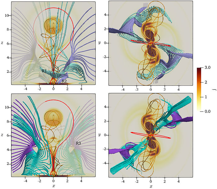
FIGURE 3. Several groups of velocity streamlines (colorful curves) show complex plasma flow field structures around the CME at t = 3. Golden curves are the magnetic field line of the MFR; Red curves give the CME bubble boundary (Upper row) The light-green and light-purple curves are velocity streamlines in quadrants II and IV of the x-y coordinate system. (Lower row) The green and purple curves are velocity streamlines in quadrants I and III.

Furthermore, the relationship among streamlines, the VS, and the vortexes are presented in panel (a) of Figure 4. The streamlines in quadrants I and II are the same with the curves in upper panel of Figure 3. The grey iso-surfaces with $\left|v\right|=0.07$ illustrate the location of the 3D VS in the lower atmosphere of the eruptive source region. These streamlines show that the plasma inside the VS moves inward to the CS and the CME bubble, and the plasma outside moves outward. The regions R1, R2 and R3 are nearby the VS. Two grey slices inside two boxes have been chosen, as marked in panel (a), to illustrate the detailed information of velocity distribution nearby these regions. Panels (b) and (c) have given velocity fields on these two slices.

FIGURE 4

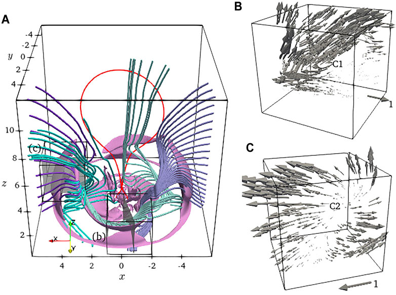
FIGURE 4. (A)Velocity streamlines in quadrants I (green and purple) and II (light-green and light-purple) of the x-y coordinate system at t = 3. The pink surfaces are velocity iso-surfaces with $\left|\vec{v}\right|=0.07$, which indicates the location of the VS. The red curve shows the CME bubble boundary. (B) and (C)Velocity fields on grey cuts inside two boxes, which show two types of vortexes.

In panel (b), we can see a vortex center labeled as C1. The surrounding velocity field arrows show that ambient plasma moves around, converges toward C1, and finally forms a vortex channel, as already demonstrated by the colorful streamlines. This vortex channel transports the plasma near the region R1 and R2 to the ambient region around the reconnection CS and the CME bubble. Part of the transported plasma moves toward the FS, and others move toward the CS and the CME bubble, contributing to the plasma composition of the CME bubble. Although we have not considered the composition and ionization state of the plasma in this work, a more realistic numerical experiment likely also exists in the vortex channel. This transport process suggests that the plasma composition at the lower atmosphere can change the plasma composition inside the CME bubble.

In panel (c), another type of vortex center is labeled as C2, that all velocity arrows rotate around and spread away from it. Also, part of the plasma moves toward the FS, and others move toward the CS and the CME bubble. Unlike C1, no vortex channels associated with C2 can be seen. Because of the slight streamline distortion at the vortex center and the low plasma beta, a noticeable vortex channel can not form, and so there is no continual plasma that has been transported into the vortex center to compensate for scattered plasma away from the center.

In Figure 5, the synthetic SDO/AIA 193Å, 171Å and 131Å images are shown to give observational features of our numerical results. These images are created by utilizing the forward modeling code FOMO (Van Doorsselaere et al., 2016), which translate the plasma density and temperature of the optically thin coronal atmosphere in numerical simulation into the EUV emission and then integrated along the line-of-sight (LOS). The coordination system of our numerical simulation connects to the rotated frame-of-reference of the observer by two angles $\mathcal{L}$ and $\mathcal{B}$. Here, $\mathcal{L}$ is between the LOS and the z-axis, $-\mathcal{B}$ is between the LOS and the y-axis. The synthetic images plane (i.e., the plane-of-the-sky, POS) is perpendicular to the LOS. In the beginning, the MFR appears as a dark filament because of the low temperature of its internal plasma. At t = 1, the MFR has been brightened due to its internal untwisting process and resultant magnetic reconnection. The FS front can be seen clearly as a 3D bright dome. Later, the MFR expands outward adiabatic, and so its brightness decays continuously. Due to the different contribution functions for 171Å and 131Å (Lemen et al., 2012), the MFR and the FS in the lower panels are slightly different from the upper panels. At t = 2, the HCB can been seen in the 171Å and 131Å images. Different from the FS, the HCB should be classified as non-wave components of the EUV disturbance.

FIGURE 5

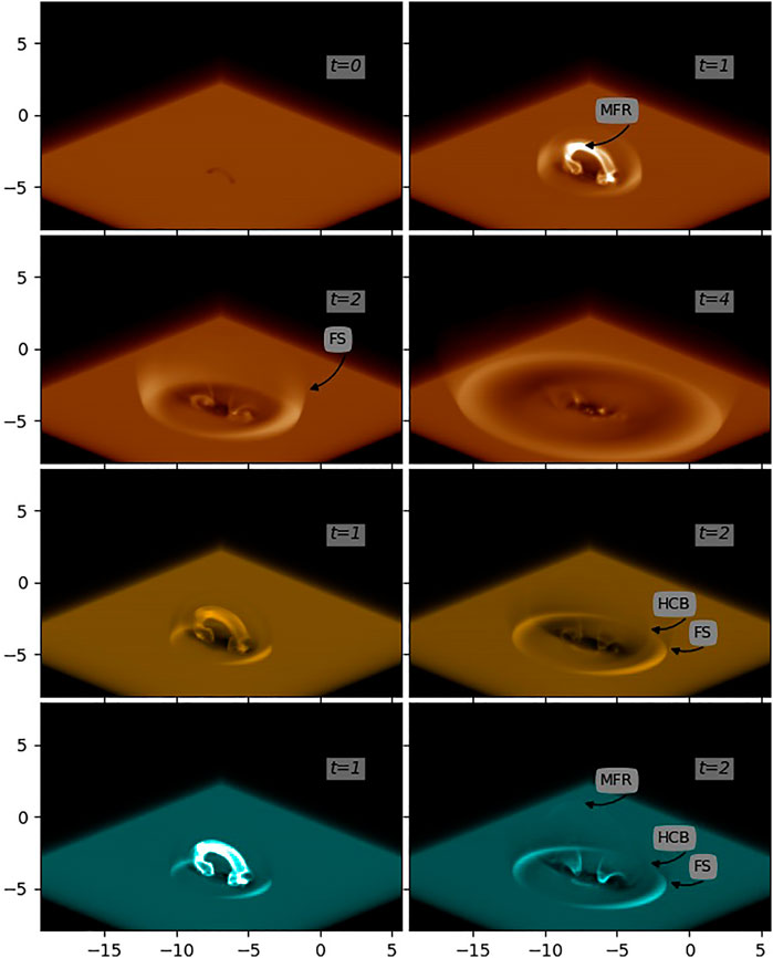
FIGURE 5. Synthetic images of AIA 193Å (upper two lows), 171Å (third low) and 131Å (bottom low) in the plane-of-the-sky (POS) with view angles $\mathcal{L}=-45°$ and $\mathcal{B}=60°$ at different times.

The velocity field is very important to diagnose the nature of the EUV disturbance. It is valuable to determine whether we can deduce a reliable plasma velocity distribution from the realistic EUV observations, and whether these deduced velocity field are similar to these shown in Figure 2. Therefore, we utilize the Fourier local correlation tracking code FLCT (Fisher and Welsch, 2008; Fisher and Welsch, 2020) to deduce velocity field. The FLCT estimates a 2D velocity field from two successive images. The first image evolves into the second image over a small time step, which usually depends on observations’ time resolution. Instead to apply the FLCT to realistic observations, here we apply them to our synthetic images with different view angles at t = 2, 2 + Δt, four and 4 + Δt. Here, Δt = 0.0023 times the dimensionless unit of time equals one second. Figure 6 show the synthetic images of AIA 193Å with log-scale. In all panels, black arrows show the deduced velocity fields. In the top panels of Figure 6, the synthetic image shows a situation in which the EUV disturbance has been observed in the limb. The velocity field inside the two boxes marked on the top panels is shown in the middle panels. Unfortunately, the deduced velocity does not consist of inward plasma flow and outward flow, significantly different from the velocity distribution on cut x = 0 in Figure 2. In the bottom panels of Figure 6, the EUV disturbance has been observed on the solar disk. The black arrows show that almost all plasma move outward to the expanding FS front, which is also different from the velocity field on cut z = z_p, shown in Figure 2. The apparent difference between the deduced velocity field and the velocity field shown in Figure 2 comes from the fact that the deduced velocity is based on the EUV emission and involves an integration along the LOS. In the deduced images, we can not see the VS, the SS and the vortex, so that explains why they have not been reported usually in realistic observations, although the numerical simulation indicates that they should present similar to the ubiquitous FS. In other words, applying FLCT on realistic AIA images, the deduced velocity field can not provide essential evidence for the existence of the VS, the SS and the vortex.

FIGURE 6

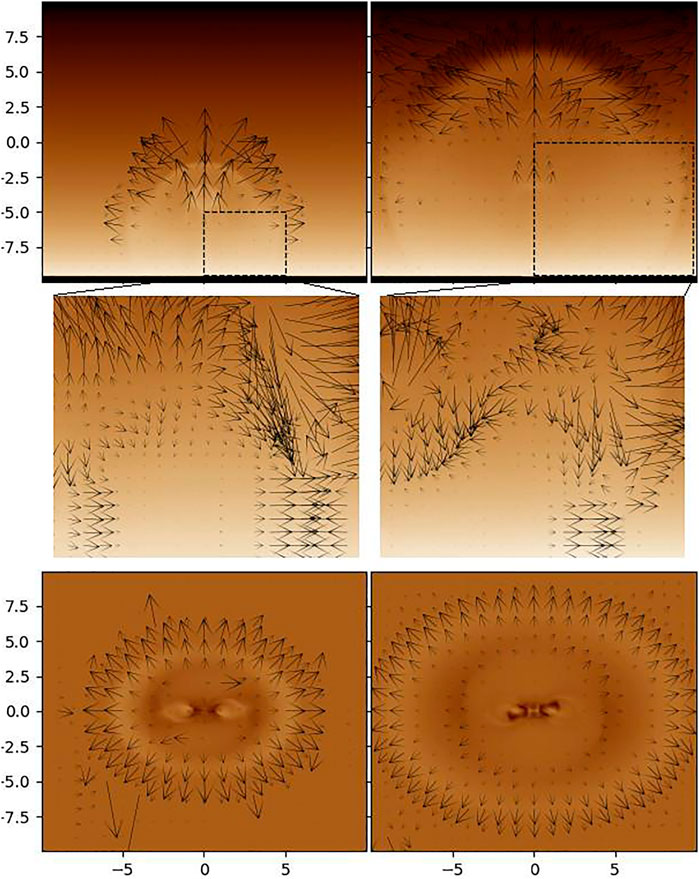
FIGURE 6. Synthetic images of AIA 193Å in the POS in a log-scale with view angles $\mathcal{L}=90°$ and $\mathcal{B}=90°$ (top row) and $\mathcal{L}=0°$ and $\mathcal{B}=0°$ (bottom row) at t = 2 + Δt and 4 + Δt. Here, Δt = 0.0023. The middle low is an enlarged version of two regions marked by two black boxes on the top low. The black arrows illustrate velocity distributions on the POS, which are deduced by the Fourier local correlation tracking software (FLCT) based on the synthetic images.

4 Conclusion

In this work, we have performed a 3D MHD simulation for the EUV disturbance during the eruptions, emphasizing the complex velocity distribution in the lower atmosphere around the eruptive source region. The TD99 model (Titov and Démoulin, 1999) has been used as an initial un-equilibrium magnetic structure, in which a magnetic fluxrope (MFR) models prominence or filament in the corona. An isothermal gravitationally stratified atmosphere has been used to model the background corona. During the MFR eruption, the current sheet (CS) under the MFR grows continuously. The magnetic reconnection inside the CS generates new magnetic field lines to attach to the expanding CME bubble. In front of the CME bubble, the fast shock (FS) and the following helical current boundary (HCB) appear. The HCB comes from the interaction between the CME bubble and the background field. To directly compare with realistic EUV observations, we created synthetic SDO/AIA images for different wavelengths. In synthetic images, the FS moves outward as a 3D dome, followed by the HCS and the MFR, which form the typical three-components CME and may also correspond to the non-wave components of EUV disturbances.

At flanks of the CME bubble, the velocity distribution of the lower atmosphere develops complex structures. Two streams of plasma exist in the lower atmosphere of the eruptive source region, divided by a 3D velocity separatrix (VS). Outside the VS, plasma moves outward to the expanding FS front. Inside the VS, the plasma moves toward the center of the source region. The interaction of two streams of plasma flows has invoked two types of vortexes and the slow shocks (SS) near the VS. The plasma around the first kind of vortex converges to the vortex center. It forms a vortex channel, which lifts plasma nearby the bottom of the simulation box and provides reconnection inflow for the CS and continual plasma for the outermost boundary of the CME bubble. For the second type of vortex, the plasma spreads out from the vortex center, located at higher position than the first kind center, and no associated vortex channel has been observed. In addition, we use the local correlation tracking method to deduce plasma velocity field based on the successive synthetic images. Regrettably, the deduced velocity distributions based on the synthetic images are significantly different from the velocity distribution on the cuts, such as x = 0 and z = z_p shown in Figure 2. For the cases of EUV disturbances observed on the solar disk or the limb, the distribution of deduced velocity shows that almost all plasma moves outward and almost no plasma moves inward, so there is no VS and evidence of the SS. The synthetic image involves the integration of EUV emission along the line-of-sight, so that the deduced velocity can not represent the complex 3D velocity field of plasma during the eruptive events. Thus, it is not easy to find the evidence for the VS, the SS, and the vortex, except we have an in-situ measure datum of eruptive events.

Data Availability Statement

The raw data supporting the conclusion of this article will be made available by the authors, without undue reservation.

Author Contributions

ZM, the corresponding author, performed the numerical simulation setup, numerical algorithm debugging, and data analysis work. QC used the local correlation algorithm to deduce plasma velocity based on synthetic SDO/AIA images. JY contributed to data analysis and physical ideas related to the vortex. BZ and YL gave valuable suggestions on preparing this manuscript. All authors read and approved the submitted version of the manuscript.

Funding

This work was supported by the Strategic Priority Research Program of CAS with grants XDA17040507, the Group for Innovation of Yunnan Province grant 2018HC023, the Yunnan Ten-Thousand Talents Plan-Yunling Scholar Project, the National Science Foundation of China (NSFC) under the grant Nos. 11303088, U2031141 and 12073073 and the Applied Basic Research of Yunnan Province 2019FB005 and 202101AT070018. QC was supported by the Natural Science Foundation of Henan Province 212300410210.

Conflict of Interest

The authors declare that the research was conducted in the absence of any commercial or financial relationships that could be construed as a potential conflict of interest.

Publisher’s Note

All claims expressed in this article are solely those of the authors and do not necessarily represent those of their affiliated organizations, or those of the publisher, the editors and the reviewers. Any product that may be evaluated in this article, or claim that may be made by its manufacturer, is not guaranteed or endorsed by the publisher.

Acknowledgments

We thank the anonymous referee for the valuable comments and suggestions that improved this work and the cluster in the Computational Solar Physics lab of Yunnan Observatories, where we have carried out this simulation.

References

Alexiades, V., Amiez, G., and Gremaud, P.-A. (1996). Super-Time-Stepping Acceleration of Explicit Schemes for Parabolic Problems. Commun. Numer. Meth. Engng. 12, 31–42. doi:10.1002/(sici)1099-0887(199601)12:1<31:aid-cnm950>3.0.co;2-5

CrossRef Full Text | Google Scholar

Asai, A., Ishii, T. T., Isobe, H., Kitai, R., Ichimoto, K., UeNo, S., et al. (2012). First Simultaneous Observation of an Hα Moreton Wave, EUV Wave, and Filament/Prominence Oscillations. ApJ 745, L18. doi:10.1088/2041-8205/745/2/L18

CrossRef Full Text | Google Scholar

Attrill, G. D. R., Harra, L. K., van Driel-Gesztelyi, L., and Démoulin, P. (2007). Coronal "Wave": Magnetic Footprint of a Coronal Mass Ejection? ApJ 656, L101–L104. doi:10.1086/512854

CrossRef Full Text | Google Scholar

Čada, M., and Torrilhon, M. (2009). Compact Third-Order Limiter Functions for Finite Volume Methods. J. Comput. Phys. 228, 4118–4145. doi:10.1016/j.jcp.2009.02.020

CrossRef Full Text | Google Scholar

Chen, P. F., and Wu, Y. (2011). First Evidence of Coexisting Eit Wave and Coronal Moreton Wave from Sdo/Aia Observations. ApJ 732, L20. doi:10.1088/2041-8205/732/2/L20

CrossRef Full Text | Google Scholar

Chen, P. F., Wu, S. T., Shibata, K., and Fang, C. (2002). Evidence of EIT and Moreton Waves in Numerical Simulations. ApJ 572, L99–L102. doi:10.1086/341486

CrossRef Full Text | Google Scholar

Chen, P. F., Ding, M. D., and Fang, C. (2005). Synthesis of CME-Associated Moreton and EIT Wave Features from MHD Simulations. Space Sci. Rev. 121, 201–211. doi:10.1007/s11214-006-3911-0

CrossRef Full Text | Google Scholar

Cheng, X., Zhang, J., Olmedo, O., Vourlidas, A., Ding, M. D., and Liu, Y. (2012). Investigation of the Formation and Separation of an Extreme-Ultraviolet Wave from the Expansion of a Coronal Mass Ejection. ApJ 745, L5. doi:10.1088/2041-8205/745/1/L5

CrossRef Full Text | Google Scholar

Cohen, O., Attrill, G. D. R., Manchester, W. B., Wills-Davey, M. J., and Wills-Davey, M. J. (2009). Numerical Simulation of an Euv Coronal Wave Based on the 2009 February 13 Cme Event Observed Bystereo. ApJ 705, 587–602. doi:10.1088/0004-637x/705/1/587

CrossRef Full Text | Google Scholar

Cunha-Silva, R. D., Selhorst, C. L., Fernandes, F. C. R., and Oliveira e Silva, A. J. (2018). Well-Defined EUV Wave Associated with a CME-Driven Shock. A&A 612, A100. doi:10.1051/0004-6361/201630358

CrossRef Full Text | Google Scholar

Delannée, C., Török, T., Aulanier, G., and Hochedez, J.-F. (2008). A New Model for Propagating Parts of EIT Waves: A Current Shell in a CME. Sol. Phys. 247, 123–150. doi:10.1007/s11207-007-9085-4

CrossRef Full Text | Google Scholar

Downs, C., Roussev, I. I., van der Holst, B., Lugaz, N., and Sokolov, I. V. (2012). Understandingsdo/aia Observations of the 2010 June 13 Euv Wave Event: Direct Insight from a Global Thermodynamic Mhd Simulation. ApJ 750, 134. doi:10.1088/0004-637X/750/2/134

CrossRef Full Text | Google Scholar

Downs, C., Warmuth, A., Long, D. M., Bloomfield, D. S., Kwon, R.-Y., Veronig, A. M., et al. (2021). Validation of Global EUV Wave MHD Simulations and Observational Techniques. ApJ 911, 118. doi:10.3847/1538-4357/abea78

CrossRef Full Text | Google Scholar

Fisher, G. H., and Welsch, B. T. (2008). “FLCT: A Fast, Efficient Method for Performing Local Correlation Tracking,” in Subsurface and Atmospheric Influences on Solar Activity Vol. 383 of Astronomical Society of the Pacific Conference Series. Editors R. Howe, R. W. Komm, K. S. Balasubramaniam, and G. J. D. Petrie (Astronomical Society of the Pacific (ASPC)), 373.

Google Scholar

[Dataset] Fisher, G. H., and Welsch, B. T. (2020). The FLCT Local Correlation Tracking Software. Geneve, Switzerland: Zenodo. doi:10.5281/zenodo.3711569

CrossRef Full Text | Google Scholar

Forbes, T. G. (1990). Numerical Simulation of a Catastrophe Model for Coronal Mass Ejections. J. Geophys. Res. 95, 11919–11931. doi:10.1029/JA095iA08p11919

CrossRef Full Text | Google Scholar

Fulara, A., Chandra, R., Chen, P. F., Zhelyazkov, I., Srivastava, A. K., and Uddin, W. (2019). Kinematics and Energetics of the EUV Waves on 11 April 2013. Sol. Phys. 294, 56. doi:10.1007/s11207-019-1445-3

CrossRef Full Text | Google Scholar

Harten, A. (1983). High Resolution Schemes for Hyperbolic Conservation Laws. J. Comput. Phys. 49, 357–393. doi:10.1016/0021-9991(83)90136-5

CrossRef Full Text | Google Scholar

Jin, M., Manchester, W. B., Holst, B. V. D., Sokolov, I., Tóth, G., Vourlidas, A., et al. (2017). Chromosphere to 1 AU Simulation of the 2011 March 7th Event: A Comprehensive Study of Coronal Mass Ejection Propagation. ApJ 834, 172. doi:10.3847/1538-4357/834/2/172

CrossRef Full Text | Google Scholar

Keppens, R., Meliani, Z., van Marle, A. J., Delmont, P., Vlasis, A., and van der Holst, B. (2012). Parallel, Grid-Adaptive Approaches for Relativistic Hydro and Magnetohydrodynamics. J. Comput. Phys. 231, 718–744. doi:10.1016/j.jcp.2011.01.020

CrossRef Full Text | Google Scholar

Keppens, R., Teunissen, J., Xia, C., and Porth, O. (2020). MPI-AMRVAC: a Parallel, Grid-Adaptive PDE Toolkit. arXiv e-prints , arXiv:2004.03275.

Google Scholar

Kienreich, I. W., Muhr, N., Veronig, A. M., Berghmans, D., De Groof, A., Temmer, M., et al. (2013). Solar TErrestrial Relations Observatory-A (STEREO-A) and PRoject for On-Board Autonomy 2 (PROBA2) Quadrature Observations of Reflections of Three EUV Waves from a Coronal Hole. Sol. Phys. 286, 201–219. doi:10.1007/s11207-012-0023-8

CrossRef Full Text | Google Scholar

Lemen, J. R., Title, A. M., Akin, D. J., Boerner, P. F., Chou, C., Drake, J. F., et al. (2012). The Atmospheric Imaging Assembly (AIA) on the Solar Dynamics Observatory (SDO). SoPh 275, 17–40. doi:10.1007/s11207-011-9776-8

CrossRef Full Text | Google Scholar

Liu, W., and Ofman, L. (2014). Advances in Observing Various Coronal EUV Waves in the SDO Era and Their Seismological Applications (Invited Review). Sol. Phys. 289, 3233–3277. doi:10.1007/s11207-014-0528-4

CrossRef Full Text | Google Scholar

Liu, W., Nitta, N. V., Schrijver, C. J., Title, A. M., and Tarbell, T. D. (2010). First SDO AIA Observations of a Global Coronal EUV “Wave”: Multiple Components and “Ripples”. ApJ 723, L53–L59. doi:10.1088/2041-8205/723/1/L53

CrossRef Full Text | Google Scholar

Liu, W., Title, A. M., Zhao, J., Ofman, L., Schrijver, C. J., Aschwanden, M. J., et al. (2011). Direct Imaging of Quasi-Periodic Fast Propagating Waves of ˜2000 Km S⁻¹ in the Low Solar Corona by the Solar Dynamics Observatory Atmospheric Imaging Assembly. ApJ 736, L13. doi:10.1088/2041-8205/736/1/L13

CrossRef Full Text | Google Scholar

Liu, W., Ofman, L., Nitta, N. V., Aschwanden, M. J., Schrijver, C. J., Title, A. M., et al. (2012). Quasi-periodic Fast-Mode Wave Trains within a Global EUV Wave and Sequential Transverse Oscillations Detected by SDO/AIA. ApJ 753, 52. doi:10.1088/0004-637X/753/1/52

CrossRef Full Text | Google Scholar

Liu, R., Liu, C., Xu, Y., Liu, W., Kliem, B., and Wang, H. (2013). Observation of a Moreton Wave and Wave-Filament Interactions Associated with the Renowned X9 Flare on 1990 May 24. ApJ 773, 166. doi:10.1088/0004-637X/773/2/166

CrossRef Full Text | Google Scholar

Long, D. M., Murphy, P., Graham, G., Carley, E. P., and Pérez-Suárez, D. (2017). A Statistical Analysis of the Solar Phenomena Associated with Global EUV Waves. Sol. Phys. 292, 185. doi:10.1007/s11207-017-1206-0

CrossRef Full Text | Google Scholar

Lugaz, N., Manchester, W. B., Roussev, I. I., Toth, G., and Gombosi, T. I. (2007). Numerical Investigation of the Homologous Coronal Mass Ejection Events from Active Region 9236. ApJ 659, 788–800. doi:10.1086/512005

CrossRef Full Text | Google Scholar

Lugaz, N., Downs, C., Shibata, K., Roussev, I. I., Asai, A., and Gombosi, T. I. (2011). Numerical Investigation of a Coronal Mass Ejection from an Anemone Active Region: Reconnection and Deflection of the 2005 August 22 Eruption. ApJ 738, 127. doi:10.1088/0004-637X/738/2/127

CrossRef Full Text | Google Scholar

Manchester, I., Ward, B., Vourlidas, A., Tóth, G., Lugaz, N., Roussev, I. I., et al. (2008). Three-Dimensional MHD Simulation of the 2003 October 28 Coronal Mass Ejection: Comparison with LASCO Coronagraph Observations. ApJ 684, 1448–1460. doi:10.1086/590231

CrossRef Full Text | Google Scholar

Mei, Z., Udo, Z., and Lin, J. (2012). Numerical Experiments of Disturbance to the Solar Atmosphere Caused by Eruptions. Sci. China Phys. Mech. Astron. 55, 1316–1329. doi:10.1007/s11433-012-4752-3

CrossRef Full Text | Google Scholar

Mei, Z. X., Keppens, R., Roussev, I. I., and Lin, J. (2017). Magnetic Reconnection during Eruptive Magnetic Flux Ropes. A&A 604, L7. doi:10.1051/0004-6361/201731146

CrossRef Full Text | Google Scholar

Mei, Z. X., Keppens, R., Cai, Q. W., Ye, J., Li, Y., Xie, X. Y., et al. (2020a). The Triple-Layered Leading Edge of Solar Coronal Mass Ejections. ApJ 898, L21. doi:10.3847/2041-8213/aba2ce

CrossRef Full Text | Google Scholar

Mei, Z. X., Keppens, R., Cai, Q. W., Ye, J., Xie, X. Y., and Li, Y. (2020b). 3D Numerical Experiment for EUV Waves Caused by Flux Rope Eruption. MNRAS 493, 4816–4829. doi:10.1093/mnras/staa555

CrossRef Full Text | Google Scholar

Meyer, C. D., Balsara, D. S., and Aslam, T. D. (2012). A Second-Order Accurate Super TimeStepping Formulation for Anisotropic thermal Conduction. MNRAS 422, 2102–2115. doi:10.1111/j.1365-2966.2012.20744.x

CrossRef Full Text | Google Scholar

Muhr, N., Veronig, A. M., Kienreich, I. W., Temmer, M., and Vršnak, B. (2011). Analysis of Characteristic Parameters of Large-Scale Coronal Waves Observed by Thesolar-Terrestrial Relations Observatory/Extreme Ultraviolet Imager. ApJ 739, 89. doi:10.1088/0004-637X/739/2/89

CrossRef Full Text | Google Scholar

Muhr, N., Veronig, A. M., Kienreich, I. W., Vršnak, B., Temmer, M., and Bein, B. M. (2014). Statistical Analysis of Large-Scale EUV Waves Observed by STEREO/EUVI. Sol. Phys. 289, 4563–4588. doi:10.1007/s11207-014-0594-7

CrossRef Full Text | Google Scholar

Nisticò, G., Pascoe, D. J., and Nakariakov, V. M. (2014). Observation of a High-Quality Quasi-Periodic Rapidly Propagating Wave Train Using SDO/AIA. A&A 569, A12. doi:10.1051/0004-6361/201423763

CrossRef Full Text | Google Scholar

Pagano, P., Mackay, D. H., and Poedts, S. (2014). Simulating AIA Observations of a Flux Rope Ejection. A&A 568, A120. doi:10.1051/0004-6361/201424019

CrossRef Full Text | Google Scholar

Porth, O., Xia, C., Hendrix, T., Moschou, S. P., and Keppens, R. (2014). MPI-AMRVAC for Solar and Astrophysics. Astrophysical J. Suppl. Ser. 214, 4. doi:10.1088/0067-0049/214/1/4

CrossRef Full Text | Google Scholar

Roussev, I. I., Galsgaard, K., Downs, C., Lugaz, N., Sokolov, I. V., Moise, E., et al. (2012). Explaining Fast Ejections of Plasma and Exotic X-ray Emission from the Solar corona. Nat. Phys. 8, 845–849. doi:10.1038/nphys2427

CrossRef Full Text | Google Scholar

Selwa, M., Poedts, S., and DeVore, C. R. (2012). Dome-Shaped EUV Waves from Rotating Active Regions. ApJ 747, L21. doi:10.1088/2041-8205/747/2/L21

CrossRef Full Text | Google Scholar

Shen, Y., and Liu, Y. (2012). Evidence for the Wave Nature of an Extreme Ultraviolet Wave Observed by the Atmospheric Imaging Assembly on Board Thesolar Dynamics Observatory. ApJ 754, 7. doi:10.1088/0004-637X/754/1/7

CrossRef Full Text | Google Scholar

Shen, Y., Liu, Y., Su, J., Li, H., Zhao, R., Tian, Z., et al. (2013). Diffraction, Refraction, and Reflection of an Extreme-Ultraviolet Wave Observed during its Interactions with Remote Active Regions. ApJL 773, L33. doi:10.1088/2041-8205/773/2/L33

CrossRef Full Text | Google Scholar

Shen, Y., Chen, P. F., Liu, Y. D., Shibata, K., Tang, Z., and Liu, Y. (2019). First Unambiguous Imaging of Large-Scale Quasi-Periodic Extreme-Ultraviolet Wave or Shock. ApJ 873, 22. doi:10.3847/1538-4357/ab01dd

CrossRef Full Text | Google Scholar

Thompson, B. J., and Myers, D. C. (2009). A Catalog of Coronal “EIT Wave” Transients. Astrophysical J. Suppl. Ser. 183, 225–243. doi:10.1088/0067-0049/183/2/225

CrossRef Full Text | Google Scholar

Titov, V. S., and Démoulin, P. (1999). Basic Topology of Twisted Magnetic Configurations in Solar Flares. A&A 351, 707–720.

Google Scholar

Uchida, Y. (1970). Diagnosis of Coronal Magnetic Structure by Flare-Associated Hydromagnetic Disturbances. PASJ 22, 341.

Google Scholar

Van Doorsselaere, T., Antolin, P., Yuan, D., Reznikova, V., and Magyar, N. (2016). Forward Modeling of EUV and Gyrosynchrotron Emission from Coronal Plasmas with FoMo. Front. Astron. Space Sci. 3, 4. doi:10.3389/fspas.2016.00004

CrossRef Full Text | Google Scholar

Vršnak, B., and Cliver, E. W. (2008). Origin of Coronal Shock Waves. Sol. Phys. 253, 215–235. doi:10.1007/s11207-008-9241-5

CrossRef Full Text | Google Scholar

Wang, H., Shen, C., and Lin, J. (2009). Numerical Experiments of Wave-Like Phenomena Caused by the Disruption of an Unstable Magnetic Configuration. ApJ 700, 1716–1731. doi:10.1088/0004-637X/700/2/1716

CrossRef Full Text | Google Scholar

Wang, H., Liu, S., Gong, J., Wu, N., and Lin, J. (2015). Contribution of Velocity Vortices and Fast Shock Reflection and Refraction to the Formation of EUV Waves in Solar Eruptions. ApJ 805, 114. doi:10.1088/0004-637X/805/2/114

CrossRef Full Text | Google Scholar

Wang, C., Chen, F., and Ding, M. (2021). Exploring the Nature of EUV Waves in a Radiative Magnetohydrodynamic Simulation. ApJL 911, L8. doi:10.3847/2041-8213/abefe6

CrossRef Full Text | Google Scholar

Warmuth, A. (2015). Large-Scale Globally Propagating Coronal Waves. Living Rev. Sol. Phys. 12, 3. doi:10.1007/lrsp-2015-3

PubMed Abstract | CrossRef Full Text | Google Scholar

Wills‐Davey, M. J., DeForest, C. E., and Stenflo, J. O. (2007). Are "EIT Waves" Fast‐Mode MHD Waves? ApJ 664, 556–562. doi:10.1086/519013

CrossRef Full Text | Google Scholar

Xia, C., and Keppens, R. (2016). Formation and Plasma Circulation of Solar Prominences. ApJ 823, 22. doi:10.3847/0004-637X/823/1/22

CrossRef Full Text | Google Scholar

Xia, C., Teunissen, J., Mellah, I. E., Chané, E., and Keppens, R. (2018). MPI-AMRVAC 2.0 for Solar and Astrophysical Applications. ApJS 234, 30. doi:10.3847/1538-4365/aaa6c8

CrossRef Full Text | Google Scholar

Xie, X., Mei, Z., Huang, M., Lv, Q., Roussev, I. I., and Lin, J. (2019). Numerical Experiments of Various Types of Disturbances in the Low and Middle corona Caused by Solar Eruptions. MNRAS 490, 2918–2935. doi:10.1093/mnras/stz2576

CrossRef Full Text | Google Scholar

Ye, J., Cai, Q., Shen, C., Raymond, J. C., Lin, J., Roussev, I. I., et al. (2020). The Role of Turbulence for Heating Plasmas in Eruptive Solar Flares. ApJ 897, 64. doi:10.3847/1538-4357/ab93b5

CrossRef Full Text | Google Scholar

Zhao, X., Xia, C., Doorsselaere, T. V., Keppens, R., and Gan, W. (2019). Forward Modeling of SDO/AIA and X-Ray Emission from a Simulated Flux Rope Ejection. ApJ 872, 190. doi:10.3847/1538-4357/ab0284

CrossRef Full Text | Google Scholar

Zheng, R., Chen, Y., Feng, S., Wang, B., and Song, H. (2018). An Extreme-Ultraviolet Wave Generating Upward Secondary Waves in a Streamer-Like Solar Structure. ApJ 858, L1. doi:10.3847/2041-8213/aabe87

CrossRef Full Text | Google Scholar

Zhou, Y.-H., Ruan, W.-Z., Xia, C., and Keppens, R. (2021). Transition Region Adaptive Conduction (TRAC) in Multidimensional Magnetohydrodynamic Simulations. A&A 648, A29. doi:10.1051/0004-6361/202040254

CrossRef Full Text | Google Scholar