 K-J. Hwang1*
 K. Dokgo1
 E. Choi1
 J. L. Burch1
 D. G. Sibeck2B. L. Giles2
 C. Norgren3
 T. K. M. Nakamura4,5
 D. B. Graham6
 Y. Khotyaintsev6Q. Q. Shi7D. J. Gershman2C. J. Pollock8R. E. Ergun9R. B. Torbert10C. T. Russell11R. J. Strangeway11
- 1Southwest Research Institute, San Antonio, TX, United States
- 2NASA Goddard Space Flight Center, Greenbelt, MD, United States
- 3Department of Physics and Technology, University of Bergen, Bergen, Norway
- 4Institute of Physics, University of Graz, Graz, Austria
- 5Austrian Academy of Sciences ÖAW, Space Research Institute, Graz, Austria
- 6Swedish Institute of Space Physics, Uppsala, Sweden
- 7School of Earth and Space Sciences, Peking University, Peking, China
- 8Denali Scientific, LLC, Fairbanks, AK, United States
- 9Laboratory for Atmospheric and Space Physics, University of Colorado at Boulder, Boulder, CO, United States
- 10Space Science Center, University of New Hampshire, Durham, NH, United States
- 11Institute of Geophysics and Planetary Physics, University of California, Los Angeles, CA, United States
On May 5, 2017 MMS observed a bifurcated current sheet at the boundary of Kelvin-Helmholtz vortices (KHVs) developed on the dawnside tailward magnetopause. We use the event to enhance our understanding of the formation and structure of asymmetric current sheets in the presence of density asymmetry, flow shear, and guide field, which have been rarely studied. The entire current layer comprises three separate current sheets, each corresponding to magnetosphere-side sunward separatrix region, central near-X-line region, and magnetosheath-side tailward separatrix region. Two off-center structures are identified as slow-mode discontinuities. All three current sheets have a thickness of ∼0.2 ion inertial length, demonstrating the sub-ion-scale current layer, where electrons mainly carry the current. We find that both the diamagnetic and electron anisotropy currents substantially support the bifurcated currents in the presence of density asymmetry and weak velocity shear. The combined effects of strong guide field, low density asymmetry, and weak flow shear appear to lead to asymmetries in the streamlines and the current-layer structure of the quadrupolar reconnection geometry. We also investigate intense electrostatics waves observed on the magnetosheath side of the KHV boundary. These waves may pre-heat a magnetosheath population that is to participate into the reconnection process, leading to two-step energization of the magnetosheath plasma entering into the magnetosphere via KHV-driven reconnection.
Introduction
About sixty years ago Dungey (1961) and Axford and Hines (1961) proposed two different models of the solar wind-magnetosphere interaction. The former was based on the concept of magnetic reconnection under large magnetic field shear. The latter was on quasi-viscous interaction in the boundary layer powered by large flow velocity shear. Since then two most important physical processes that lead and regulate the solar wind-Earth’s magnetosphere coupling are thought to be magnetic reconnection and the Kelvin-Helmholtz instability (KHI).
Both processes exhibit multi-scale features and either compete or enhance each other. Magnetic reconnection is initiated on the electron-scale size, i.e., in the electron diffusion region (EDR) and then entails dynamics in the ion diffusion region (IDR), and ultimately propagates its effect to the macroscopic region where magnetohydro-dynamics (MHD) governs. On the other hand, Kelvin-Helmholtz waves (KHWs) occurring on the Earth’s magnetopause are often generated on the macroscopic scales, i.e., ∼1 RE (Earth radii) (Hasegawa et al., 2004) and then involve kinetic processes occurring on the ion and electron scales as the waves nonlinearly grow into Kelvin-Helmholtz vortices (KHVs). The vortex motion facilitates the formation of thin current sheets between stretched magnetosheath and magnetospheric field lines at the edge of KHVs where magnetic reconnection can occur (Nykyri and Otto, 2001, 2004). Observations (Fairfield et al., 2000; Nykyri et al., 2006; Eriksson et al., 2009, 2016; Hasegawa et al., 2009; Li et al., 2016; Hwang et al., 2020; Kieokaew et al., 2020) have reported ongoing reconnection in such a thin current sheet developed along the boundary of KHVs or a magnetic island as predicted by simulations (Nakamura et al., 2013, 2017). Magnetic reconnection at the edge of KHVs and/or a wave packet inside KHVs (Moore et al., 2016) result in cross-scale energy transport.
Cassak and Otto (2011) showed that a flow shear across the symmetric reconnection current sheet decreases the efficiency of the reconnected field line to drive the outflow, similarly to the suppression of reconnection by the diamagnetic effect (Swisdak et al., 2003, 2010). They used the full particle simulation to derive that the reconnection-cutoff velocity shear is the upstream Alfvén speed. Doss et al. (2015) studied the effect of the flow shear in asymmetric reconnection, analytically and numerically predicting that the asymmetric effect allows reconnection to continue even for super-Alfvénic upstream velocity shear. Tanaka et al. (2010) further considered the effect of a guide field as well as a flow shear in asymmetric reconnection, reporting that both an initial upstream flow and the Lorentz force acting inflowing plasmas in the presence of a guide field produce a slanted inflow to the current sheet. Resulting asymmetries in the quadrupolar reconnection current layer is qualitatively similar to the MHD simulation by La Belle-Hamer et al. (1995).
The 2-D MHD simulation for the current sheet across which substantial velocity shear and density jump exist (La Belle-Hamer et al., 1995) indicates that depending on either the competition (occurring on the tailward exhaust region) or the enhancement (sunward exhaust) of the two velocity-shear and densty-asymmetry effects, the structure of the current sheet is often different from the simple 1-D Harris model, showing double off-center peaks in current, i.e., current bifurcation. The bifurcated current sheet has been understood as the Petschek-type reconnection layer, where the reconnection outflow jets ejected from the X-line are bounded by two rotational discontinuities or slow mode shock structures, which split a single reconnecting current sheet.
On the other hand, bifurcated current sheets observed in Earth’s magnetotail are often not necessarily associated with fast flows (Asano et al., 2003). Numerous studies have been put forth to understand the formation of such bifurcated magnetotail current-sheets, attributing its cause to flapping of the current sheet (Sergeev et al., 2003), magnetic turbulence (Greco et al., 2002), Kelvin-Helmholtz instability (Nakagawa and Nishida, 1989; Yoon, Drake and Lui, 1996), Ion-ion kink instability (Karimabadi et al., 2003), temperature anisotropy (Sitnov et al., 2004; Zelenyi et al., 2004) or relaxation processes of a disequilibrated current sheet, in particular, during current sheet thinning or quasi-steady compression (Schindler and Hesse, 2008; Jiang and Lu, 2021; Yoon et al., 2021).
The formation and structure of asymmetric current sheets in the presence of flow shear, density asymmetry, and guide field have been much less studied. In particular, despite the prediction by La Belle-Hamer et al. (1995), evidence of bifurcated current sheets in KHW/KHV-induced reconnecting layers is rarely reported to this day. The only observation by Cluster (Hasegawa et al., 2009) showed that each of the two current sheets constituting the bifurcated layer had a thickness less than the ion inertial length and that the current was likely supported by electrons.
To enhance our understanding of the properties of the magnetic reconnection layer under the combined sheared plasma flow, guide field, and density asymmetry, i.e., typically occurring on the flank-side magnetopause, we use the data from MMS on May 5, 2017. In this paper, we present the observation of a bifurcated current sheet identified on the boundary of KHVs. The following paragraph briefly describes the MMS instruments and data analysis techniques used for the present study (Methods Section). We then investigate plasma and field properties associated with the bifurcated and central current sheets and show that the electrons drifting under both the diamagnetic effect and the magnetic curvature with large temperature anisotropy significantly contribute to the current (The Structure of Current Sheets Section). We also investigate intense electrostatics waves that are predominantly observed on the magnetosheath side of the central current layer (Wave Observation and Analysis Section). Discussion of the formation and structure of the observed current sheet in the presence of flow shear, density asymmetry, and guide field, and the implied cause and effect of the enhanced waves follow in Discussion Section.
Methods
The four MMS spacecraft (Burch et al., 2016a) fly in low-inclination and highly elliptical orbits. We used the magnetic field data with a time resolution of 10-ms in burst mode, the electric field data with a 0.122-ms time resolution in burst mode, and ion and electron data in burst mode with a 150-ms and 30-ms time resolution, respectively, a 11.25° angular resolution, and an energy range of ∼10 eV–26 keV.
We determined boundary normal coordinates (LMN) by performing minimum directional derivative (MDD) analysis (Shi et al., 2005): three eigenvectors corresponding to the medium, minimum, and maximum eigenvalues (
The Structure of Current Sheets
From 1920 to 2320 UT on May 5, 2017, MMS observed quasi-periodic perturbations of the dawnside tailward magnetopause, as reported by Hwang et al. (2020). Figure 1A shows (i) the interplanetary magnetic field obtained from ACE OMNI-HRO 1-min data and (ii) the magnetic field at dawnside tailward magnetopause encountered by MMS4 (x, y, and z components in blue, green, and red with the magnetic strength in black) during 1930–2100 UT in Geocentric Solar Magnetospheric (GSM) coordinates. The ACE HRO data provide the time-shifted IMF (interplanetary magnetic field) at a model bow shock nose location (Russell et al., 1983).
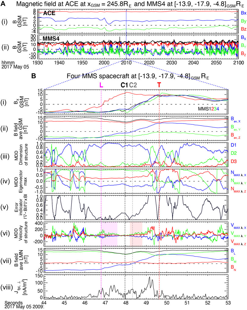
FIGURE 1. (A) (i) the interplanetary magnetic field obtained from ACE OMNI-HRO 1-min data and (ii) the magnetic field at dawnside tailward magnetopause encountered by MMS4 (x, y, and z components in blue, green, and red with the magnetic strength in black) during 1930–2100 UT on May 5 2017 in Geocentric Solar Magnetospheric (GSM) coordinates. (B) The four MMS observations on May 5 2017 during 2009:44–53 UT: (i) the x component of the magnetic field (B) in GSM measured at MMS1 (black), 2 (red), 3 (green), and 4 (red); (ii) the tetrahedral-averaged B in GSM; MDD (Shi et al., 2005; 2006)-derived (iii) dimensionality of the structure, (iv) the eigenvector corresponding to the maximum eigenvalue of the matrix,
The event occurred within a period of mainly northward and slightly sunward/dawnward IMF (Figures 1Ai). MMS4 observed quasi-periodic fluctuations with a period of ∼2.5–6 min (Figures 1Aii). Hwang et al. (2020) showed via boundary-normal analyses that the fluctuations were likely to be attributed to nonlinear KHWs. During this internal, we identified a thin current sheet formed at the boundary of the KHV at ∼2009:49 UT (the vertical blue line in Figure 1A) when MMS traversed the boundary from the magnetospheric side to the magnetosheath side.
Figures 1Bi shows the x component of the magnetic field (B) in GSM coordinates. The negative-to-positive reversal of Bx observed by MMS1, 2, 3, and 4 (black, red, green, and blue) indicates a current sheet. The Bx profiles are, however, different from a Harris-sheet hyperbolic tangent profile, displaying local dip and peak and plateau (MMS2) or gentle slope (MMS134) between them, indicative of a bifurcated current sheet.
Figures 1Bii shows a 4-spacecraft tetrahedral-averaged B, which emphasizes the plateau around the center of the current sheet, marked by “C1” at the top of Figures 1Bi and the vertical dashed black line. MDD and STD analyses (Methods Section) derive the dimensionality and motional velocity of the structure and its boundary-normal direction (Figures 1Biii–vi). The overall current-sheet structure between the leading (“L” on the top of Figures 1Bi and vertical dashed magenta line) and trailing (“T” and vertical dashed red line) edges is mostly 1-D (Figures 1Biii), but significantly 2-D toward the trailing edge.
The current-sheet-normal vector is mainly along yGSM (Figures 1Biv), as expected for the flank-side magnetopause. The three eigenvectors of
Figure 2A shows the tetrahedral configuration of the four MMS spacecraft in LMN around its barycenter at (−13.9, −17.9, −4.8)GSM Earth radii (RE). The notable difference in Bx between MMS2 and MMS134 (Figures 1Bi) most likely came from the n-directional separation, as seen in their LN-plane projections. About 179 km separation along n as well as the average spacecraft separation of ∼156 km/s are comparable to the ion inertial length (di) based on the magnetosheath values (di = ∼185 km).
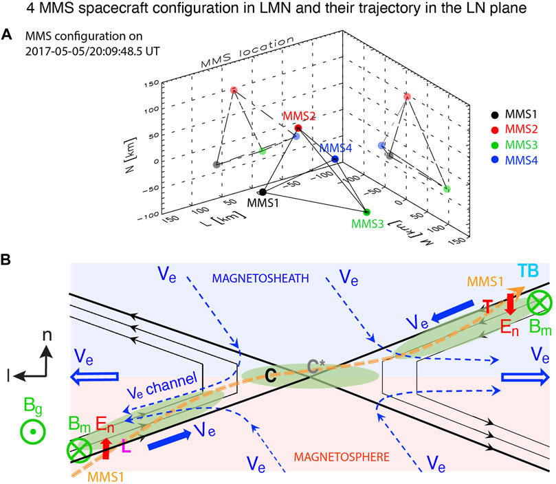
FIGURE 2. (A) The tetrahedral configuration of the four MMS spacecraft around its barycenter at (−13.9, −17.9, −4.8)GSM Earth radii (RE) on 2009:48/5 UT; (B) the illustration of the trajectory of MMS1 (the dashed orange arrow) across the reconnection plane, where “L”, “C”, “C*”, and “T” correspond to those shown at the top of Figure 3.
Figures 1Bvii shows the tetrahedral-averaged B in LMN. The negative-to-positive Bl reversal is denoted by “C2” and the vertical dashed gray line. The tetrahedral-averaged electric current calculated from particle moments perpendicular to B (Figures 1Bviii) shows three overall peaks between “L” and “T”. They comprise two larger peaks before and after “C2” and a smaller peak at ∼”C2”. Using the STD-driven current-sheet normal velocity (Figures 1Bvi), we estimate the thickness of each current sheet. The averaged normal velocity during 2009:46.8–47.5 UT and during 2009:48.2–48.8 UT (with an error indicator less than 0.5) (magenta and red shades in Figures 1Bvi) is (−8.6, −1.0, −64.5) km/s and (−11.6, 8.2, −67.8) km/s in LMN, respectively. This is relatively consistent with the result derived from a four-spacecraft timing analysis based on the time difference in the Bx reversal among the four spacecraft (Figures 1Bi): (−21.5, −1.68, −68.0) km/s. We assume the overall current-sheet-normal velocity to be 67 km/s along -n. Then, the three current sheets before, at/around, and after “C2” with a duration of ∼0.65, 0.50, and 0.65 s (Figures 1Bviii and Figure 4B) has a thickness of ∼43.6, 33.5, and 43.6 km. Since these values correspond to ∼0.24, 0.18, and 0.24 di (∼9.7, 7.4, and 9.7 electron inertial length, de ∼ 4.5 km in this event) similar to Hasegawa et al. (2009), the current in these sub-ion scale current sheets is expected to be supported by electrons.
Due to the large spacecraft separation compared to the current sheet thickness, investigation of the detailed structure of the current layer should be made using an individual spacecraft. We use the data from MMS1 (Figure 3 with all vector parameters in LMN). Figures 3A,B shows the l (blue), m (green), and n (red) components of the magnetic (B) and electric (E) fields. The leading and trailing edges (“L” and “T”, magenta and red dashed lines) denote dip and hump in Bl, decreases in Bm, and increase (
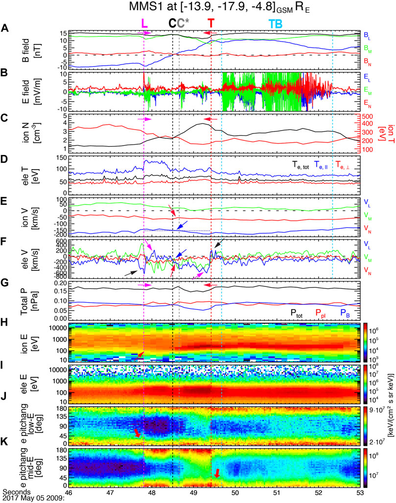
FIGURE 3. MMS1 observation on May 5,2,017 during 2009:46–53 UT: (A,B) the l (blue), m (green), and n (red) components of the magnetic field (B) and the electric field (E) in LMN; (C) the ion density (black) and temperature (red); (D) the electron total (black), parallel (bule), and perpendicular (red) temperature; (E) the ion velocity; (F) the electron velocity; (G) the plasma (red) and magnetic (blue) pressures, and the sum (black) of these pressures; (H) the ion energy spectrogram; (I) the electron energy spectrogram; (J,K) pitch angle distributions of the low- (∼10 eV ≤ energy <200 eV; J), mid- (200 eV ≤ energy <2 keV; K) energy electrons.
Variations of the ion density and ion/electron temperatures (Figures 3C,D) together with ion/electron energy spectrograms (Figures 3H,I) show that MMS1 crossed the current sheet from the more magnetospheric region (prior to “C”) to the more magnetosheath region (after “C”). Intense electric field fluctuations (marked by “TB” and two vertical dashed cyan lines) are seen in the magnetosheath side of the current sheet (to be discussed in Wave Observation and Analysis Section).
The ion velocity between “L” and “T” varies from slower tailward flow (smaller −Vi,l) to faster tailward flow (larger −Vi,l) across “C” (marked by the blue arrow in Figure 3E) around Vi,l = −154 km/s (the blue dotted line). This indicates the sunward exhaust region (before “C”) to the antisunward exhaust region (after “C”) of the current sheet, which was convecting antisunward along with the KHV propagation.
Therefore, MMS most likely crossed the overall current sheet from the sunward magnetospheric quadrant to the antisunward magnetosheath quadrant of the reconnection plane with a large guide field, Bg (Bm) ∼ 1.5 |Bl| (at 2009:46.0 UT; Figure 3A) out of the plane. The trajectory of MMS is denoted by the dashed orange arrow in Figure 2B, where “L”, “C”, “C*”, and “T” correspond to those shown at the top of Figure 3A. The aforementioned Hall magnetic and electric field signatures are illustrated in green and red, respectively, around “L” and “T”.
The electron velocity shows more complicated patterns than the ion velocity. Beyond the same variation of the slower-to-faster tailward outflow jets across “C” (blue arrow in Figure 3F), the slower tailward flow between “L” and “C” includes a short duration of the sunward flow (+Ve,l) during 2009:47.9–48.1 UT (magenta arrow). This indicates the existence of a narrow (∼13.4 km, ∼3 de) electron-current layer embedded in the outflow region (marked by “Ve channel” in Figure 2B). Its counterpart may exist in the tailward exhaust region (between “C” and “T”) with a faster tailward jet before “T” (magenta arrow in Figure 3F). Figure 2B shows possible electron flow streamlines in dashed blue arrows that may explain the observed flow channels.
Around “L” and “T”, Ve,l sharply changes its sign. The enhanced tailward flow before/at ‘L’ and the sunward flow at/after “T” (black arrows in Figure 3F) are associated with electrons streaming toward an X-line in the separatrix region (see solid blue arrows in Figure 2B) (Egedal et al., 2005, 2008; Hwang et al., 2017, 2018). Pitch-angle distributions of the low- (<200 eV) and mid- (200 eV < energy <2 keV) energy electrons support this, showing the enhancement of the parallel flux at/around “L” and “T” (red arrows in Figures 3J,K). These counter-streaming electron flows (±Ve,l) across ∼“L” and ∼“T” sustain the Hall field along the separatrix.
These electron populations carry the electric current (current density, J) around “L” and “T”. Figure 4B shows the l, m, and n components of J calculated from both ion and electron moments (solid blue, green, and red profiles). Overplotted are the ion current (dot-dashed light blue, light green, and orange) and the electron current (dotted blue, dark green, and red). The current (in particular, Jm) is mostly carried by electrons. Both Jl and Jm between “L” and “T” show the three-peak structure with two larger peaks before/after “C” and a smaller peak located at the Bn reversal (“C*”), as demonstrated in J|| (black arrows in Figure 4C). Thus, we speculate that the two larger peaks correspond to one of each pair of a bifurcated current sheet and the central peak is associated with an X-line (Figure 2B).
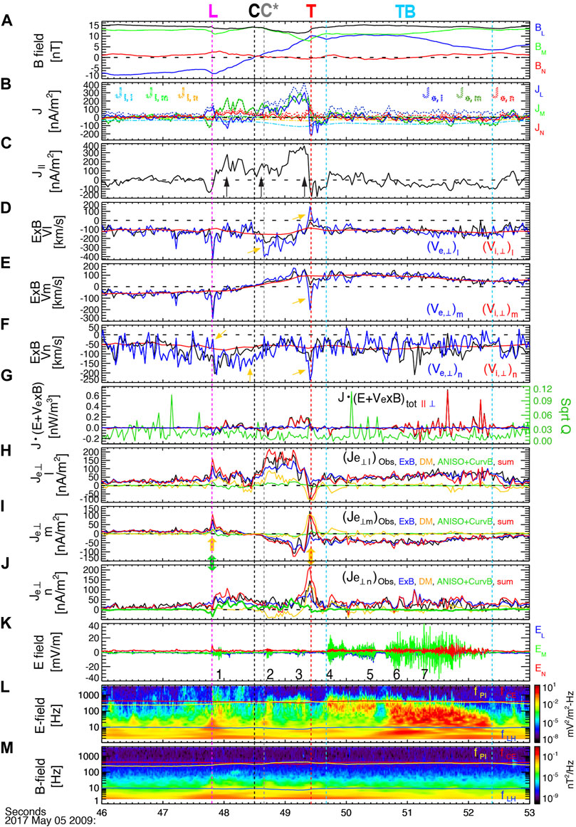
FIGURE 4. MMS1 observation on May 5 2017 during 2009:46–53 UT: (A) the l (blue), m (green), and n (red) components of B; (B) the l, m, and n components of the current density (J) calculated from both ion and electron moments (solid blue, green, and red profiles), the ion current (dot-dashed blue, green, and orange), and the electron current (dotted blue, darkgreen, and orange); (C) the current density parallel to B; (D–F) the l, m, and n components of the
In the sub-ion scale current layers such as this event, ion velocities perpendicular to B can be different from the
To see the level of electron agyrotropy, we use
To understand the electron deviation from
Wave Observation and Analysis
We investigate the intense waves observed intermittently within the current layer (marked by 1, 2, and 3 in Figure 4K and stronger wave activities (throughout 4–7) observed during “TB”. Figures 4L,M show the power spectral density (PSD) of E and B. The waves are mostly electrostatic and enhanced near or below the electron cyclotron frequency (fCE) or the ion plasma frequency (fPI) and above the lower-hybrid frequency (fLH).
Figure 5i shows the waveform of E decomposed into parallel (red) and perpendicular (blue) components with respect to B for timing 1, 4, and 7 (Figure 4K). To estimate the propagation direction (
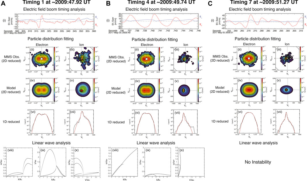
FIGURE 5. Analysis of the waves observed at timing, 1 (A), 4 (B), and 7 (C) marked in Figure 4K: (i) the electric field decomposed into the parallel (red) and perpendicular (blue) components to B; (ii,iii) MMS observations of 2-D reduced electron (ii) and ion (iii) distributions in the
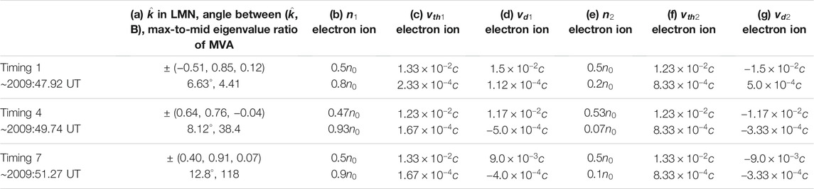
TABLE 1. Parameters of modeled distributions used for linear analysis, where
To understand the generation of theses waves, we perform linear instability analysis using the electron and ion distribution functions at timing 1, 4, and 7. Each particle distribution is modeled by a sum of two Maxwellian distributions, and the best fitting parameters (density, thermal speed, and beam drift speed) are listed in Table 1 (b–g). Figure 5ii–v shows MMS observations of 2-D reduced electron (ii) and ion (iii) distributions and their 2-D reduced model distributions (iv, v) in the
By making use of these modeled-distribution parameters (Table 1 b–g), we perform the linear kinetic instability analysis using BO code (Xie, 2019). Figures 5viii–ix show real and imaginary parts of the growing mode in
At timing 1, a low-frequency mode is generated in the range of
At timing 4, the frequency range of wave generation is much broader than timing 1. Two distinct modes are derived. One locates below
At timing 7, the modeled distribution produces no growing mode most likely due to the flattened electron distribution. This indicates that the bi-directional electron beams are a major free-energy source for the generation of the observed electrostatic waves.
Discussion
In this paper, we report a bifurcated current sheet developed on the boundary of KHVs propagating along the flank-side magnetopause, across which both plasma flow shear and density asymmetry exist under a large guide field, Bg ∼ 1.0 |Bl| (on the magnetosheath side) to 1.5 |Bl| (on the magnetospheric side). Via discussion on The Structure of Current Sheets Section, we speculate the trajectory of MMS that followed the dashed orange arrow in Figure 2B across the reconnection plane.
The overall current density profiles show three peaks (Figures 4K,L; green shades in Figure 2B), each observed in the proximity to the magnetospheric-side, sunward separatrix region (around “L”), the central, near-X-line region (“C-C*”), and the magnetosheath-side, tailward separatrix region (around “T”). The slower-tailward to faster-tailward jets across the central current sheet, i.e., reconnection outflows, demonstrate that the two off-centered signatures are corresponding to two rotational discontinuities or slow mode shocks in the Petschek reconnection geometry. 1) Tangential (Bl) and normal (Bn) components of B are non-zero at/around “L” and “T”. 2) Decrease in |Bl| from upstream (inflow region) to downstream (outflow region) of “L” and “T” (along magenta and red arrows in Figure 3A) indicates that the magnetic field bends toward n. 3) The magnetic field strength or pressure decrease from upstream to downstream (magenta and red arrows in Figures 3A,G). 4) The plasma density and pressure increase (magenta and red arrows in Figures 3C,G) across “L” and “T”. All 1–4) features support that the two discontinuities are identified as slow modes.
For the two periods between “L” and ∼“C” and between ∼“C” and “T”, we performed a Walén test separately for ions and electrons (Scudder et al., 1999; Hwang et al., 2016). The ion flow in the deHoffmann-Teller frame (
Lin and Lee (1994), for asymmetric guide-field reconnection with no velocity shear, predicted the formation of different discontinuities between on the magnetosheath-side separatrix region (a time-dependent intermediate shock and a slow expansion wave, which evolves to a slow shock with time) and the magnetospheric-side separatrix region (a time-dependent intermediate shock and a weak slow shock). Such multiple discontinuities were not observed in this event, where the whole current layer is on a sub-ion scale, i.e., possibly due to the MMS trajectory being too close to the X-line. Further comparison is hindered since MMS did not traverse the entire exhaust region either side of X. The MHD simulation (La Belle-Hamer et al., 1995) for asymmetric no-Bg reconnection with a flow shear also predicted the formation of an intermediate shock on the magnetosheath-side, sunward separatrix region (the upper-left quadrant of Figure 2B), which was, again, not traversed by MMS.
We note a short duration of the sunward electron jet between “L” and “C”. Ve,n and Vi,n are more negative and less negative across “C” (red arrows in Figure 3F). Thus, the plasma streamlines between “L”−“C” and “C”−“T” might not be symmetric (dashed blue arrows in Figure 2B).
La Belle-Hamer et al. (1995) and Tanaka et al. (2010), indeed, predicted such asymmetry in the reconnection geometry under the density gradient and velocity shear. In the tailward exhaust region (i.e., between “C*” and “T”), the outflow (
In the sunward magnetosheath-side exhaust region, the outflow (
It may be notable that although such asymmetric streamlines are indicated by ion flows in the MHD (La Belle-Hamer et al., 1995) and particle-in-cell (Tanaka et al., 2010) simulations, the electron velocity appears to mostly represent the asymmetry in the present event. This implies that the aforementioned combined effects of the shear flow and density asymmetry are valid for the electron streamlines, in particular, in this sub-ion scale current layer.
We also note that the upstream flow difference across the current sheet is quite weak in this event (∼6% of the parallel Alfvén speed on either side of the current sheet) while Bg is strong. Tanaka et al. (2010) showed that the combination of density gradient and guide field led to the similar effect obtained by the combination of density gradient and flow shear. Thus, we conclude that the combined effects of strong guide field, low density asymmetry (
We estimate how these asymmetries would modify the reconnection rate, using the formula derived by Doss et al. (2015):
where
Electrons mainly carried the current for the present event, and ion contribution to the currents is limited up to ∼27% of the total current (Figure 4B), which is expected for the sub-ion scale current sheet. The three current density humps have a thickness of ∼43.6, 33.5, and 43.6 km, i.e., ∼0.24, 0.18, and 0.24 di (∼9.7, 7.4, and 9.7 de), respectively, demonstrating the sub-ion scale current layer.
Numerous theoretical and simulation studies for the magnetotail (i.e., symmetric) environment have been performed to understand the formation of the current sheet bifurcation. Among various mechanisms proposed, one important factor is temperature anisotropy. Sitnov et al. (2004) suggested that the bifurcation is caused by weak ion temperature anisotropy with
In our observation, we note the opposite electron anisotropy,
A statistical study of the bifurcated current sheets using Cluster data (Thompson et al., 2006) indicated that the narrower the current sheets are, the more likely they are bifurcated. This, together with our present study, may suggest that the electrons play a major role in the formation of the bifurcated current sheet in both symmetric and asymmetric environment.
We investigated intense electrostatics waves that were predominantly observed on the magnetosheath side of the central current layer using linear kinetic analysis for selected timings, 1, 4, and 7 (Figure 4K). At timing 1 and 4, the electron distributions contain clear bi-directional beams with growing wave modes produced, while at timing 7 they show a plateau distribution with no growing mode wave. Still, large differences in the wave generation between timing 1 and 4 imply that various types of waves could be generated by the bi-directional beams that are ubiquitous in the KHV-induced reconnection sites (Wilder et al., 2016; Hwang et al., 2020).
Unlike the linear kinetic instability theory, we observed the electrostatic wave at timing 7. The waveforms at timing 7 (Figures 5Ci), however, indicate highly nonlinear waves. They are possibly propagated to the MMS location, after having been generated remotely. We also note that the first wave signature observed near “L” or 1 in Figure 4K corresponds to the location where the low-energy (cold) magnetosheath ion reaches after penetrating into the magnetospheric side, as indicated by the plasma density (black in Figure 3C) and the red arrow in Figure 3H.
Therefore, we speculate that ion may play an important role in generating different types of waves. According to Omura et al. (1996), ions could change types of generated waves depending on the ion temperature and the ion drift by interacting resonantly with waves generated by electrons or scattering electrons. As a result, various types of waves could be generated such as ion acoustic wave, electron solitary wave, electron hole, and Langmuir wave. Nonlinear wave mode and its evolution cannot be studied by linear analysis. Further study using kinetic simulation is required for understanding how ion dynamics affect nonlinear wave mode.
This observation, however, implies that the electrostatic waves observed predominantly in the magnetospheath side of the KHV boundary may pre-heat the cold magnetosheath population that is to participate into the reconnection process moving toward an X-line via/along the inflow/separatrix region. This may explain the higher-energy (200 eV < energy <2 keV) electrons streaming toward X along the magnetosheath-side separatrix region (red arrow in Figure 3K). Large Joule dissipation during the period of the enhanced wave activity (Figure 4G) also supports this two-step energization of the magnetosheath plasma entering into the magnetosphere via KHV-driven reconnection.
Data Availability Statement
The datasets presented in this study can be found in online repositories. The names of the repository/repositories and accession number(s) can be found in the article/Supplementary Material.
Author Contributions
K-JH led the investigation including data analysis and interpretation, and produced the manuscript with Figures. KD, EC, LB, DS, CN, KN, and DBG participated in the data analysis. BG, YK, DJG, CP, RE, RT, CT, and RS provided the data, assisting the validation of the data use and interpretation. QS and DBG provided the analysis tool.
Funding
This study was supported, in part, by NASA’s MMS project at SwRI, NSF AGS-1834451, NASA 80NSSC18K1534, 80NSSC18K0570, 80NSSC18K0693, and 80NSSC18K1337, and ISSI program: MMS and Cluster observations of magnetic reconnection. The MMS data used for the present study are accessible through the public link provided by the MMS science working group teams: http://lasp.colorado.edu/mms/sdc/public/. TN was supported by the Austrian Research Fund (FWF): P32175-N27.
Conflict of Interest
CP was employed by company Denali Scientific, LLC.
The remaining authors declare that the research was conducted in the absence of any commercial or financial relationships that could be construed as a potential conflict of interest.
The handling editor declared a past co-authorship with several of the authors DG, YK, and RE.
Publisher’s Note
All claims expressed in this article are solely those of the authors and do not necessarily represent those of their affiliated organizations, or those of the publisher, the editors and the reviewers. Any product that may be evaluated in this article, or claim that may be made by its manufacturer, is not guaranteed or endorsed by the publisher.
Acknowledgments
We acknowledge MMS FPI and Fields teams for providing data.
References
Asano, Y., Mukai, T., Hoshino, M., Saito, Y., Hayakawa, H., and Nagai, T. (2003). Evolution of the Thin Current Sheet in a Substorm Observed by Geotail. J. Geophys. Res. 108. doi:10.1029/2002JA009785
Axford, W. I., and Hines, C. O. (1961). A Unifying Theory of High-Latitude Geophysical Phenomena and Geomagnetic Storms. Can. J. Phys. 39, 1433–1464. doi:10.1139/p61-172
Cassak, P. A., and Otto, A. (2011). Scaling of the Magnetic Reconnection Rate with Symmetric Shear Flow. Phys. Plasmas 18, 074501. doi:10.1063/1.3609771
Cassak, P. A., and Shay, M. A. (2007). Scaling of Asymmetric Magnetic Reconnection: General Theory and Collisional Simulations. Phys. Plasmas 14, 102114. doi:10.1063/1.2795630
Doss, C. E., Komar, C. M., Cassak, P. A., Wilder, F. D., Eriksson, S., and Drake, J. F. (2015). Asymmetric Magnetic Reconnection with a Flow Shear and Applications to the Magnetopause. J. Geophys. Res. Space Phys. 120, 7748–7763. doi:10.1002/2015JA021489
Dungey, J. W. (1961). Interplanetary Magnetic Field and the Auroral Zones. Phys. Rev. Lett. 6, 47–48. doi:10.1103/PhysRevLett.6.47
Egedal, J., Fox, W., Katz, N., Porkolab, M., Øieroset, M., Lin, R. P., et al. (2008). Evidence and Theory for Trapped Electrons in Guide Field Magnetotail Reconnection. J. Geophys. Res. 113, a–n. doi:10.1029/2008JA013520
Egedal, J., Øieroset, M., Fox, W., and Lin, R. P. (2005). In SituDiscovery of an Electrostatic Potential, Trapping Electrons and Mediating Fast Reconnection in the Earth's Magnetotail. Phys. Rev. Lett. 94. 025006. doi:10.1103/PhysRevLett.94.025006
Eriksson, S., Hasegawa, H., Teh, W.-L., Sonnerup, B. U. Ö., McFadden, J. P., Glassmeier, K.-H., et al. (2009). Magnetic Island Formation between Large-Scale Flow Vortices at an Undulating Postnoon Magnetopause for Northward Interplanetary Magnetic Field. J. Geophys. Res. 114, a–n. doi:10.1029/2008JA013505
Eriksson, S., Lavraud, B., Wilder, F. D., Stawarz, J. E., Giles, B. L., Burch, J. L., et al. (2016). Magnetospheric Multiscale Observations of Magnetic Reconnection Associated with Kelvin-Helmholtz Waves. Geophys. Res. Lett. 43, 5606–5615. doi:10.1002/2016GL068783.Received
Fairfield, D. H., Otto, A., Mukai, T., Kokubun, S., Lepping, R. P., Steinberg, J. T., et al. (2000). Geotail Observations of the Kelvin-Helmholtz Instability at the Equatorial Magnetotail Boundary for Parallel Northward fields Cm -3 ) with a Very Steady Northward Magnetic Experienced Multiple Crossings of a Boundary between a Dense. J. Geophys. Res. Space Phys. 105, 21159–21173. doi:10.1029/1999ja000316
Greco, A., Taktakishvili, A. L., Zimbardo, G., Veltri, P., and Zelenyi, L. M. (2002). Ion Dynamics in the Near-Earth Magnetotail: Magnetic Turbulence versus normal Component of the Average Magnetic Field. J. Geophys. Res. 107, 1–16. doi:10.1029/2002JA009270
Hasegawa, H., Fujimoto, M., Phan, T.-D., Rème, H., Balogh, A., Dunlop, M. W., et al. (2004). Transport of Solar Wind into Earth's Magnetosphere through Rolled-Up Kelvin-Helmholtz Vortices. Nature 430, 755–758. doi:10.1038/nature02799
Hasegawa, H., Retinò, A., Vaivads, A., Khotyaintsev, Y., André, M., Nakamura, T. K. M., et al. (2009). Kelvin-Helmholtz Waves at the Earth's Magnetopause: Multiscale Development and Associated Reconnection. J. Geophys. Res. 114, a–n. doi:10.1029/2009JA014042
Hwang, K.-J., Sibeck, D. G., Giles, B. L., Pollock, C. J., Gershman, D., Avanov, L., et al. (2016). The Substructure of a Flux Transfer Event Observed by the MMS Spacecraft. Geophys. Res. Lett. 43, 9434–9443. doi:10.1002/2016GL070934
Hwang, K. J., Dokgo, K., Choi, E., Burch, J. L., Sibeck, D. G., Giles, B. L., et al. (2020). Magnetic Reconnection inside a Flux Rope Induced by Kelvin‐Helmholtz Vortices. J. Geophys. Res. Space Phys. 125, 1–16. doi:10.1029/2019JA027665
Hwang, K. J., Sibeck, D. G., Burch, J. L., Choi, E., Fear, R. C., Lavraud, B., et al. (2018). Small‐Scale Flux Transfer Events Formed in the Reconnection Exhaust Region between Two X Lines. J. Geophys. Res. Space Phys. 123, 8473–8488. doi:10.1029/2018JA025611
Hwang, K. J., Sibeck, D. G., Choi, E., Chen, L. J., Ergun, R. E., Khotyaintsev, Y., et al. (2017). Magnetospheric Multiscale mission Observations of the Outer Electron Diffusion Region. Geophys. Res. Lett. 44, 2049–2059. doi:10.1002/2017GL072830
Jiang, L., and Lu, S. (2021). Externally Driven Bifurcation of Current Sheet: A Particle-In-Cell Simulation. AIP Adv. 11, 015001. doi:10.1063/5.0037770
Karimabadi, H., Pritchett, P. L., Daughton, W., and Krauss-Varban, D. (2003). Ion-ion Kink Instability in the Magnetotail: 2. Three-Dimensional Full Particle and Hybrid Simulations and Comparison with Observations. J. Geophys. Res. 108. doi:10.1029/2003JA010109
Kieokaew, R., Lavraud, B., Foullon, C., Toledo‐Redondo, S., Fargette, N., Hwang, K. J., et al. (2020). Magnetic Reconnection inside a Flux Transfer Event‐Like Structure in Magnetopause Kelvin‐Helmholtz Waves. J. Geophys. Res. Space Phys. 125, e2019JA027527. Available at:. doi:10.1029/2019JA027527
La Belle-Hamer, A. L., Otto, A., and Lee, L. C. (1995). Magnetic Reconnection in the Presence of Sheared Flow and Density Asymmetry: Applications to the Earth’s Magnetopause.
Li, W., André, M., Khotyaintsev, Y. V., Vaivads, A., Graham, D. B., Toledo‐Redondo, S., et al. (2016). Kinetic Evidence of Magnetic Reconnection Due to Kelvin‐Helmholtz Waves. Geophys. Res. Lett. 43, 5635–5643. doi:10.1002/2016GL069192.Received
Lin, Y., and Lee, L. C. (1994). Structure of Reconnection Layers in the Magnetosphere. Space Sci. Rev. 65, 59–179. doi:10.1007/bf00749762
Moore, T. W., Nykyri, K., and Dimmock, A. P. (2016). Cross-scale Energy Transport in Space Plasmas. Nat. Phys 12, 1164–1169. doi:10.1038/nphys3869
Nakamura, T. K. M., Daughton, W., Karimabadi, H., and Eriksson, S. (2013). Three-dimensional Dynamics of Vortex-Induced Reconnection and Comparison with THEMIS Observations. J. Geophys. Res. Space Phys. 118, 5742–5757. doi:10.1002/jgra.50547
Nakamura, T. K. M., Hasegawa, H., Daughton, W., Eriksson, S., Li, W. Y., and Nakamura, R. (2017). Turbulent Mass Transfer Caused by Vortex Induced Reconnection in Collisionless Magnetospheric Plasmas. Nat. Commun. 8, 1–8. doi:10.1038/s41467-017-01579-0
Norgren, C., Graham, D. B., Khotyaintsev, Y. V., André, M., Vaivads, A., Hesse, M., et al. (2018). Electron Reconnection in the Magnetopause Current Layer. J. Geophys. Res. Space Phys. 123, 9222–9238. doi:10.1029/2018JA025676
Nykyri, K., and Otto, A. (2004). Influence of the Hall Term on KH Instability and Reconnection inside KH Vortices. Ann. Geophys. 22, 935–949. doi:10.5194/angeo-22-935-2004
Nykyri, K., Otto, A., Lavraud, B., Mouikis, C., Kistler, L. M., Balogh, A., et al. (2006). Cluster Observations of Reconnection Due to the Kelvin-Helmholtz Instability at the Dawnside Magnetospheric Flank. Ann. Geophys. 24, 2619–2643. doi:10.5194/angeo-24-2619-2006
Nykyri, K., and Otto, A. (2001). Plasma Transport at the Magnetospheric Boundary Due to Reconnection in KelvimHe. mholtz Vortices.
Omura, Y., Matsumoto, H., Miyake, T., and Kojima, H. (1996). Electron Beam Instabilities as Generation Mechanism of Electrostatic Solitary Waves in the Magnetotail. J. Geophys. Res. 101, 2685–2697. doi:10.1029/95ja03145
Paschmann, G., Daly, P. W., Robert, P., Roux, A., Harvey, C. C., Dunlop, M. W., et al. (1998). Reprinted from Analysis Methods for Multi-Spacecraft Data Tetrahedron Geometric Factors 13.1 Introduction.
Russell, C. T., Mellott, M. M., Smith, E. J., and King, J. H. (1983). Multiple Spacecraft Observations of Interplanetary Shocks: Four Spacecraft Determination of Shock Normals. J. Geophys. Res. 88, 4739–4748. doi:10.1029/ja088ia06p04739
Schindler, K., and Hesse, M. (2008). Formation of Thin Bifurcated Current Sheets by Quasisteady Compression. Phys. Plasmas 15, 042902. doi:10.1063/1.2907359
Scudder, J. D., Puhl-Quinn, P. A., Mozer, F. S., Ogilvie, K. W., and Russell, C. T. (1999). Generalized Wal(n Tests through Alfvfn Waves and Rotational Discontinuities Using Electron Flow Velocities.
Sergeev, V., Runov, A., Baumjohann, W., Nakamura, R., Zhang, T. L., Volwerk, M., et al. (2003). Current Sheet Flapping Motion and Structure Observed by Cluster. Geophys. Res. Lett. 30. doi:10.1029/2002GL016500
Shi, Q. Q., Shen, C., Dunlop, M. W., Pu, Z. Y., Zong, Q.-G., Liu, Z. X., et al. (2006). Motion of Observed Structures Calculated from Multi-point Magnetic Field Measurements: Application to Cluster. Geophys. Res. Lett. 33. doi:10.1029/2005GL025073
Shi, Q. Q., Shen, C., Pu, Z. Y., Dunlop, M. W., Zong, Q.-G., Zhang, H., et al. (2005). Dimensional Analysis of Observed Structures Using Multipoint Magnetic Field Measurements: Application to Cluster. Geophys. Res. Lett. 32, a–n. doi:10.1029/2005GL022454
Sitnov, M. I., Swisdak, M., Drake, J. F., Guzdar, P. N., and Rogers, B. N. (2004). A Model of the Bifurcated Current Sheet: 2. Flapping Motions. Geophys. Res. Lett. 31, a–n. doi:10.1029/2004GL019473
Sonnerup, B., and Scheible, M. (1998). Minimum and Maximum Variance Analysis. Anal. Methods Multi-Spacecr. Data 001, 185–220. Available at: http://www.issibern.ch/forads/sr-001-08.pdf%0Ahttp://ankaa.unibe.ch/forads/sr-001-08.pdf.
Swisdak, M., Opher, M., Drake, J. F., and Alouani Bibi, F. (2010). The Vector Direction of the Interstellar Magnetic Field outside the Heliosphere. ApJ 710, 1769–1775. doi:10.1088/0004-637X/710/2/1769
Swisdak, M. (2016). Quantifying Gyrotropy in Magnetic Reconnection. Geophys. Res. Lett. 43, 43–49. doi:10.1002/2015GL066980
Swisdak, M., Rogers, B. N., Drake, J. F., and Shay, M. A. (2003). Diamagnetic Suppression of Component Magnetic Reconnection at the Magnetopause. J. Geophys. Res. 108, 1–10. doi:10.1029/2002JA009726
Tanaka, K. G., Fujimoto, M., and Shinohara, I. (20102010). Physics of Magnetopause Reconnection: A Study of the Combined Effects of Density Asymmetry, Velocity Shear, and Guide Field. Int. J. Geophys. 2010, 1–17. doi:10.1155/2010/202583
Thompson, S. M., Kivelson, M. G., El-Alaoui, M., Balogh, A., Réme, H., and Kistler, L. M. (2006). Bifurcated Current Sheets: Statistics from Cluster Magnetometer Measurements. J. Geophys. Res. 111, 1–26. doi:10.1029/2005JA011009
Wilder, F. D., Ergun, R. E., Schwartz, S. J., Newman, D. L., Eriksson, S., Stawarz, J. E., et al. (2016). Observations of Large-Amplitude, Parallel, Electrostatic Waves Associated with the Kelvin-Helmholtz Instability by the Magnetospheric Multiscale mission. Geophys. Res. Lett. 43, 8859–8866. doi:10.1002/2016GL070404.Received
Xie, H.-s. (2019). BO: A Unified Tool for Plasma Waves and Instabilities Analysis. Comp. Phys. Commun. 244, 343–371. doi:10.1016/j.cpc.2019.06.014
Yoon, P. H., Drake, J. F., and Lui, A. T. (1996). Theory and Simulation of Kelvin-Helmholtz Instability in the Geomagnetic Tail. J. Geophys. Res. 101, 27 327–27 339. doi:10.1029/96ja02752
Yoon, Y. D., Yun, G. S., Wendel, D. E., and Burch, J. L. (2021). Collisionless Relaxation of a Disequilibrated Current Sheet and Implications for Bifurcated Structures. Nat. Commun. 12, 1–8. doi:10.1038/s41467-021-24006-x
Keywords: magnetic reconnection, Kelvin-Helmholtz wave, bifurcated current sheet, magnetopause, Kelvin-Helmholtz vortex
Citation: Hwang K-J, Dokgo K, Choi E, Burch JL, Sibeck DG, Giles BL, Norgren C, Nakamura TKM, Graham DB, Khotyaintsev Y, Shi QQ, Gershman DJ, Pollock CJ, Ergun RE, Torbert RB, Russell CT and Strangeway RJ (2021) Bifurcated Current Sheet Observed on the Boundary of Kelvin-Helmholtz Vortices. Front. Astron. Space Sci. 8:782924. doi: 10.3389/fspas.2021.782924
Received: 25 September 2021; Accepted: 22 October 2021;
Published: 05 November 2021.
Edited by:
Christopher H. K. Chen, Queen Mary University of London, United KingdomReviewed by:
Arnaud Masson, European Space Astronomy Centre (ESAC), SpainXuanye Ma, Embry–Riddle Aeronautical University, United States
Copyright © 2021 Hwang, Dokgo, Choi, Burch, Sibeck, Giles, Norgren, Nakamura, Graham, Khotyaintsev, Shi, Gershman, Pollock, Ergun, Torbert, Russell and Strangeway. This is an open-access article distributed under the terms of the Creative Commons Attribution License (CC BY). The use, distribution or reproduction in other forums is permitted, provided the original author(s) and the copyright owner(s) are credited and that the original publication in this journal is cited, in accordance with accepted academic practice. No use, distribution or reproduction is permitted which does not comply with these terms.
*Correspondence: K-J. Hwang, amh3YW5nQHN3cmkuZWR1