 Jason M. H. Beedle1,2*†
 Christopher E. Rura1,2†
 David G. Simpson1,2†
 Hale I. Cohen1
 Valmir P. Moraes Filho1,2
 Vadim M. Uritsky1,2
- 1Department of Physics, Catholic University of America, Washington, DC, United States
- 2NASA Goddard Space Flight Center, Greenbelt, MD, United States
This article provides a concise review of the main physical structures and processes involved in space weather’s interconnected systems, emphasizing the critical roles played by magnetic topology and connectivity. The review covers solar drivers of space weather activity, the heliospheric environment, and the magnetospheric response, and is intended to address a growing cross-disciplinary audience interested in applied aspects of modern space weather research and forecasting. The review paper includes fundamental facts about the structure of space weather subsystems and special attention is paid to extreme space weather events associated with major solar flares, large coronal mass ejections, solar energetic particle events, and intense geomagnetic perturbations and their ionospheric footprints. This paper aims to be a first step towards understanding the magnetically connected space weather system for individuals new to the field of space weather who are interested in the basics of the space weather system and how it affects our daily lives.
1 Introduction
Space weather is a growing hazard to our technologies and society. Severe and mid-scale space weather events can disrupt satellite communications and navigation systems, damage power distribution systems, expose astronauts to a harsh radiation environment, and cause an array of other detrimental effects in space and on the ground. Understanding the physical mechanisms of such events has become a priority for national space agencies and is among the primary scientific objectives of many recent and upcoming satellite missions (Knipp and Gannon, 2019).
The main driver of space weather processes in our planetary system, the Sun, accumulates and releases its free magnetic energy through a complex chain of events guided and controlled by magnetic connectivity and topology in the involved physical regions, including different layers of the solar atmosphere, the surrounding heliospheric regions, and the planetary magnetospheres and ionospheres. Magnetic topology, along with the horizontal velocity flow in the Sun’s photosphere, defines the free energy injection into the lower corona. The geometry of the coronal magnetic field is a key factor controlling energy storage and release in coronal structures (Antiochos, 1998). Abrupt changes of coronal magnetic connectivity drives some of the most violent events on the Sun such as solar flares, coronal mass ejections, and prominence eruptions. The magnetic reconnection accompanying these processes is believed to be in charge of the conversion of the free magnetic energy stored in non-potential coronal magnetic configurations into bulk plasma motions, heating, particle acceleration, and electromagnetic emission.
Magnetic connectivity continues to play a vital role as magnetically-driven eruptions expel plasma from the Sun into the heliosphere [see e.g., Liu (2020) and references therein]. Morphology and plasma conditions of interplanetary coronal mass ejections, solar wind discontinuities such as shocks and co-rotating interaction regions, energetic particle events, and plasma instabilities leading to solar wind turbulence and waves are significantly affected by the geometry of the ambient interplanetary magnetic field and the local connectivity of the convected magnetic structures (Bruno, 2019). The interaction of the solar wind structures caused by solar coronal eruptions with planetary magnetospheres, including Earth’s magnetosphere, is defined by the magnetic connectivity of several key plasma layers controlling the interaction, including the magnetopause current sheet enabling the entry of the solar wind energy into the magnetosphere through dayside magnetic reconnection, and the magnetotail plasma sheet releasing this energy through nightside reconnection. The timing and locations of local plasma instabilities accompanying these events are of critical importance to modeling and forecasting geomagnetic disturbances (Tsurutani and Gonzalez, 1997).
This review article aims to provide a concise, yet comprehensive introduction into the main components of the interconnected space weather system, focusing on the crucial role played by the involved magnetic field configuration’s geometry and connectivity as evidenced by recent observational and theoretical studies. To achieve such breadth in the limited length of a review, we present the most important structures and processes underlying space activity, and to offer a bird’s-eye view of their system-level interactions. Additionally, to make our article useful for the broad research and engineering communities interested in applied aspects of space weather research, we kept the amount of technical details at a reasonable minimum.
The paper is organized as follows. In Section 2, we describe the main domains and processes in the solar interior and atmosphere controlling eruptive solar activity—the primary cause of major space weather such as major solar flares, large coronal mass ejections, solar energetic particle events, and intense geomagnetic perturbations and their ionospheric footprints. Section 3 is focused on large-scale properties of the solar wind and the embedded traveling magnetic structures, such as interplanetary coronal mass ejections and shocks, carrying free magnetic energy away from the Sun. Section 4 is dedicated to the interaction of these structures with planetary magnetospheres and the role of the magnetic connectivity in this process. The system-level aspects of the interconnected nature of space weather are reviewed in Section 5, followed by a short conclusion.
2 The Sun as the Driver of Space Weather
The Sun is the closest star to Earth and is the gravitational center of our Solar System. Like other main sequence stars, the Sun is a sphere of plasma containing approximately 90% hydrogen, 10% helium, and 0.1% minor constituents including carbon, nitrogen, and oxygen (Russell et al., 2016). Structurally, the Sun consists of inner layers (the core, radiative zone, and convection zone) and outer layers (the photosphere, chromosphere, and corona), which constitute the solar atmosphere as depicted in Figure 1.
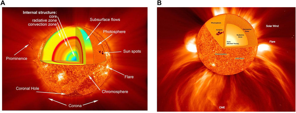
FIGURE 1. (A) The main regions of the Sun including the interior, surface (photosphere) and atmosphere (chromosphere and corona). Image Credits: NASA/Goddard. (B) Diagram adapted from SOHO/NASA representing the overall structure of the Sun including features such as CMEs, Flares, and the solar wind.
2.1 Solar Interior
Fueled by nuclear fusion processes, the core is the hottest and densest region of the Sun, with a temperature in excess of 107 K (Akasofu and Chapman, 1972). While the core accounts for less than 1% of the volume of the solar interior, it is responsible for generating the Sun’s vast supply of energy through fusing hydrogen into helium, which produces extraordinary amounts of heat, energy, and radiation. From the core, this radiation then travels through the radiative zone where it is constantly absorbed and re-emitted on its outward trajectory as the high density of this region results in a short mean free path for the emitted photons. Because of this absorption and re-emission process, the radiation can take tens to hundreds of thousands of years to leave the radiative zone (Russell et al., 2016).
Extending from the radiative zone to the photosphere (the optical surface of the Sun), the convective zone is a layer approximately 200,000 km thick dominated by plasma in the form of convective cells (Christensen-Dalsgaard et al., 1991; Stix, 2002). These cells form as a result of the temperature gradient between the base of the convective zone (at 2 million Kelvin) and its top (at 5,700 K), that moves plasma from the hotter core regions to the cooler regions in the photosphere. The convective zone plays an important role in the Sun’s behavior as it transports heat to the photosphere and drives the small-scale motion of the solar material (Moldwin, 2008). Figure 1A illustrates this internal structure of the Sun.
2.2 Solar Magnetic Field
Extending past the Kuiper Belt and shielding the Solar System from interstellar space, the Sun’s magnetic field is the largest magnetic structure in the Solar System. This field is likely generated by a dynamo process deep in the solar interior, but exactly where this process occurs remains unknown. Some models predict that the source region is located at the base of the convection zone, but others show that it could also lie deeper and involve the upper part of the radiative core (Solanki et al., 2006). However, no matter where the dynamo is precisely located, it forms magnetic field lines that the convecting plasma carries up through the convective zone as it moves from the hotter radiative zone boundary toward the cooler photosphere (Russell et al., 2016). Since the Sun is composed of a plasma, its fluid nature causes different latitudes on the Sun to rotate at different rates. This is known as “differential rotation” and, for example, at the Sun’s equator it takes approximately 25 days to complete a rotation while the poles take up to 30 days (Hathaway, 1994; Russell et al., 2016). In this system, energy is stored in magnetic structures in the form of twisted flux ropes, which emerge as visible energized systems once they break through the photosphere (Hathaway, 1994). Because of differential rotation, once a structure emerges on the surface of the Sun, depending on its orientation, one of the flux rope’s footprints may move at a different rate than the other. This causes energy to be loaded into the flux rope as its footprints are stretched and moved apart from one another as will be reviewed further in Section 2.4.1. In the dynamo process, the so-called Ω-effect, i.e., the winding of the poloidal field (contained in meridional planes) from differential rotation, produces a toroidal (i.e., longitudinal) field, and a twisting process (helical motions), called the α-effect, produces a poloidal field from the toroidal field (Schmitt, 1987; Charbonneau, 2010). More sophisticated models are needed to sufficiently describe the amplification of the toroidal magnetic field due to differential rotation (Schmitt, 1987; Charbonneau, 2010). Further discussion of solar dynamo modeling may be found in Charbonneau (2010) and Cameron et al. (2017).
The structure of the solar magnetic field and its properties undergo a remarkable transition through the Sun’s layers. The large scale toroidal fields produced by the Ω-effect have instabilities present that give rise to the formation of magnetic flux tubes (Leake and Arber, 2006). In the photosphere the field is highly filamented (Solanki et al., 2006) and the magnetic energy resides in these magnetic flux tubes. These structures concentrate the magnetic field and can be roughly described as bundles of nearly parallel field lines with a relatively sharp boundary, see Wiegelmann et al. (2014) and references therein. The flux tubes visible at the surface range from the very small and bright (magnetic elements) to the very large and dark (sunspots) (Solanki et al., 2006). The pressure exerted by the magnetic field leads to a considerable buoyancy that ensures that the magnetic field remains nearly vertical. Magnetic flux is believed to be transported to the surface by a mechanism called buoyancy, in which an isolated magnetic flux has a lower thermodynamic pressure than its gaseous surroundings, and as a result rises due to this magnetically-induced buoyancy (Acheson, 1979). This process is known as flux emergence and the emerging fields evolve to form complex structures on the Sun such as coronal loops and prominences. Flux emergence also influences eruptive events in the corona, or upper atmosphere of the Sun (Leake and Arber, 2006). Through the photosphere, magnetic buoyancy instability causes the magnetic field to expand into the atmosphere of the Sun and into the corona. This expansion is driven by the emergence of magnetic flux via magnetic buoyancy from the convective zone into the stable layers of the photosphere and results in a horizontal expansion of the magnetic field. This expansion results in the formation of a magnetic layer that is unstable to the magnetic buoyancy instability, which drives the magnetic field into the above atmosphere (Matsumoto and Shibata, 1992; Leake and Arber, 2006).
One measure of the effect that the magnetic field has on the plasma is called the plasma beta (β), defined as the ratio of the dynamic pressure to the plasma pressure:1
where p is the gas pressure, B is the magnetic field strength, and μ0 is the permeability of free space. For the magnetic flux tubes, the plasma beta ranges between 0.2–0.4, which means that, locally, the magnetic field dominates the bulk motions. Moving into the higher atmosphere, both the gas and the field strength decrease exponentially, in a way that the plasma β remains mostly constant (Solanki et al., 2006).
A useful type of image used to study the Sun’s magnetic field is called a magnetogram. A magnetogram, produced by an instrument called a magnetograph, takes advantage of the Zeeman effect by using emission-line splitting to measure the line-of-sight components of the magnetic fields at the surface of the Sun. Magnetograms are extremely useful for producing modeled solar magnetic fields, as they allow for the reconstruction of the model field’s orientation using the polarities given by the magnetogram, see e.g., Riley et al. (2006) and references therein. Figure 2 shows an example of a magnetogram from Solar Dynamics Observatory (SDO) spacecraft using Helioseismic and Magnetic Imager (HMI) instrument (Scherrer et al., 2011).
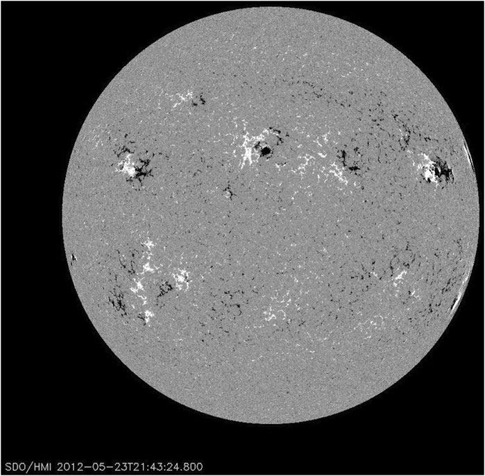
FIGURE 2. Magnetograms show maps of the magnetic field on the Sun’s surface, with black showing magnetic field lines pointing away from Earth, and white showing magnetic field lines coming toward Earth. Image Credits: NASA/SDO/Goddard.
2.3 Outer Layers of the Sun
Magnetic maps such as the one shown in Figure 2 are attributed to the Sun’s optical surface called the photosphere, which is a thin (about 1,000 km thick) layer that is responsible for all of the visible light that we receive from the Sun (Gray, 2005). It is also much cooler than the solar interior, having a temperature of 6000 K. The photosphere is considered to be the optical surface of the Sun as it sits at the transition where gaseous layers change from completely opaque to transparent. On the photosphere we can see sunspots, which are regions where magnetic flux ropes come through the solar surface as previously discussed (Russell et al., 2016). This magnetic field inhibits convection, making the sunspots cooler and thus appear darker than the rest of the photosphere as seen in Figure 1A. Additionally, sunspots often form in pairs as they are byproducts of the flux rope emergence. The sunspots’ brightness and temperature are functions of spatial position. This is due to the magnetic field structure and properties changing with height. A more thorough discussion of this change in properties may be found in Borrero and Ichimoto (2011). Magnetic flux tubes are part of this structure, storing most of the magnetic energy in the sunspots. Surrounding sunspots are areas called active regions which result from magnetic field instabilities created near the sunspots, see Solanki (2003). Normally active regions have magnetic field configurations that are bipolar, including both positive and negative polarity, but more complex active regions may be comprised of several of these configurations that are in close proximity (van Driel-Gesztelyi and Green, 2015). They are widely understood to form via magnetic flux tubes originated from the toroidal magnetic field which then undergo magnetic buoyancy through the photosphere and into the solar atmosphere (Zwaan, 1987). The magnetic flux that make up a given active region originates from the convective zone, and causes the active region to grow from the inside outwards.
Because the photosphere is also on top of the convective zone, its surface is made up of convective cells called granules, which are cells of plasma with hot rising material in the center and cooler falling plasma on the edges as expressed in (Wiegelmann et al., 2014; Russell et al., 2016). This creates the “granulated” look of the Sun’s surface as seen in Figures 1A,B.
Sitting above the photosphere is the solar atmosphere, which is separated into two sections: a lower region called the chromosphere and an upper region known as the corona. The chromosphere extends to 2000 km above the photosphere, has a temperature of about 104 K (Stix, 2002), and appears visually as a reddish layer above the photosphere. This region contains several main solar structures including filaments and prominences (Russell et al., 2016). Filaments are dark lines that appear on the surface of the Sun (normally above sunspots) and consist of large arcs of plasma lifted from the surface by magnetic flux ropes. This cools the material and makes it appear darker than the surrounding chromosphere and photosphere and allows us to view these structures in the H-alpha wavelength, or the red emission line of hydrogen (Shine and Linsky, 1974). When seen on the limb of the Sun, filaments are instead known as prominences, as seen in Figure 1. These prominences are seen as plasma arcs profiled against the solar corona and interplanetary space, instead of the brighter surface of the Sun. In addition to these more prominent structures, there are also plages and the chromospheric network. Plages are bright concentrations of magnetic field in the chromosphere which can be seen in H-alpha, while the chromospheric network defines the bright outlines of large scale granules that are generated by the convection of plasma on their boundaries and can be seen in H-alpha and in calcium’s ultraviolet line—Ca II K (Shine and Linsky, 1974).
Lastly, above both the photosphere and chromosphere, we encounter the corona, or the upper atmosphere of the Sun. Interestingly, the corona is also the hottest region of the Sun’s atmosphere, having temperatures above one million kelvin—orders of magnitude hotter than the photosphere. The corona’s intensely hot plasma is mostly optically thin and emits mainly in the following regions of the electromagnetic spectrum: X-ray (5–50 Å), soft X-ray (50–150 Å), extreme ultra-violet (EUV, 150–900 Å) and far ultra-violet (UV, 900–2000 Å) (Zanna and Mason, 2018). Once viewed, the corona can appear spattered, presenting a mixed-polarity magnetic field, where the small bipolar regions give rise to bright points in the EUV and X-ray wavelengths. The enhanced magnetic field in these regions corresponds to bright active region forms, with a multitude of extended loop structures. The other large-scale features are coronal holes, which appear as darker areas in EUV and soft X-Ray images, corresponding to clusters of open magnetic field (poloidal field) lines at the photospheric level (Cranmer et al., 2017; Zanna and Mason, 2018). These open field lines allow solar material to easily escape from the Sun’s surface, leading to coronal holes having lower density and temperature than the rest of the corona. These regions are known as coronal “holes” as the magnetic field only connects to the Sun at one end, leaving regions or “holes” of open magnetic field lines. Despite the importance of the corona to the solar environment and the larger heliosphere, it is difficult to directly and reliably measure the magnetic field in the corona. Due to this difficulty, it has been necessary to rely instead on models of the coronal and interplanetary magnetic field (Gombosi et al., 2018). This being said, the recent study by Yang et al. has indicated success in using Coronal Multi-channel Polarimeter (CoMP) to construct a global map of the visible coronal magnetic field (Yang et al., 2020). Further discussion about the solar corona and its features can be found in the Zanna and Mason (2018) review or papers such as Cranmer et al. (2017) and Richardson (2018).
Regarding the magnetic field in the Sun’s atmosphere, its strength decreases exponentially in the chromosphere and even more rapidly in the corona (Solanki et al., 2006). As a consequence of this and other conditions, the magnetic Lorentz force cannot be balanced by any other force, so the coronal magnetic field has to arrange itself into a force-free configuration, which is homogeneous in strength but not in direction, resulting in the field’s inclination at all heights in the corona. Since currently no measurements of the magnetic field in the solar corona are available, it is necessary to use measurements such as full disk magnetograms over a solar rotation in order to measure the surface magnetic field distribution, and then provide this as input to simulate realistic coronal and interplanetary magnetic field models (Gombosi et al., 2018). At r ≳ 2 − 3R⊙, most of the remaining field lines are “open”, i.e., they reach out into the heliosphere as will be discussed below.
2.4 Eruptive Events in the Corona
2.4.1 Magnetic Reconnection and the Storage of Energy
Perhaps the single most important concept in space weather is magnetic reconnection. This process provides the means by which magnetic energy can be converted into kinetic energy (Sweet, 1958; Parker, 1963), making it the fundamental driving force behind most space weather related events (Yamada et al., 2010). Note that magnetic reconnection is a complex process as it involves both micro (kinetic) scales and macro (magnetohydrodynamic-MHD) scales, making it a multiscale process that details the reconfiguration of magnetic field lines and the resulting release of energy (Zweibel and Yamada, 2016). While the Sun is full of magnetic energy, the corona is effectively superconductive, so its magnetic energy can only be dissipated through magnetic reconnection, which unlocks physical processes such as plasma acceleration, shocks, and charged particle events that are fundamental to understanding space weather effects on Earth.
The physical process of reconnection is depicted in Figure 3 where the merging of opposing magnetic field lines, creates a magnetic instability such that the field lines connect. While the release of energy happens in the Sun’s corona, the storing and buildup of energy occurs within the solar interior (Holman, 2012). As noted from the previous section, the system is energized by the subsurface flows in the lower atmosphere of the Sun, specifically the differential rotation of the Sun’s plasma at different latitudes, as well as meridional, moving north and south, flows at different longitudes. This difference in the flow of plasma causes imperfections or “kinks” in the Sun’s magnetic field as it is carried along with the flow of plasma (Yamada et al., 2010). These kinks create magnetic flux ropes which store energy on the surface of the Sun. Janvier et al. (2015) and Leake et al. (2013) provide a more detailed description of the forming of twisted flux ropes in the corona.
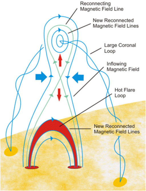
FIGURE 3. Idealized model of magnetic reconnection on the solar surface. The merging of opposing magnetic field lines created a magnetic instability, causing the field lines to connect. In this model, arcs of field lines connect two sunspots which lie below the chromospheric footprints of the magnetic flux rope. During reconnection, the new reconnected magnetic field lines separate as the top loop expands upward while bottom loop collapses inward. This process forms a current sheet, causes energy release, and ejects plasma upward along the field line. Image Credit: NASA.
Once enough energy is stored, the magnetic loop is deformed to the point that some of its field lines reconnect with another set of field lines. This causes an instability that allows the magnetic reconnection to release energy over a short time period, causing magnetic energy to be partially converted into thermal energy (Green et al., 2018). As seen in Figure 3, this may occur when arcs of field lines (such as in flux ropes) connect two sunspots, representing the footprints of the flux rope. During magnetic reconnection, the chromospheric footprints of the flux rope separate, as the top loop in Figure 3 expands upward (Georgoulis et al., 2019). The loops then collapse inward and reconnect, forming a current sheet and causing the acceleration and propagation of charged particles (Dungey, 1953). Note that while the current sheets are expected to be highly fragmented and dynamic, their spatial resolutions are very low, and are therefore difficult to image (Klein and Dalla, 2017). Multiple current sheets can be formed in a magnetic loop that is twisted by the motion of the chromospheric footprints (Georgoulis et al., 2019). Magnetic reconnection forces the top loop upwards, causing energy release and ejecting plasma upward along the field line. It is also important to note that magnetic reconnection on the Sun can occur with an open structure or with another closed structure.
In all, the loading of energy into the magnetic field forms some of the more recognizable solar structures including sunspots, active regions, filaments, prominences, as well as more violent and eruptive events such as coronal mass ejections (CMEs), solar flares, and solar energetic particle (SEP) events. All of these events, however, are created in the same fundamental manner as described by (Sweet, 1958; Parker, 1963; Green et al., 2018). This process is a part of the aforementioned reconfiguration of the Sun’s magnetic field, where the field topology can change through magnetic reconnection. Once sunspots move apart from one another, driven by differential rotation or meridional flows, the field lines are stretched, eventually deforming the magnetic topology leading to magnetic reconnection (Kulsrud, 1998). This breaks off a portion of the field, accelerating it outward (Green et al., 2018). During magnetic reconnection, the released energy from the magnetic field can take the form of a solar flare, whose energy represents a tremendous outburst of electromagnetic radiation in many different wavelengths. Additionally, the accelerated portion of the filament (or prominence) can drag plasma with it out from the chromosphere into the corona and into interplanetary space. When this occurs, the resulting outburst of magnetic field and plasma is a coronal mass ejection or CME (Georgoulis et al., 2019). Solar energetic particles (SEPs) accompany both flares and CMEs, and represent high energy particles that are also accelerated during these events. Because they are charged, they tend to follow magnetic field lines and are thus essentially tied to the Parker spiral pattern. Through this connection, SEPs that affect Earth mainly originate from the western hemisphere of the Sun (Laitinen and Dalla, 2019).
2.4.2 Coronal Mass Ejections
Magnetic reconnection events in the solar corona can cause a large-scale explosive release of energy and mass, in particular, via the so-called “magnetic breakout”—a positive-feedback mechanism between filament ejection and reconnection (Antiochos et al., 1999; Wyper et al., 2017).
One classic example of a solar eruptive event is a coronal mass ejection (CME). Coronal mass ejections primarily occur in active regions on the Sun, where there are strong magnetic field lines and closed-field structures. Several mechanisms influence the course towards an eruption resulting in a coronal mass ejection; these mechanisms are often called triggers and drivers of an eruption (Georgoulis et al., 2019). Examples of triggers include magnetic reconnection and examples of drivers include the shearing or twisting of the magnetic flux ropes comprising the magnetic loops of an active region. Both triggers and drivers influence the magnetic loop configurations by pushing the idealized loop model shown in Figure 3 to a critical point where loss of stability occurs, leading to an eruption of solar material as the supported magnetic structure is severed from its connection to the Sun and is accelerated outward (Forbes, 2000).
Once this mass of plasma and magnetic field accelerates outward from the Sun, its structure becomes apparent with a bright core representing the filament/prominence in the active region of concern, a dark, inner cavity where the magnetic flux rope of the magnetic loops resides, and a bright outer loop containing the coronal material and streamer (Low, 1996). This structure, and its evolution, can be clearly seen in Figure 4, which shows a CME’s propagation away from the Sun. After a CME erupts, we can derive its speed by using multiple measurements over time from several coronagraphs in orbit around the Sun. Examples include the coronagraphs aboard the twin spacecraft STEREO (Solar Terrestrial Relations Observatory) A and STEREO B, which orbit around the Sun at different solar longitudes, allowing for the reconstruction of CME propagation based on multiple viewing angles (Mierla et al., 2008). The general propagation profile of a CME has it beginning as a slow rise moving at about tens of kilometers in the timescale of minutes. The CME then rapidly accelerates a few solar radii in timescales of hours before finally propagating constantly into interplanetary space and through the heliosphere (Georgoulis et al., 2019). The CME carries with it a magnetic shock and sheath region, along with shocked plasma that is heated, dense, and turbulent. Figure 4 shows the 60 min evolution of a CME imaged by the Large Angle and Spectrometric COronagraph (LASCO)/C2 coronagraph instrument aboard of the Solar and Heliospheric Observatory (SOHO) spacecraft, combined with matching data from the SDO/AIA.
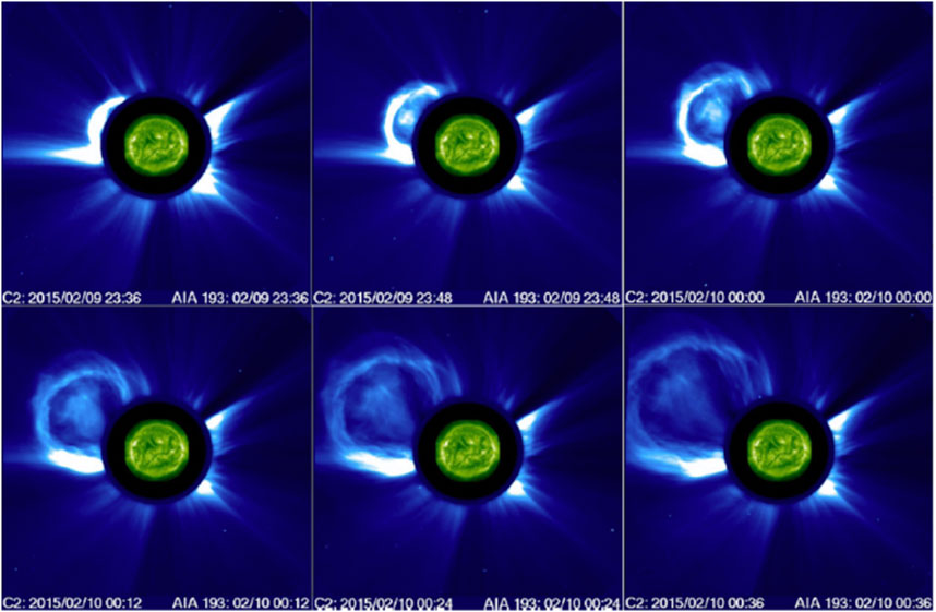
FIGURE 4. 60 min propagation of a CME as imaged by the LASCO/C2 coronagraph aboard the SOHO spacecraft. Notice the idealized structure present in the image of a bright inner core, a dark cavity region, and a bright outer loop (Georgoulis et al., 2019).
It is worth noting that CMEs can happen with or without a flare present. In fact, Gosling (1993) argued that solar flares do not play a fundamental role in producing CMEs, and even suggests that more than 80% of all observed CMEs are not associated with large flares. Of the CMEs that are associated with solar flares, Simnett and Harrison (1985) and Wagner and MacQueen (1983) showed that CME trajectories can be frequently extrapolated to a time prior to the start of the flare, suggesting that CMEs often initiate prior to the onset of a flare. The scope of this paper does not allow for a comprehensive review of coronal mass ejections; however see e.g., Forbes (2000) for more details.
2.4.3 Solar Flares
Another classic example of magnetic reconnection’s impact on the solar environment are solar flares, which represent impulsive and intense bursts of radiation. Giovanelli (1946, 1947) first demonstrated that solar flares are an electromagnetic process of energy conversion (Bai and Sturrock, 1989). Typical flares last from seconds to hours and emit radiation at mostly short wavelengths; however, large flares often produce electromagnetic radiation at all observable wavelengths including the visible spectrum, in which case the flare is known as a “white light flare” (Russell et al., 2016). Figure 5A shows a solar flare in different wavelengths of the Extreme Ultraviolet (EUV) spectra. Solar flares occur when magnetic flux emerges from the lower regions of the Sun onto its surface and form new active regions, and are believed to be at least partially responsible for heating the Sun’s corona (Solanki et al., 2006). The first observation of a solar flare was a white light flare observed in September of 1859 in an event that is now dubbed the “Carrington Event”, which heralded the arrival of one of the largest space weather storms in modern history.
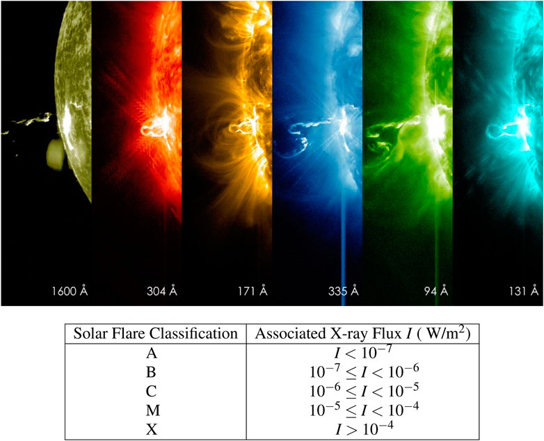
FIGURE 5. Top panel: This image illustrates a solar flare seen in different wavelengths of ultraviolet light, from 1,600 Å on the left to 94 Å and 131 Å on the right. Note that since flares are EM radiation events, they are visible in multiple wavelengths as depicted in the figure above. Image Credit: NASA/SDO. Bottom panel: Description of solar flare classes where the definition of the flare classes is based upon their peak flux in X-rays of 1–8 Å (Discola Junior, 2019).
Like CMEs, solar flares mostly occur in active regions, since these regions contain strong, complex magnetic fields and magnetic loops of hot and dense plasma (Janvier et al., 2015). Solar flares are also, as previously discussed, a byproduct of the complex reconfiguration of the magnetic field and the release of energy via magnetic reconnection, see e.g., Cliver et al. (1986). The complexity of the overall system has naturally lead to rigorous debate about which specific mechanisms are primarily responsible for the sudden eruption of energy seen in solar flares, as well as which energy conversion processes are most important to cause this energy release; Bai and Sturrock (1989) reviews this topic in greater detail.
Solar flares are classified (by energy) into several categories: A, B, C, M, and X, with A being the least intense and X being the most intense (Janvier et al., 2015). Each category has nine subdivisions ranging from, e.g., C1 to C9, M1 to M9, and X1 to X9, and is subdivided based on X-ray measurements from the Geostationary Orbiting Environmental Satellites (GOES) (Bai and Sturrock, 1989). The table in Figure 5 lists different classifications of solar flares, along with their associated X-ray fluxes.
Solar flares can unfold as a confined or eruptive process. In confined flares, the magnetic field elements are contained into flare loops, and are accompanied by accelerated particles (Pallavicini et al., 1977). Simulations have shown that in a confined flare, as new flux emerges, it pressures against overlying field structures, which leads to the formation of a current density layer (Janvier et al., 2015). This current then increases until a threshold is reached and a micro-instability is triggered. This micro-instability increases the local resistivity of the plasma, which rapidly dissipates the current (Janvier et al., 2015). Confined flares are generally impulsive in time and compact in space, and the flare loops contain most of the energy. Eruptive flares, on the contrary, generally extend to a large volume of the corona and lead to the ejection of solar material in the form of coronal mass ejections (Pallavicini et al., 1977). Eruptive flares are generally associated with long duration events, while confined flares typically have a much shorter time scale (Bai and Sturrock, 1989).
When studying flares, we can note that their peak emissions at each wavelength do not happen at the same time. Therefore, if we look into a wide range of the electromagnetic spectrum, we can see the time evolution of each flare as explained in the in-depth review conducted by Janvier et al. (2015).
2.5 Solar Cycle
The Sun transitions through periods of high and low solar activity, which is called the solar cycle. This cycle lasts approximately 11 years, and can be characterized by times of solar maxima and solar minima, see Figure 6. Additionally, the magnetic poles of the Sun are inverted every cycle, resulting in a 22 years complete cycle. During solar maximum, the Sun has a larger number of active regions, whereas in solar minimum, the Sun has a smaller number of active regions, this process has been reviewed by Zwaan (1985, 1992). These active regions are mechanisms through which particles can be accelerated, such as solar flare-related coronal jets (Russell et al., 2016). The solar cycle is a consequence of the reconfiguration of Sun’s magnetic field over time, as previously described in Section 2.4.1. Magnetic activity can be directly correlated to the number of sunspots present on the photosphere. Because of this, the number of sunspots observed at a given time can be a valuable measurement of solar activity, as this number is well-correlated to characteristics such as the total surface magnetic flux or the total solar radio flux (Solanki et al., 2006). Figure 6 shows a depiction of the solar cycle. Note that solar phenomena are correlated with the solar cycle, such as solar flares and CMEs, as they occur more frequently in times of solar maximum, and occur less frequently in times of solar minimum.
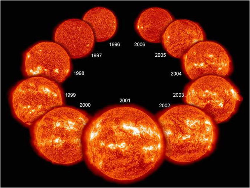
FIGURE 6. A depiction of the solar cycle where, starting from a solar minimum in 1996, the image cycles through to solar maximum in 2001, then back to solar minimum in 2006, showing a full 11 years cycle. Note how the Sun shows little activity during solar minimum with very few active regions, while, during solar maximum various active regions, prominences, and filaments can be seen. Image Credit: NASA.
3 The Heliosphere
Expanding from the Sun out to the boundary of interstellar space, the heliosphere represents a massive bubble carved out of the interstellar medium by the Sun’s magnetic field and solar wind. Inside the heliosphere’s protective bubble, material and magnetic field outflow from the Sun dominates, resulting in the transfer of energized solar plasma into interplanetary space and creating the basis for energy transport in the space weather system.
3.1 The Solar Wind
The solar wind represents the continual outflow of charged particles and magnetic field from the Sun’s upper atmosphere into interplanetary space. This outflow is generated through thermal pressure gradients as the plasma in the Sun’s atmosphere is heated to such a point that the gas pressure difference between interplanetary space and the solar corona generates pressure gradient forces strong enough to overcome the Sun’s gravitational pull (Cranmer et al., 2017).
Because the solar wind is created from the Sun’s upper atmosphere, its composition reflects that of the Sun as a whole, being comprised of a majority of hydrogen and helium. Specifically, the solar wind is 96% protons, 4% alpha particles, and contains trace amounts of carbon and heavier elements (Wurz, 2005).
When plasma escapes from the solar atmosphere, it expands outward into a spiral formation known as the Parker Spiral. This distribution is created as solar wind source regions steadily change their position due to the Sun’s rotation (Russell et al., 2016). Thus, even though these source regions eject material on a radial path away from the solar atmosphere, the rotation of the source regions themselves results in a spiral distribution for the solar wind as shown in Figure 8A.
Because the solar wind is comprised of highly conductive plasma, it also carries the Sun’s magnetic field as it moves forward due to Alfvén’s frozen-in flux theorem ensuring that the magnetic flux is “frozen” into the plasma (Roberts, 2007). This leads to the formation of spiral magnetic field lines. The tightness with which the magnetic field lines are wound depends on the speed of the solar wind, with slower winds creating lines that are wound tighter and faster winds causing lines to be more loosely wound.
The spiral magnetic field lines in the Parker Spiral follow the relation
where V is the solar wind speed, r is the heliocentric distance, Ω is the solar angular velocity, θ and ϕ are respectively the helio-altitude and helio-longitude of the observer, and r0 and ϕ0 are the heliocentric distance and helio-longitude of the initial plasma position at the Sun (Richardson, 2018).
The expansion of the Sun’s large-scale dipole magnetic field out into the heliosphere leads to open, oppositely directed magnetic field lines approaching one another along the heliosphere’s magnetic equator (Smith, 2001). To balance these oppositely directed magnetic field lines, the heliospheric current sheet or HCS is created and divides the Sun’s magnetic field where its polarity changes between north and south (Kahler, 2003).
The solar wind also exhibits structure on a range of spatial and temporal scales. Most fundamentally, it is observed to be bi-modal in nature, having “fast” and “slow” streams (Habbal et al., 1997). “Fast” wind originates from coronal magnetic regions where the field is only connected to the Sun at one end, i.e., regions of “open” field lines known as coronal holes, as previously mentioned in Section 2.3 and shown in Figure 7, where the extra escaping material from these regions is responsible for the creation of high-speed solar wind streams. On the other hand, “slow” wind appears to come from a wide range of sources, including streamers, pseudo-streamers, coronal loops, active regions, and coronal hole boundaries (Cranmer et al., 2017). Coronal holes that last for multiple solar rotations are the source of what are known as corotating interaction regions (CIRs), where the “fast” solar wind that is released from the coronal hole interacts with “slow” wind (Richardson, 2018).
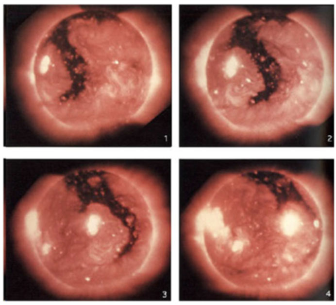
FIGURE 7. Four images of soft X-ray observations of a coronal hole (dark region) extending from the north pole to the equator of the Sun. These images were taken 2 days apart (Richardson, 2018). These images were distributed under the https://creativecommons.org/licenses/by/2.0/legalcode Creative Commons Attribution 2.0 International License.
The interaction of fast and slow wind leads to patterns of solar wind compression and expansion, forming stream interaction regions (SIRs). Because the plasma is “frozen in” to the magnetic field, these streams cannot mix and are a common source of interplanetary shocks, though both SIRs and CIRs can occur independently of shock formation. During the formation of SIRs, the fast wind interacts with and deflects the slower wind to the west while the slower wind deflects the faster wind to the east. Additionally, the lack of mixing allows the two streams to be distinguished by their ion composition, i.e., the “slow” wind is denser.
3.2 Shocks, ICMEs, and SEPs
In addition to its base outflow of solar material from the solar atmosphere, the solar wind may exhibit structure in the form of shocks. These shocks occur in the collisionless plasma of the solar wind from the pileup of magnetic field lines (Pizzo, 1978). Shocks may occur in front of solar drivers near the Sun, with shocks farther out into the heliosphere generally driven by CMEs and SIRS [e.g., Guo et al. (2021)].
CMEs as they move out into the interplanetary medium are known as interplanetary coronal mass ejections (ICMEs) and drive shocks as they inject fast moving plasma and magnetic field lines into the interplanetary medium. Specifically, interplanetary shocks can occur when an ICME is sufficiently faster than the preceding solar wind, resulting in a shock wave developing ahead of the ICME (Kilpua et al., 2017). See Figure 8B for an example of an ICME’s outward propagation and its resulting interplanetary shock.
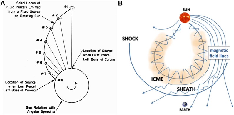
FIGURE 8. (A) Depiction from Russell et al. (2016) of the formation of the Parker spiral by the Sun’s rotation causing parcels of radially emitted plasma to be released from the Sun at differing locations because of the ever-changing orientation of the emission region on the Sun’s surface. (B) Diagram of an ICME as it moves through interplanetary space (Kilpua et al., 2017). This image was distributed under the https://creativecommons.org/licenses/by/4.0/legalcode Creative Commons Attribution 2.0 International License. Note the spiral magnetic field lines created because of the Parker spiral pattern explained in (A).
Interplanetary shocks can trigger geomagnetic storms when they interact with Earth’s magnetosphere (Lakhina and Tsurutani, 2016). Additionally, CME-driven shocks have an important role in the acceleration of solar energetic particles. An SEP event is defined as the direct enhancement of the fluxes of protons, electrons, and other heavy ions and energies well above the thermal energy in the Sun’s corona, which is typically hundreds of electron volts (Russell et al., 2016). These events can reach up to GeV levels in energy and can last anywhere from a few hours to several days (Klein and Dalla, 2017). GeV SEP events are significant in regards to their impact on Earth as they produce ground level enhancements, which are interpreted as enhancements in the cosmic ray intensity as measured by detectors on Earth (Plainaki et al., 2014) and represent hazardous conditions for satellites as well as manned mission (e.g., Mishev and Usoskin, 2020).
SEP events are often divided into impulsive or “weak”, and gradual or “strong” events (Reames, 1999). Impulsive SEP events are short duration (usually less than 1 day), have modest fluxes (meaning that they are generally low in intensity), and occur frequently (up to 1,000 per year) during periods of high solar activity. Impulsive SEP events usually have rapid onset and decay times, and generally only last a few hours. Gradual SEP events are long in duration (usually several days), and are high in intensity. They are generally rarer, as there are usually only about a few dozen per year (Klein and Dalla, 2017).
Energetic particles in impulsive events are thought to be accelerated close to the Sun by the rapid energy release in the impulsive phase of a solar flare and by the consequent strong wave activity. The main ICME-related shock acceleration mechanism is diffusive acceleration mechanism (DSA) (Hu et al., 2017). During the acceleration process the accelerated particles must cross the shock several times, gradually gaining energy until they escape from the shock region (Klein and Dalla, 2017). On the other hand, energetic particles in gradual events are thought to be accelerated in CME-driven shocked primarily through the diffusive shock acceleration mechanism.
SEPs are accelerated in two main categories: first via magnetic reconnection and turbulence in active regions usually generated by solar flares, and second via large-scale CME-driven shocks (Kilpua et al., 2017). The distinction between these types of events can be difficult and the origin of accelerated SEPs continues to be highly debated (Cliver, 2016), as solar flares and CMEs occur nearly simultaneously when the same, or nearby, active regions erupt. In addition, properties of gradual SEP events are influenced by several processes [e.g., Desai and Giacalone (2016)] such as: the origin and variability of the suprathermal seed populations; the shock geometry and background magnetic field; the injection threshold and efficiency of the shock acceleration mechanisms; the presence of multiple, interacting CMEs; the waves and turbulence present near the shock and in the interplanetary medium; and scattering conditions during transport in interplanetary space.
Finally, it is known that particles are accelerated during solar flares, when the chromosphere is heated by energy deposition during the flare (Jeffrey et al., 2019). This source is generally interpreted as a signature of energy release near or above the loop top, which heats the plasma in the coronal loop and accelerates electrons that can escape from the primary acceleration site as beams. Because of their high energy they do not interact much with the coronal plasma that have been diluted, and instead release energy at the “chromospheric footprints” of the loops (Klein and Dalla, 2017).
3.3 Heliospheric Structures
As previously observed, the Sun’s magnetic field and solar wind creates a bubble-like region of plasma around the solar system called the heliosphere. The heliosphere mimics the shape of the magnetosphere in many ways: it is a circumsolar structure that has a hemisphere shape in one direction due to compression by the interstellar wind and extends in a long comet-like tail behind it (Kilpua et al., 2017).
The heliosphere has a layered structure, as shown in Figure 9: when the solar wind leaves the Sun, it travels at supersonic speeds until it reaches the termination shock, whereupon it begins to slow and compress as it expands out into the interstellar medium. This compression causes the particles in the solar wind to heat up (Fahr, 2004). The termination shock starts diverting the solar wind plasma down to the tail of the heliosphere, beginning the formation of the tail. The region of shocked, heated solar wind plasma beyond the termination shock is known as the heliosheath (Burlaga et al., 2005).
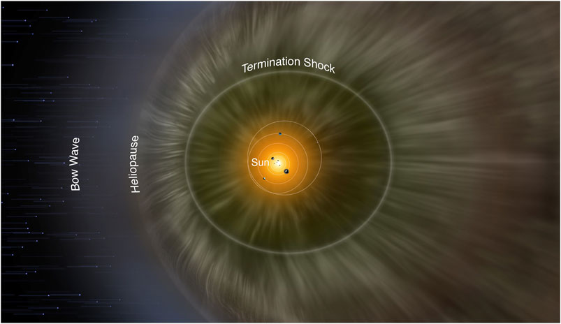
FIGURE 9. A schematic of the heliosphere’s structure depicting the termination shock and heliopause. Image Credits: NASA/IBEX/Adler Planetarium.
Past the heliosheath, believed to be around 30–40% more distant than the shock, is the heliopause as depicted in Figure 9. The heliopause is the dividing line between solar wind plasma and interstellar plasma (the solar wind and the interstellar wind) (Fahr, 2004). Voyager 1 crossed the termination shock at 94 astronomical units (AU) in 2004 and is believed to have crossed the heliopause in 2012 at a distance of 121 AU (Gurnett et al., 2013).
As CMEs and fast solar wind streams can overtake the regular solar wind on its path towards the heliopause, they create compressed regions of plasma and magnetic field lines called merged interaction regions (MIRs) (Fahr, 2004). Rarefactions then form behind the MIRs where plasma has been cleared out. As the magnetic field in these regions is higher, they help block cosmic rays from entering the solar system. But while the solar wind defines the boundaries and structure of the heliosphere (as the boundaries are created where the pressure of the solar wind balances with that of the interstellar medium), it varies with the solar cycle (Bazilevskaya et al., 2015). During solar maxima, there are relatively few high-speed streams, and the average speed of the solar wind is lower. This variability, along with the irregular occurrence of CMEs and high-speed streams throughout the solar cycle, causes the boundaries of the heliosphere to oscillate (Fahr, 2004).
4 The Earth’s Magnetosphere
After flowing unobstructed through the solar system, the solar wind first encounters resistance when it comes into contact with planetary magnetic fields. According to Pulkkinen (2007), “a magnetosphere is a cavity in the solar wind flow formed by the interaction of the solar wind and interplanetary magnetic field (IMF) with the intrinsic magnetic field or ionized upper atmosphere of a planetary body.” Thus, the Earth’s magnetosphere is the region where Earth’s magnetic field is dominant, and is subdivided into the magnetosheath, magnetopause, magnetotail, plasmasphere, and radiation belts, as shown in Figure 10. These divisions are based on the magnetic field lines and plasma characteristics, such as its origin, density and energy levels. This magnetic field protects us from some of the heliosphere’s harshest conditions and the constant flow of charged particles via the solar wind. Events on the Sun leading to large perturbations in the magnetosphere are called geoeffective.
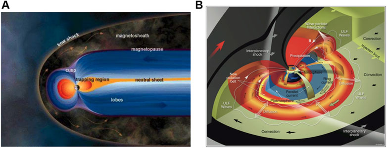
FIGURE 10. (A) The Earth’s outer magnetosphere with the bow shock, magnetosheath, magnetopause, tail lobes, and tail current sheet (also called the neutral sheet) shown. The Sun is assumed to be on the left of the image, thus the solar wind compresses the dayside (or sunward) magnetosphere, while it stretches the nightside magnetosphere into the tail region. Note the cusp regions of weaker magnetic field strength that lead directly into the Earth’s upper atmosphere at high latitudes (Pulkkinen, 2007). This image was distributed under the https://creativecommons.org/licenses/by/4.0/legalcode Creative Commons Attribution 2.0 International License. (B) Representation of the inner magnetosphere depicting the ring current, radiation belts, and plasmasphere (Mauk et al., 2013). This image was distributed under the https://creativecommons.org/licenses/by/4.0/legalcode Creative Commons Attribution 2.0 International License.
4.1 The Earth’s Magnetic Field
Earth’s intrinsic magnetic field is created deep in its hot, partially liquid iron-nickel core by a self-exciting dynamo process thought to form through the movement of east-west aligned flows in the molten, conducting outer core (Gubbins, 1974; Glatzmaier and Roberts, 1995). In addition to this dynamo process, there is a static field produced by rocks carrying magnetized minerals in the Earth’s mantle. This additional field is called the lithospheric field and is generally significantly smaller than the core’s dynamo magnetic field which makes up 95% of the magnetic field strength at the Earth’s surface (Cranmer et al., 2017; Mandea and Chambodut, 2020).
The Earth radius (Re ≈ 6,380 km) is a natural length scale for the magnetosphere. Near the Earth, up to 3 to 4 Re, the field can be approximated with the field of a dipole; specifically, the field is characterized as being about 90% dipole, with a magnetic dipole moment of 7.65 × 1025 erg/G, resulting in a magnetic field strength at the surface of about 30,000 nT at the equator and 60,000 nT near the poles (Stacey and Davis, 2008). The geomagnetic field is oriented so that a magnetic S pole is near the geographic north pole, and a magnetic N pole near the geographic south pole. The geomagnetic field is tilted at about 11° with respect to the rotation axis. However, at larger distances, the effects of the solar wind causes significant deviations from the dipole. As the magnetic field acts like a tilted dipole, the regions where the field lines diverge between flowing toward the dayside magnetosphere and the tail are called the cusps, as seen in Figure 10A. The cusp regions also mark where the magnetic field is at its minimum, allowing solar wind plasma to reach into the Earth’s upper atmosphere (Ganushkina et al., 2018).
The orientation of the geomagnetic field reverses itself at irregular intervals, the last such geomagnetic reversal having occurred about 780,000 years ago. The mechanism responsible for these reversals remains largely unknown, although the geological record shows that the reversals happen relatively quickly relative to geological times scales of 105–106 years [Jacobs (1995), Singer et al. (2019)].
4.2 The Outer Magnetosphere
When the magnetised and supersonic solar wind first encounters the obstacle of Earth’s magnetosphere, a standing shock wave is formed, termed the bow shock (Milan et al., 2017) as shown in Figure 10A. After crossing this boundary, the solar wind plasma becomes shocked, or heated and slowed, and is diverted around the magnetosphere due to the solar wind’s frozen-in magnetic field resisting the Earth’s magnetic field. The plasma then resides in the magnetosheath, which is a region of turbulent plasma that is much denser, hotter and slower than the solar wind (Akasofu and Chapman, 1972).
Separating the magnetosphere’s stronger magnetic field from the weaker magnetosheath (the solar wind’s field), the magnetopause represents the region of pressure balance between the solar wind and the steady presence of Earth’s magnetic field, given by the following approximate condition (Kanani et al., 2010; Russell et al., 2016; Ganushkina et al., 2018):
where ρsw is the solar wind’s density, vsw is the solar wind’s velocity, and BE is Earth’s magnetic field strength. The left-hand side of this equation represents the kinetic pressure of the solar wind, and the right-hand side represents the magnetic pressure of the Earth’s magnetic field. The solar wind’s kinetic pressure then compresses this magnetic field on the dayside, as seen in Figure 10A, but, as the solar wind is dynamic, the location of the magnetopause changes with solar wind conditions causing the boundary to essentially “breathe” in and out as the solar wind lulls and surges. From the pressure balance Eq. 3, one finds the magnetopause sub-solar standoff distance to be given by Anderson (2004)
During typical solar wind drivers the average conditions are as follows: ρsw = nswmp, nsw ∼ 7 cm−3, vsw ∼ 400 km/s, and equatorial geomagnetic field strength 30, 000 nT. During these times, the magnetopause is approximately 10 Re upstream from Earth, but when the solar wind is particularly strong, such as during geomagnetic storm driving conditions, it can compress inside the geostationary orbit, reducing the stand-off distance to less than 6.6 Re (Pulkkinen, 2007). Thus the magnetopause regulates the transfer of mass and energy from the solar wind into the inner magnetosphere and also contains a current structure which supports the magnetopause.
Because of the pressure that the solar wind induces on the magnetosphere, the dayside is compressed, while the nightside is stretched into the magnetotail, or the long drawn out tail of the magnetosphere (Lui, 1987). The magnetotail has several internal structures including the northern and southern lobe regions, which are defined by strong B fields and low plasma density. At the center of the magnetotail lies the plasma sheet, which is a high plasma density, low B field region, in which a current is created with the opposite flow of charges along the magnetotail (Pulkkinen, 2007).
4.3 The Inner Magnetosphere
Closer to Earth, the inner magnetosphere represents different populations of charged particles with differing energy levels that compose the radiation belts (mega electron volt, ∼MeV), the ring current (∼keV), the plasmasphere (∼eV), as well as the ionized upper reaches of Earth’s atmosphere called the ionosphere as shown in Figure 10B. This system is supplied with particles by the interplay of the Earth’s magnetic field with the solar wind, which creates an electric field in the magnetosphere and causes the E ×B bulk drift of charged particles from the magnetotail into the inner magnetosphere as described by Usanova and Shprits (2017). Additionally, particle outflows from the ionosphere provide charged particles to the magnetosphere system. Thus both solar wind plasma and outflows from Earth’s upper atmosphere add mass to the system. These particles can then be energized by magnetic reconnection on the tail and dayside magnetopause (as will be discussed in Section 4.5), creating the different particles populations of the magnetosphere (Borovsky and Valdivia, 2018).
Starting with the radiation belts, they represent a two-belt structure in the inner magnetosphere as shown in Figure 10B and depicted in Figure 11A, where the trapped particles of the radiation belts are show in orange. These regions are populated with relativistic (∼MeV) electrons and protons bound to the Earth’s magnetic field (Li and Hudson, 2019). The outer radiation belt is located from 3 to 10 Re, while the inner radiation belt is much closer in to Earth at 1–2 Re from Earth’s surface. This two-belt structure includes some of the most energetic particles in the magnetosphere with the high energy (MeV) ions limited to the innermost belt (Usanova and Shprits, 2017; Li and Hudson, 2019).
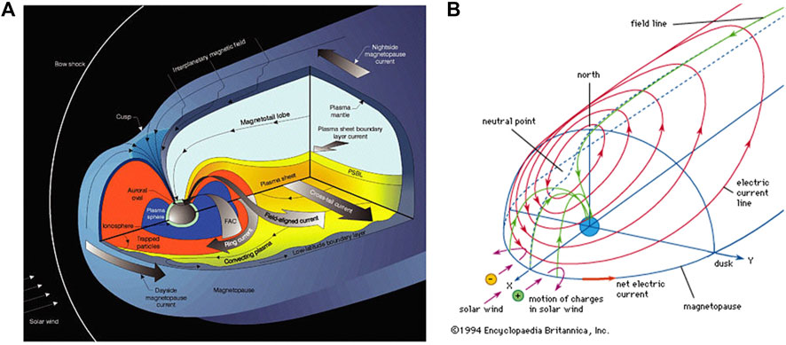
FIGURE 11. (A) Schematic diagram of the Earth’s magnetosphere and current structure with the trapped particles of the inner magnetosphere (representing the radiation belts) shown as the orange region, the plasmasphere shown in blue, while the lobe regions—extending into the magnetotail—are shown in light blue. The currents are represented by the various grey arrows, with the Chapman-Ferraro current (or the magnetopause current) going from dawn to dusk around the magnetopause and the ring current flowing in the opposite dusk to dawn direction further into the inner magnetosphere. The plasma sheet or the magnetotail neutral sheet is then depicted in yellow. Also note the presence of field-aligned currents (FACs) linking the various current systems together to form a coherent system that connects with the Earth’s ionosphere. Image Credit: Pollock et al. (2003). These images were distributed under the https://creativecommons.org/licenses/by/2.0/legalcode Creative Commons Attribution 2.0 International License. (B) Figure of the creation and flow of the Chapman-Ferraro current structure along the dayside magnetopause as positive ions and negative electrons gradient-curvature drift around the magnetopause, creating a net dawn-to-dusk current along the boundary. Note the red curves give the net direction of the Chapman-Ferraro current in its 3D circulation around the magnetopause. Image Credit: Encyclopaedia Britannica.
Moving inward, we then encounter the ring current, located approximately 2–7 Re away from Earth, or roughly between the two radiation belts (Pulkkinen et al., 2017). This current is generated by the gradient curvature drift of keV particles in the inner magnetosphere and flows in the westward direction (Milan et al., 2017) as seen in Figure 10B and Figure 11A. The ring current can be enhanced by ICMEs which tends to drive high ring current activity.
Lastly, the plasmasphere represents a population of cold, low energy (eV) plasma (Li and Hudson, 2019; Lemaire and Gringauz, 1998). The aforementioned magnetospheric electric field defines the boundary of the plasmasphere, called the plasmapause, where dynamic solar wind conditions can either stretch the plasmapause out to the magnetopause, or more tightly confine the plasmasphere (Usanova and Shprits, 2017). This being said, the plasmasphere is normally defined to extend from the Earth’s upper atmosphere (or the ionosphere), out to 4–8 Re (depending on solar wind conditions). Note Figure 11A depicts the plasmasphere as the blue region between the ionosphere and the trapped region (or radiation belts). Magnetospheric convection causes plasma to be drained from the plasmasphere across the plasmapause, while the plasmasphere’s particle population is replenished by ionized particles from Earth’s upper atmosphere (Li and Hudson, 2019).
Now delving into the Earth’s upper atmosphere we encounter the Earth’s ionosphere—layers of ionized gas in the upper atmosphere. Particles in the upper atmosphere become ionized from the Sun’s electromagnetic radiation as well as impacts from magnetospheric energetic electrons (Borovsky and Valdivia, 2018). The ionosphere is particularly important in radio wave propagation around the globe. During the day, the lower layers of the ionosphere (D and E layers) are ionized by sunlight and block access of radio waves to the highest layer, the F layer. But at night, ions in the D and E layers recombine with nearby electrons, so that these layers disappear. The highest layer of the ionosphere, the F layer, has such a low density that recombination does not take place, and the layer remains ionized. Radio waves from the ground are able to then reflect off of the F layer, allowing radio waves to propagate for great distances. As previously mentioned, plasma (cold ions) escapes from the ionosphere through ionospheric outflow and populates the magnetosphere, changing the mass content of near-Earth outer space, including the plasmasphere (Chappell et al., 2008; Kelley, 2009; Schunk and Nagy, 2009; Borovsky and Valdivia, 2018).
4.4 Currents in the Magnetosphere
Currents are created in the magnetosphere through the interaction of the Earth’s magnetic field and the solar wind [see e.g., reviews by Baumjohann et al. (2010), Eastwood et al. (2014), Ganushkina et al. (2015), Ganushkina et al. (2018)]. The structure of the geomagnetic environment is defined by these currents, and responds to a variety of different stimuli. Such stimuli can be a difference in the solar wind pressure (which affects the size of the magnetosphere and their strength). Another stimulus is the orientation and strength of the interplanetary magnetic field (IMF) which modifies the structure of the magnetosphere through magnetic reconnection and allows solar wind plasma to enter into the inner magnetosphere (Milan et al., 2017). Because of this pressure, the dayside is compressed, while the nightside is stretched into the aforementioned magnetotail as can be seen in Figure 11. When the Earth’s magnetic field is distorted into a non-dipolar configuration, where ∇×B ≠ 0, currents are allowed to flow as prescribed by Ampère’s law,
where B is the magnetic field, J is the current density, ɛ0 is the electric constant, and E is the electric field. In most of the space weather applications, the displacement current can be ignored and therefore
For currents in the magnetosphere, the resulting current path is not fixed and can be changed based on the solar wind driving conditions. However, these currents do provide structure to the magnetosphere, like the magnetopause current which provides an essential role in both supporting the structure of the inner magnetosphere and allowing the transport of energy between the solar wind and the inner magnetosphere (Hasegawa, 2012).
The magnetopause current is known as the Chapman-Ferraro current and was first suggested by Chapman and Ferraro (1931). In its simplest form, this current is created by magnetosheath ions and electrons encountering the stronger magnetosphere magnetic field, performing a half-gyration, and then re-entering the magnetosheath as described in Ganushkina et al. (2015) and Baumjohann et al. (2010). This process repeats and eventually creates a net electric current with the particles’ charge controlling the gyration’s direction. Thus, as depicted in Figure 11B, ions gyrate duskward around the magnetopause, while electrons gyrate dawnward (Ganushkina et al., 2018). This leads to a net current running from the dawn to the dusk around the magnetopause while being perpendicular to the magnetic field. The current can also be described by diamagnetic currents, which are generated by ion and electron density and temperature gradients across the magnetopause boundary (Hasegawa, 2012). The current carried by electrons plays an important role in small scale, thin magnetopause current structures (Shuster et al., 2019).
The magnetopause current is essential to our understanding of space weather as this is where magnetic reconnection is believed to take place on the dayside magnetosphere (Trattner et al., 2021). Note this is the same process of magnetic reconnection that reconfigures the solar magnetic field to release magnetic energy in the form of CMEs, flares, and SEPs as described in previous sections. In the case of the magnetopause, magnetic reconnection involves the merging of oppositely directed magnetic field lines, leading to a reconfiguration of the magnetic field and the opening of the magnetosphere’s closed field structure to the influence of the solar wind as reviewed in Hesse and Cassak (2020). This enables the release of energy stored in the magnetic field and creates energetic particles while heating the plasma. As reiterated by Eastwood et al. (2013), reconnection occurs in thin current sheets, like the magnetopause current sheet when the IMF Bz is oriented southward or in the negative Bz direction, which allows energy and plasma from the solar wind to be transferred into the inner magnetosphere by changing the magnetic topology of the Earth’s magnetic field and opening closed field lines as shown in Figure 13 where magnetic reconnection occurs on the dayside magnetopause between the opposing magnetic field lines of the solar wind’s IMF and the Earth’s magnetic field.
The highly stretched magnetospheric tail also has a complex current system. One of the magnetotail currents (the cross-tail current) flows from dawn to dusk flank through the center of the tail; another current makes two loops above and below the central current sheet, closing the cross-tail current through the nighttime magnetopause (Ganushkina et al., 2018). The cross-tail current offsets the differences in magnetic fields and the opposing flow of charges along the magnetotail when it expands (Milan et al., 2017) as depicted in Figure 11A.
These current systems and the different portions of the magnetosphere then “communicate” with one another through field-aligned currents (FACs) as first suggested by Birkeland (1908). So named because they run parallel to the magnetic field, FACs are responsible for circulating plasma between the magnetosphere and ionosphere, creating a complete current system [e.g., Le et al. (2010); Ganushkina et al. (2018)]. This system is allowed to close because of the ionosphere, or the ionized layers of the Earth’s upper atmosphere which provide a conductance, allowing magnetospheric currents to close via the FACs and the Pedersen currents as shown in Figure 12A [e.g., Adhikari et al. (2017)]. The Pedersen currents flow across the polar cap and connect Region 1 and Region 2 field aligned currents. Hall currents follow magnetospheric convection patterns and hence high-latitude ionosphere potential patterns (Milan et al., 2017).
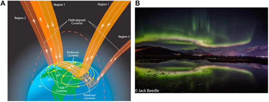
FIGURE 12. (A) Diagram from Le et al. (2010) representing how FACs connect the outer magnetosphere and the ionosphere, where the ionosphere’s conductance allows the current systems to close through the Pedersen currents. (B) Image of the Northern Lights captured over Southeast Alaska, which shows the Northern Lights’ characteristic green curtains (Beedle, 2021).
While FACs all do the same fundamental task, they are further grouped into Region 1 and Region 2 currents as reviewed in Le et al. (2010). Region 1 currents are high latitude currents and connect further out in the magnetosphere to the magnetopause current. Region 2 currents, on the other hand, are lower latitude and connect closer in to the ring current. Altogether, these currents connect the magnetosphere with the ionosphere and help to transfer energy and plasma between the Earth’s magnetosphere and ionosphere in a process known as magnetosphere-ionosphere coupling (Coxon et al., 2015).
4.5 Energy Transfer in the Magnetosphere
4.5.1 The Dungey Cycle
During magnetic reconnection, energy from the solar wind is released in the magnetopause and loaded into the magnetotail where it is stored in the magnetic field until reconnection is triggered in the tail current sheet, allowing the release of energy into the inner magnetosphere as first described by Dungey (1961). This process, as shown in Figure 13, represents the primary way energy is accumulated and released in the outer magnetosphere [e.g., Milan et al. (2007), Milan et al. (2017), Ganushkina et al. (2018)]. In this cycle, the reconnection of the Earth’s magnetic field and the solar wind causes internal circulation and convection of magnetic field and plasma as the solar wind moves past the magnetosphere [e.g., Akasofu (2021)]. When the Bz component of the interplanetary magnetic field (IMF) is negative (solar wind’s magnetic field points in the southward direction), magnetic reconnection can occur at the dayside magnetopause, forming open magnetic field lines that are dragged toward the tail, creating the magnetotail lobes, and storing energy that is then released through magnetic reconnection in the tail (Milan et al., 2007; Lu et al., 2020). This process can be further broken down into the flow of energy, where the solar wind acts as the driver, the magnetopause as the energy intake, the magnetotail as the energy accumulation, and the inner magnetosphere as the net consumer of energy. Additionally, northward IMF solar wind plasma may be directly captured by the inner magnetosphere through magnetic reconnection poleward of the cusp regions (Marcucci et al., 2008). Many magnetospheric phenomena, such as geomagnetic storms and auroral substorms are known to be driven by the solar wind with key aspects of their evolution tied to particular solar wind IMF conditions (Akasofu, 2021).
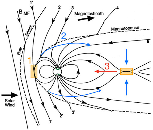
FIGURE 13. Diagram showing the loading of energy from magnetic reconnection in the magnetopause into the magnetotail, which then causes magnetic reconnection in the tail, and unloads the stored energy into the inner magnetosphere. As a cycle this follows the following points: (1) reconnection occurs on the dayside magnetopause, (2) Field lines and plasma convect across the polar cap, loading energy into the magnetotail, and (3) once enough energy is loaded into the tail, reconnection occurs, which sends plasma towards the Earth. Base figure from Eastwood et al. (2017), diagram edited to show main points and colored paths. This image was distributed under the https://creativecommons.org/licenses/by/4.0/legalcode Creative Commons Attribution 2.0 International License.
4.5.2 Substorms
One way the Dungey Cycle transfers energy in the magnetosphere is through substorms, which are the basic loading and unloading process of the magnetosphere [e.g., Valdivia et al. (2005)]. Substorms typically last from 2 to 4 h and represent high latitude magnetic disturbances generated by the solar wind (Partamies et al., 2009), which can be broken into three main phases as reviewed by McPherron and Chu (2016) and Sergeev et al. (2012). The first is called the growth phase where dayside reconnection occurs triggering enhanced convection and the loading of energy at the magnetotail. This leads to the expansion phase, which involves tail reconnection that triggers the unloading of plasma and magnetic flux, and the poleward expansion of the aurora. Lastly, the magnetosphere slowly goes back to pre-storm conditions and the aurora dims in the recovery phase. This substorm process can then be repeated if the solar wind driving conditions continue to cause dayside magnetic reconnection, loading more energy into the magnetotail. How the magnetosphere recovers after a substorm then decides how the substorm is classified. For example, if this process occurs as an isolated event, then it is considered an isolated substorm (Partamies et al., 2009; Sergeev et al., 2012). Recurrent substorms are observed when a significant solar wind perturbation, such as during a geomagnetic storm, triggers a succession of several major and minor substorm cycles that overlap in time, causing random geomagnetic fluctuations, spatially localized tail plasma flows, and a highly dynamic precipitation pattern in the auroral ionosphere (Angelopoulos et al., 1992; Uritsky et al., 2001; Forsyth et al., 2007; Borovsky and Yakymenko, 2017). If the loading and unloading process occurs globally and quasi-periodically, with an approximate period of 2–4 h, then it is called a global sawtooth oscillation (Borovsky, 2004; Partamies et al., 2009). Lastly, if this energy is continually released into the inner magnetosphere instead of being stored in the magnetotail, then it is called a steady magnetospheric convection event [e.g., Partamies et al. (2009)].
During a geomagnetic substorm, compression of the magnetotail causes reconnection on the nightside, leading to depolarization of magnetic field lines and the opposing flow of charged particles along the field lines. This opposing flow of charges induces an E ×B drift of charged particles and plasma towards Earth (Sergeev et al., 2012; McPherron and Chu, 2016), which enhances the inner magnetosphere populations. These charged particles can enter into the ionosphere via field-aligned currents and through a substorm current wedge that is formed during the main phase of the storm (Akasofu, 2021). The substorm current wedge is dynamic and is what allows for plasma to be transferred between Earth’s magnetosphere and ionosphere [e.g., Kepko et al. (2015), McPherron and Chu (2016)]. As reviewed in Akasofu (2021), it is characterized by a drop in the geomagnetic AL index at high latitudes and an increase in AL at low latitudes. The AL index is one of the auroral electrojet indices that measures geomagnetic variations in the horizontal component of Earth’s magnetic field along the northern hemisphere’s auroral oval. Specifically, AL is intended to measure the intensity of the westward auroral electrojet, a current structure that, during substorms, is enhanced by current associated with the substorm current wedge (Ganushkina et al., 2015).
4.5.3 Geomagnetic Storms
On larger scales, geomagnetic storms represent major disturbances of the Earth’s magnetosphere not limited to higher latitudes [e.g., Gonzalez et al. (1994), Haines et al. (2019)]. While substorms represent the basic process for the loading and unloading of energy in the magnetosphere, and thus can be caused under a wide range of solar wind driving conditions, geomagnetic storms (especially strong events) must have a high speed stream or a CME as its driver as it represents a much larger input of energy (Lakhina and Tsurutani, 2016; Vennerstrom et al., 2016). Note that a geomagnetic storm is not necessary to have a substorm, but substorms can occur during geomagnetic storms. However, the exact nature, and existence, of substorm—geomagnetic storm interaction is still a matter of contention and controversy in magnetospheric dynamics (Sharma et al., 2003).
Like substorms, geomagnetic storms can also be broken into different phases which are described by Gonzalez et al. (1994) and Akasofu (2021). The first of these is the sudden storm commencement, which, while not found in all storms, represents a shock impacting the magnetosphere. The growth phase of a geomagnetic storm is often defined by an increase of the geomagnetic disturbance storm time (Dst) index (Klimas et al., 1998). The dayside magnetosphere is compressed, and the flux of the polar cap increases (Vennerstrom et al., 2016). The main phase of a geomagnetic storm is defined by a large and sharp decrease in the Dst index of hundreds of nT. Substorm activity is very active during this time, and the ring current is built up and symmetric [e.g., Lakhina and Tsurutani (2016)]. In addition to the intensification of the global ring current, a significant increase in the energetic particle fluxes in the radiation belts is typically observed during storms. The flux of the polar cap decreases during this period, and the outer layer of the plasmasphere peels off. The recovery phase of a geomagnetic storm is defined by a gradual and steady increase of Dst and the polar cap. The configuration of the magnetosphere will gradually revert back to pre-initial phase conditions. The plasmasphere will have a plume due to the disruption and geomagnetic storm activity, which may reach past the magnetopause (Akasofu, 2021).
4.5.4 Viscous Interaction
While the open magnetosphere and the Dungey cycle represent the majority of energy transfer into the Earth’s magnetosphere (Dungey, 1961), these conditions require an IMF negative (southward) Bz for the solar wind to impart its energy to the magnetosphere through magnetic reconnection on the dayside magnetopause. If the IMF Bz is positive (northward), energy is still transferred into the magnetosphere, albeit at a much slower rate [e.g., Tsurutani and Gonzalez (1995), Borovsky (2013)]. This process is called viscous interaction as first defined by Axford and Hines (1961) and represents the fact that the magnetopause current sheet is still created even in these positive, (northward) Bz conditions. As discussed by Masters (2018) for a planet with a magnetic field, solar wind ions impact the magnetopause and gyrate across it creating a current. This leads to the build up of negative and positive charge on the flanks of the magnetopause into the magnetotail. These opposite charges then create an electric field which causes plasma in the magnetotail to bulk drift toward the inner magnetosphere. While this mechanism is present in both the open and closed magnetosphere, unlike the Dungey Cycle, it contributes much less to the energy transfer in the magnetosphere overall as previously discussed.
5 Space Weather as an Interconnected System
The entire space weather system may be viewed as a complex interconnection between the Sun and the Earth, as shown in Figure 14. In particular, it describes phenomena that impact systems and technologies in orbit and on the Earth [e.g., Piersanti et al. (2017), Piersanti et al. (2020)]. As the previous sections have shown, the internal structure of the Sun has an inner layer of plasma that differentially rotates creating the solar dynamo and generating the Sun’s magnetic field. Some solar structures, such as coronal holes, have “open” magnetic field lines and generate high speed solar wind streams, which extend beyond the Sun creating space weather conditions in interplanetary space and at Earth. This differential rotation also influences the solar cycle as it can distort the magnetic field and is one of the factors that builds up magnetic energy in the form of flux ropes, as the cycle starts from a solar quiet system and progresses into an increasingly disoriented solar maximum system, in which the solar magnetic field is complex. During high solar activity, the magnetic poles of the Sun are reversed.
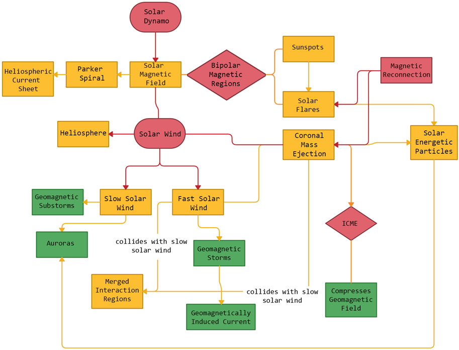
FIGURE 14. Flow chart depicting the interconnected nature of the space weather system with connections between various space weather phenomena and structures in the solar system covered by this review paper.
Magnetic reconnection then contributes kinetic and thermal energy to the solar plasma, further aiding the development of instabilities. Such instabilities in magnetic flux tubes triggers magnetic reconnection as the fundamental driver for space weather events, as illustrated in Figure 14.
The “open” field lines coupled with the Sun’s rotation form a solar spiral, whose orientation influences the space weather system outside of the solar atmosphere and into the heliosphere. For example, the propagation of charged particles such as SEPs tend to follow the field lines of the Parker spiral because of electromagnetic interactions which cause these charged particles to gyrate along the axis of the magnetic field lines as they propagate away from the Sun as discussed in Section 3.2. Particles accelerated at the Sun leading to SEP events can penetrate Earth’s magnetosphere and reach the upper atmosphere where they can create hazards to both human health and electronic components (García-Rigo et al., 2016). Gradual SEP events, which often occur in swarms, tend to pose a larger risk than impulsive ones (Klein and Dalla, 2017).
In addition, the ambient solar wind influences the outward propagation of interplanetary shocks and ICMEs, where interplanetary shocks may accelerate particles in their path of propagation [e.g., Pallocchia et al. (2017)]. High-speed streams can create regions of compressed and turbulent plasma when it interacts with the slower-moving ambient solar wind.
This highly structured solar plasma outflow influences the magnetosphere through the Dungey cycle causing the storage of energy in the magnetotail and resulting in magnetic reconnection on the night-side allowing the interaction between the charged particles carried by solar wind with Earth’s upper atmosphere.
Because these electrons and protons are very energetic, when they collide with atoms and molecules of oxygen, nitrogen, etc. in Earth’s upper atmosphere, they excite these particles, which causes them to radiate (Schroeder et al., 2021). This process is described in Russell et al. (2016) and an example of the results can be seen in Figure 12B, where the aurora is composed of many different colors, which correspond to what type of atom or molecule was excited. For example, oxygen typically creates the green glow that comprises the bulk of aurora, while atomic nitrogen can cause a blue glow (Lummerzheim, 2009). As aurora are driven by these charged particles, large displays of aurora require large influxes of plasma into the upper atmosphere like during the Dungey cycle with substorms and geomagnetic storms. Additionally, the closer the aurora is seen to the equator, the stronger the solar wind driving conditions must be, such as during fast moving CME events.
While the aurora is a magnificent display of the vast quantities of energy the Sun imparts to Earth’s magnetosphere, other types of energy transfer can also have detrimental effects on our modernizing infrastructure. For example, a solar flare can produce strong X-rays that degrade (or often block) high-frequency radio waves used in radio communications (Frissell et al., 2019). They reach Earth in a matter of 8 min and are called radio blackouts storms. Additionally, during perturbed geomagnetic conditions, such as after the impact of an ICME, other magnetospheric currents such as field-aligned (or Birkeland) currents will transfer energy and plasma between the Earth’s magnetosphere and ionosphere in the process of magnetosphere-ionosphere coupling (Coxon et al., 2015). This directly has an impact on satellites in high latitudes such as satellites at geosynchronous orbits. Such events can also cause effects like radio blackouts that can disrupt electronics both in orbit and on Earth.
These events can also result in substantial geomagnetically induced currents (GICs) through electromagnetic induction as depicted in Pulkkinen et al. (2017). The GICs can have major effects on the ground, such as increasing corrosion in buried oil and gas pipelines and saturating transformers of power grids causing black-outs or permanent damage (Pulkkinen, 2007). As discussed above, CMEs can create a handful of effects, such as the auroras, GICs, and geomagnetic storms that can modify the signal from radio navigation systems (GPS and GNSS) causing degraded accuracy. Additionally, influxes of radiation and charged particles, such as during SEP events that produce ground level enhancements, can harm satellites and prove potentially hazardous for manned space missions.
To summarize, what happens on the Sun directly and indirectly affects the conditions in the heliosphere which directly affects the conditions of Earth’s magnetosphere, which in turn can affect our daily lives. The entire system is vastly interconnected, and each part of the system has a significant role to play in the cosmic dance of the heliosphere and its dynamics. The diagram in Figure 15 shows a plethora of potential impacts that space weather can have on society, highlighting the importance of research in the overall field.
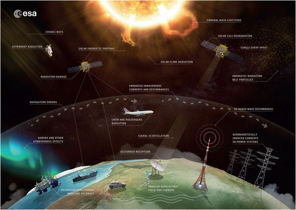
FIGURE 15. Illustration of the many societal effects that space weather can cause. Effects include damage to electronic in orbit around Earth, radiation risks to astronauts and airline passengers, telecommunication disturbances such as radio and GPS blackouts, and risks to power grid disruptions Cranmer et al. (2017). Image Credits: European Space Agency (ESA).
The increasing importance of space weather to our advancing society has given rise to the field of space weather predictions, where complex models are used to predict space weather events and their propagation throughout the heliosphere. One important tool to the space weather modeling community is the Community Coordinated Modeling Center, or CCMC, at NASA Goddard Space Flight Center, which provides simulation runs on various space weather models and scores their accuracy (Eastwood et al., 2017). While the scope of this paper limits us from discussing space weather forecasting further, Eastwood et al. (2017) provides a comprehensive review on the foundations of magnetospheric space weather forecasting, and Cicogna et al. (2021) and Stumpo et al. (2021) provide useful discussion on the forecasting of solar flares and SEP events, respectively.
6 Conclusion
This “user’s guide” or first-step paper was designed towards understanding the magnetically connected space weather system for those unfamiliar with the main topics of the field. Because space weather is a vast discipline covering a plethora of interconnected systems, it is difficult to review the basic concepts of the system in a way that is understandable and brief. Thus, this paper aims to explore the basics of the space weather system and how it affects our daily lives for those who may not necessarily have the time, resources, or expertise to comb through the vast scientific literature necessary to understand this topic. The authors believe a general understanding of space weather is important for an increasing number of people and professions as technology, often susceptible to space weather events, continues to play an ever larger role in our daily lives.
As a system, the magnetic interconnectivity of space weather can be summarized in the following ways:
1. Subsurface flows of plasma in the solar interior store and gradually build up energy as they drag solar magnetic field lines along with the flows of plasma, causing kinks in the Sun’s magnetic field and leading to the storage of energy in magnetic flux ropes. This buildup of energy is then released through magnetic reconnection, resulting in the rapid eruption of solar material and magnetic field in the form of space weather phenomena such as CMEs, solar flares, and SEP events.
2. Magnetic reconnection frees energy from the magnetic field to transfer to the solar wind. The properties of the solar wind and space weather events such as CMEs etc. are a direct consequence of magnetic reconnection on the Sun. The solar wind transports the magnetic configuration of the Sun to the interplanetary medium.
3. After traveling through the heliosphere, the solar wind impacts Earth’s magnetic field, imparting its energy through magnetic reconnection on the magnetopause. This energy is then diverted into Earth’s upper atmosphere through magnetic reconnection on the magnetotail during geomagnetic storms and substorms, allowing for the creation of the iconic aurora and the energization of the Earth’s local environment.
Based on these processes, the different space weather events driven by magnetic reconnection have an impact on our daily lives. These impacts can be seen from outer space, such as effects on astronauts and satellites, to effects on power grids and pipelines on the ground. Due to the society’s dependence on technology, the importance of the understanding of these processes are crucial to better prepare for these events.
Author Contributions
JB—wrote magnetosphere section, main editor, worked on conclusion. CR—wrote solar section, general editing/structure, worked on conclusion, managed figures. DS—general editing/structure, magnetosphere section literature review. HC—wrote heliosphere section. VM—wrote interconnectivity section, general editing/structure, compiled bibliography, worked on conclusion, solar section literature review. VU—wrote introduction/abstract, funding, general structure, introduction literature review, general literature review.
Funding
This work was partly supported through cooperative agreements NNG11PL10A and 80NSSC21M0180 between NASA Goddard Space Flight Center and the Catholic University of America.
Conflict of Interest
The authors declare that the research was conducted in the absence of any commercial or financial relationships that could be construed as a potential conflict of interest.
Publisher’s Note
All claims expressed in this article are solely those of the authors and do not necessarily represent those of their affiliated organizations, or those of the publisher, the editors and the reviewers. Any product that may be evaluated in this article, or claim that may be made by its manufacturer, is not guaranteed or endorsed by the publisher.
Acknowledgments
The authors thank E. D. Fletcher, M. Jeunon, J. R. Mejia-Ott, J. Nosowitz, and L. M. Vazhayil Kurien for their assistance with the initial evaluation of the reviewed material and useful discussions. The authors also thank Dr. Anna DeJong for insightful discussions regarding space weather systems. Additionally, the authors thank Jack Beedle for the use of his Northern Lights photography.
Footnotes
1SI units are used in equations throughout this paper.
References
Adhikari, B., Dahal, S., and Chapagain, N. P. N. (2017). Study of Field-Aligned Current (FAC), Interplanetary Electric Field Component (E Y ), Interplanetary Magnetic Field Component (B Z ), and Northward (X ) and Eastward (Y ) Components of Geomagnetic Field during Supersubstorm. Earth Space Sci. 4, 257–274. doi:10.1002/2017EA000258
Akasofu, S.-I. (2021). A Review of Studies of Geomagnetic Storms and Auroral/magnetospheric Substorms Based on the Electric Current Approach. Front. Astron. Space Sci. 7. doi:10.3389/fspas.2020.604750
Anderson, B. (2004). Course Notes for Space Physics. Baltimore, MD: Johns Hopkins University, 615755. (Unpublished).
Angelopoulos, V., Baumjohann, W., Kennel, C. F., Coroniti, F. V., Kivelson, M. G., Pellat, R., et al. (1992). Bursty Bulk Flows in the Inner Central Plasma Sheet. J. Geophys. Res. 97, 4027–4039. doi:10.1029/91JA02701
Antiochos, S. K., DeVore, C. R., and Klimchuk, J. A. (1999). A Model for Solar Coronal Mass Ejections. ApJ 510, 485–493. doi:10.1086/306563
Antiochos, S. K. (1998). The Magnetic Topology of Solar Eruptions. Astrophysical J. Lett. 502, L181–L184. doi:10.1086/311507
Axford, W. I., and Hines, C. O. (1961). A Unifying Theory of High-Latitude Geophysical Phenomena and Geomagnetic Storms. Can. J. Phys. 39, 1433–1464. doi:10.1029/GM018p0936
Bai, T., and Sturrock, P. A. (1989). Classification of Solar Flares. Annu. Rev. Astron. Astrophys. 27, 421–467. doi:10.1146/annurev.aa.27.090189.002225
Baumjohann, W., Blanc, M., Fedorov, A., and Glassmeier, K.-H. (2010). Current Systems in Planetary Magnetospheres and Ionospheres. Space Sci. Rev. 152, 99–134. doi:10.1007/s11214-010-9629-z
Bazilevskaya, G. A., Cliver, E. W., Kovaltsov, G. A., Ling, A. G., Shea, M. A., Smart, D. F., et al. (2015). Solar Cycle in the Heliosphere and Cosmic Rays. Space Sci. Ser. ISSI Solar Activity Cycle 2015, 409–435. doi:10.1007/978-1-4939-2584-1_14
Birkeland, K. (1908). The Norwegian Aurora Polaris Expedition, 1902-1903. On the Cause of Magnetic Storms and the Origin of Terrestrial Magnetism. Oslo, Norway: Aschehoug and Co.
Borovsky, J. E. (2013). Physics-based Solar Wind Driver Functions for the Magnetosphere: Combining the Reconnection-Coupled Mhd Generator with the Viscous Interaction. J. Geophys. Res. Space Phys. 118, 7119–7150. doi:10.1002/jgra.50557
Borovsky, J. E., and Valdivia, J. A. (2018). The Earth's Magnetosphere: A Systems Science Overview and Assessment. Surv. Geophys. 39, 817–859. doi:10.1007/s10712-018-9487-x
Borovsky, J. E., and Yakymenko, K. (2017). Substorm Occurrence Rates, Substorm Recurrence Times, and Solar Wind Structure. J. Geophys. Res. Space Phys. 122, 2973–2998. doi:10.1002/2016JA023625
Borovsky, J. (2004). Global Sawtooth Oscillations of the Magnetosphere. Eos Trans. AGU 85, 525. doi:10.1029/2004eo490009
Borrero, J. M., and Ichimoto, K. (2011). Magnetic Structure of Sunspots. Living Rev. Sol. Phys. 8, 4. doi:10.12942/lrsp-2011-4
Bruno, R. (2019). Intermittency in Solar Wind Turbulence from Fluid to Kinetic Scales. Earth Space Sci. 6, 656–672. doi:10.1029/2018EA000535
Burlaga, L. F., Ness, N. F., Acuña, M. H., Lepping, R. P., Connerney, J. E. P., Stone, E. C., et al. (2005). Crossing the Termination Shock into the Heliosheath: Magnetic fields. Science 309, 2027–2029. doi:10.1126/science.1117542
Cameron, R. H., Dikpati, M., and Brandenburg, A. (2017). The Global Solar Dynamo. Space Sci. Rev. 210, 367–395. doi:10.1007/s11214-015-0230-3
Chapman, S., and Ferraro, V. C. A. (1931). A New Theory of Magnetic Storms. J. Geophys. Res. 36, 77–97. doi:10.1029/TE036i002p00077
Chappell, C. R., Huddleston, M. M., Moore, T. E., Giles, B. L., and Delcourt, D. C. (2008). Observations of the Warm Plasma Cloak and an Explanation of its Formation in the Magnetosphere. J. Geophys. Res. 113, a–n. doi:10.1029/2007JA012945
Charbonneau, P. (2010). Dynamo Models of the Solar Cycle. Living Rev. Solar Phys. 7. doi:10.12942/lrsp-2010-3
Christensen-Dalsgaard, J., Gough, D. O., and Thompson, M. J. (1991). The Depth of the Solar Convection Zone. ApJ 378, 413. doi:10.1086/170441
Cicogna, D., Berrilli, F., Calchetti, D., Del Moro, D., Giovannelli, L., Benvenuto, F., et al. (2021). Flare-forecasting Algorithms Based on High-Gradient Polarity Inversion Lines in Active Regions. ApJ 915, 38. doi:10.3847/1538-4357/abfafb
Cliver, E. W., Dennis, B. R., Kiplinger, A. L., Kane, S. R., Neidig, D. F., Sheeley, N. R. J., et al. (1986). Solar Gradual Hard X-Ray Bursts and Associated Phenomena. Astrophysical J. 305, 920. doi:10.1086/164306
Cliver, E. W. (2016). Flare versus Shock Acceleration of High-Energy Protons in Solar Energetic Particle Events. ApJ 832, 128. doi:10.3847/0004-637x/832/2/128
Coxon, J. C., Milan, S. E., Clausen, L. B. N., Anderson, B. J., and Korth, H. (2015). The Magnitudes of the Regions 1 and 2 Birkeland Currents Observed by Ampere and Their Role in Solar Wind-Magnetosphere-Ionosphere Coupling. J. Geophys. Res. Space Phys. 119, 9804–9815. doi:10.1002/2014JA020138
Cranmer, S. R., Gibson, S. E., and Riley, P. (2017). Origins of the Ambient Solar Wind: Implications for Space Weather. Space Sci. Rev. 212, 1345–1384. doi:10.1007/s11214-017-0416-y
Desai, M., and Giacalone, J. (2016). Large Gradual Solar Energetic Particle Events. Living Rev. Sol. Phys. 13. doi:10.1007/s41116-016-0002-5
Discola Junior, S. L. (2019). Enhancing Solar Flare Forecasting: a Multi-Class and Mulit-Label Classification Approach to Handel Imbalanced Time Series. Ph.D. thesis. São Carlos: Federal University of São Carlos.
Dungey, J. W. (1961). Interplanetary Magnetic Field and the Auroral Zones. Phys. Rev. Lett. 6, 47–48. doi:10.1103/physrevlett.6.47
Dungey, J. W. (1953). Lxxvi. Conditions for the Occurrence of Electrical Discharges in Astrophysical Systems. Lond. Edinb. Dublin Philosophical Mag. J. Sci. 44, 725–738. doi:10.1080/14786440708521050
Eastwood, J. P., Hietala, H., Toth, G., Phan, T. D., and Fujimoto, M. (2014). What Controls the Structure and Dynamics of Earth’s Magnetosphere? Space Sci. Rev. 188, 251–286. doi:10.1007/s11214-014-0050-x
Eastwood, J. P., Nakamura, R., Turc, L., Mejnertsen, L., and Hesse, M. (2017). The Scientific Foundations of Forecasting Magnetospheric Space Weather. Space Sci. Rev. 212, 1221–1252. doi:10.1007/s11214-017-0399-8
Eastwood, J. P., Phan, T. D., Øieroset, M., Shay, M. A., Malakit, K., Swisdak, M., et al. (2013). Influence of Asymmetries and Guide fields on the Magnetic Reconnection Diffusion Region in Collisionless Space Plasmas. Plasma Phys. Controlled Fusion 55, 124001. doi:10.1088/0741-3335/55/12/124001
Fahr, H.-J. (2004). Global Structure of the Heliosphere and Interaction with the Local Interstellar Medium: Three Decades of Growing Knowledge. Adv. Space Res. 34, 3–13. doi:10.1016/j.asr.2003.02.052
Forbes, T. G. (2000). A Review on the Genesis of Coronal Mass Ejections. J. Geophys. Res. Space Phys. 105, 23153–23165. doi:10.1029/2000JA000005
Forsyth, C., Lester, M., Cowley, S. W., Dandouras, I., Fazakerley, A. N., Fear, R. C., et al. (2007). “Observed Tail Current Systems Associated with Bursty Bulk Flows and Auroral Streamers during a Period of Multiple Substorms,” in AGU Fall Meeting Abstracts, 2007, SM23A–1178.
Frissell, N. A., Vega, J. S., Markowitz, E., Gerrard, A. J., Engelke, W. D., Erickson, P. J., et al. (2019). High-frequency Communications Response to Solar Activity in September 2017 as Observed by Amateur Radio Networks. Space Weather 17, 118–132. doi:10.1029/2018SW002008
Ganushkina, N. Y., Liemohn, M. W., and Dubyagin, S. (2018). Current Systems in the Earths Magnetosphere. Rev. Geophys. 56, 309–332. doi:10.1002/2017rg000590
Ganushkina, N. Y., Liemohn, M. W., Dubyagin, S., Daglis, I. A., Dandouras, I., Zeeuw, D. L. D., et al. (2015). Defining and Resolving Current Systems in Geospace. Ann. Geophysicae 33, 1369–1402. doi:10.5194/angeo-33-1369-2015
García-Rigo, A., Núñez, M., Qahwaji, R., Ashamari, O., Jiggens, P., Pérez, G., et al. (2016). Prediction and Warning System of Sep Events and Solar Flares for Risk Estimation in Space Launch Operations. J. Space Weather Space Clim. 6. doi:10.1051/swsc/2016021
Georgoulis, M. K., Nindos, A., and Zhang, H. (2019). The Source and Engine of Coronal Mass Ejections. Philosophical Trans. R. Soc. A: Math. Phys. Eng. Sci. 377, 20180094. doi:10.1098/rsta.2018.0094
Giovanelli, R. G. (1947). Magnetic and Electric Phenomena in the Sun’s Atmosphere Associated with Sunspots. Monthly Notices R. Astronomical Soc. 107, 338. doi:10.1093/mnras/107.4.338
Glatzmaier, G. A., and Roberts, P. H. (1995). A Three-Dimensional Convective Dynamo Solution with Rotating and Finitely Conducting Inner Core and Mantle. Phys. Earth Planet. Interiors 91, 63–75. doi:10.1016/0031-9201(95)03049-3
Gombosi, T. I., Holst, B. V. D., Manchester, W. B., and Sokolov, I. V. (2018). Extended Mhd Modeling of the Steady Solar corona and the Solar Wind. Living Rev. Solar Phys. 15. doi:10.1007/s41116-018-0014-4
Gonzalez, W. D., Joselyn, J. A., Kamide, Y., Kroehl, H. W., Rostoker, G., Tsurutani, B. T., et al. (1994). What Is a Geomagnetic Storm? J. Geophys. Res. Space Phys. 99, 5771–5792. doi:10.1029/93JA02867
Gosling, J. T. (1993). The Solar Flare Myth. J. Geophys. Res. Space Phys. 98, 18937–18949. doi:10.1029/93ja01896
Gray, D. F. (2005). “Background,” in The Observation and Analysis of Stellar Photospheres. 3 edn. (Cambridge University Press), 1–25. doi:10.1017/CBO9781316036570.004
Green, L. M., Török, T., Vršnak, B., Manchester, W., and Veronig, A. (2018). The Origin, Early Evolution and Predictability of Solar Eruptions. Space Sci. Rev. 214. doi:10.1007/s11214-017-0462-5
Gubbins, D. (1974). Theories of the Geomagnetic and Solar Dynamos. Rev. Geophys. 12, 137–154. doi:10.1029/rg012i002p00137
Guo, F., Giacalone, J., and Zhao, L. (2021). Shock Propagation and Associated Particle Acceleration in the Presence of Ambient Solar-Wind Turbulence. Front. Astron. Space Sci. 8, 27. doi:10.3389/fspas.2021.644354
Gurnett, D. A., Kurth, W. S., Burlaga, L. F., and Ness, N. F. (2013). In Situ observations of Interstellar Plasma with Voyager 1. Science 341, 1489–1492. doi:10.1126/science.1241681
Habbal, S. R., Woo, R., Fineschi, S., Oneal, R., Kohl, J., Noci, G., et al. (1997). Origins of the Slow and the Ubiquitous Fast Solar Wind. Astrophysical J. 489. doi:10.1086/310970
Haines, C., Owens, M. J., Barnard, L., Lockwood, M., and Ruffenach, A. (2019). The Variation of Geomagnetic Storm Duration with Intensity. Solar Phys. 294. doi:10.1007/s11207-019-1546-z
Hasegawa, H. (2012). Structure and Dynamics of the Magnetopause and its Boundary Layers. Monogr. Environ. Earth Planets 1, 71–119. doi:10.5047/meep.2012.00102.0071
Hathaway, D. H. (1994). Producing the Solar Dynamo. Eos, Trans. Am. Geophys. Union 75, 548. doi:10.1029/94eo02032
Hesse, M., and Cassak, P. A. (2020). Magnetic Reconnection in the Space Sciences: Past, Present, and Future. J. Geophys. Res. Space Phys. 125. doi:10.1029/2018JA025935
Hu, J., Li, G., Ao, X., Zank, G., and Verkhoglyadova, O. (2017). Modeling Particle Acceleration and Transport at a 2-d Cme-Driven Shock. J. Geophys. Res. Space Phys. 122. doi:10.1002/2017ja024077
Janvier, M., Aulanier, G., and Démoulin, P. (2015). From Coronal Observations to Mhd Simulations, the Building Blocks for 3d Models of Solar Flares (Invited Review). Solar Phys. 290, 3425–3456. doi:10.1007/s11207-015-0710-3
Jeffrey, N., Kontar, E., and Fletcher, L. (2019). The Role of Energy Diffusion in the Deposition of Energetic Electron Energy in Solar and Stellar Flares. Astrophysical J. 880, 136. doi:10.3847/1538-4357/ab2764
Kahler, S. W. (2003). Probing the Magnetic Polarity Structure of the Heliospheric Current Sheet. J. Geophys. Res. 108. doi:10.1029/2002ja009649
Kanani, S., Arridge, C., Jones, G. J., Fazakerley, A., McAndrews, H., Sergis, N., et al. (2010). A New Form of Saturn’s Magnetopause Using a Dynamic Pressure Balance Model, Based on In Situ, Multi-Instrument Cassini Measurements. J. Geophys. Res. 115. doi:10.1029/2009JA014262
Kelley, M. (2009). The Earth’s Ionosphere: Plasma Physics and Electrodynamics. 2nd ed. Academic Press.
Kepko, L., McPherron, R. L., Amm, O., Apatenkov, S., Baumjohann, W., Birn, J., et al. (2015). Substorm Current Wedge Revisited. Space Sci. Rev. 190, 1–46. doi:10.1007/s11214-014-0124-9
Kilpua, E., Koskinen, H. E. J., and Pulkkinen, T. I. (2017). Coronal Mass Ejections and Their Sheath Regions in Interplanetary Space. Living Rev. Solar Phys. 14. doi:10.1007/s41116-017-0009-6
Klein, K.-L., and Dalla, S. (2017). Acceleration and Propagation of Solar Energetic Particles. Space Sci. Rev. 212, 1107–1136. doi:10.1007/s11214-017-0382-4
Klimas, A. J., Vassiliadis, D., and Baker, D. N. (1998). Dst index Prediction Using Data-Derived Analogues of the Magnetospheric Dynamics. J. Geophys. Res. – Space Phys. 103, 20435–20448. doi:10.1029/98JA01559
Knipp, D. J., and Gannon, J. L. (2019). The 2019 National Space Weather Strategy and Action Plan and beyond. Space Weather 17, 794–795. doi:10.1029/2019SW002254
Kulsrud, R. M. (1998). Magnetic Reconnection in a Magnetohydrodynamic Plasma. Phys. Plasmas 5, 1599–1606. doi:10.1063/1.872827
Laitinen, T., and Dalla, S. (2019). From Sun to Interplanetary Space: What Is the Pathlength of Solar Energetic Particles? Astrophysical J. 887, 222. doi:10.3847/1538-4357/ab54c7
Lakhina, G. S., and Tsurutani, B. T. (2016). Geomagnetic Storms: Historical Perspective to Modern View. Geosci. Lett. 3. doi:10.1186/s40562-016-0037-4
Le, G., Slavin, J. A., and Strangeway, R. J. (2010). Space Technology 5 Observations of the Imbalance of Regions 1 and 2 Field-Aligned Currents and its Implication to the Cross-Polar Cap Pedersen Currents. J. Geophys. Res. Space Phys. 115, A07202. doi:10.1029/2009ja014979
Leake, J. E., and Arber, T. D. (2006). The Emergence of Magnetic Flux through a Partially Ionised Solar Atmosphere. Astron. Astrophysics 450, 805–818. doi:10.1051/0004-6361:20054099
Leake, J. E., Linton, M. G., and Török, T. (2013). Simulations of Emerging Magnetic Flux. I. The Formation of Stable Coronal Flux Ropes. Astrophysical J. 778, 99. doi:10.1088/0004-637x/778/2/99
Li, W., and Hudson, M. (2019). Earths Van allen Radiation Belts: From Discovery to the Van allen Probes Era. J. Geophys. Res. Space Phys. 124, 8319–8351. doi:10.1029/2018ja025940
Liu, R. (2020). Magnetic Flux Ropes in the Solar corona: Structure and Evolution toward Eruption. Res. Astron. Astrophysics 20, 165. doi:10.1088/1674-4527/20/10/165
Lu, S., Wang, R., Angelopoulos, V., Nakamura, R., Artemyev, A. V., Pritchett, T. Z., et al. (2020). Magnetotail Reconnection Onset Caused by Electron Kinetics with a strong External Driver. Nat. Commun. 11. doi:10.1038/s41467-020-18787-w
Mandea, M., and Chambodut, A. (2020). Geomagnetic Field Processes and Their Implications for Space Weather. Surv. Geophys. 41, 1611–1627. doi:10.1007/s10712-020-09598-1
Marcucci, M. F., Coco, I., Ambrosino, D., Amata, E., Milan, S. E., Bavassano Cattaneo, M. B., et al. (2008). Extended Superdarn and Image Observations for Northward Imf: Evidence for Dual Lobe Reconnection. J. Geophys. Res. 113. doi:10.1029/2007JA012466
Masters, A. (2018). A More Viscous-like Solar Wind Interaction with All the Giant Planets. Geophys. Res. Lett. 45, 7320–7329. doi:10.1029/2018GL078416
Matsumoto, R., and Shibata, K. (1992). Three-Dimensional MHD Simulation of the Parker Instability in Galactic Gas Disks and the Solar Atmosphere. Astronom. Soc. Jpn. 44, 167–175.
Mauk, B. H., Fox, N. J., Kanekal, S. G., Kessel, R. L., Sibeck, D. G., and Ukhorskiy, A. (2013). Science Objectives and Rationale for the Radiation belt Storm Probes mission. Space Sci. Rev. 179, 3–27. doi:10.1007/s11214-012-9908-y
McPherron, R. L., and Chu, X. (2016). Relation of the Auroral Substorm to the Substorm Current Wedge. Geosci. Lett. 3. doi:10.1186/s40562-016-0044-5
Mierla, M., Davila, J., Thompson, W., Inhester, B., Srivastava, N., Kramar, M., et al. (2008). A Quick Method for Estimating the Propagation Direction of Coronal Mass Ejections Using Stereo-Cor1 Images. Solar Phys. 252, 385–396. doi:10.1007/s11207-008-9267-8
Milan, S. E., Clausen, L. B. N., Coxon, J. C., Carter, J. A., Walach, M.-T., Laundal, K., et al. (2017). Overview of Solar Wind–Magnetosphere–Ionosphere–Atmosphere Coupling and the Generation of Magnetospheric Currents. Space Sci. Rev. 206, 547–573. doi:10.1007/s11214-017-0333-0
Milan, S. E., Provan, G., and Hubert, B. (2007). Magnetic Flux Transport in the Dungey Cycle: A Survey of Dayside and Nightside Reconnection Rates. J. Geophys. Res. 112. doi:10.1029/2006JA011642
Mishev, A., and Usoskin, I. (2020). Current Status and Possible Extension of the Global Neutron Monitor Network. J. Space Weather Space Clim. 10, 17. doi:10.1051/swsc/2020020
Pallavicini, R., Serio, S., and Vaiana, G. S. (1977). A Survey of Soft X-ray Limb Flare Images: the Relation between Their Structure in the corona and Other Physical Parameters. Astrophysical J. 216, 108–122. doi:10.1086/155452
Pallocchia, G., Laurenza, M., and Consolini, G. (2017). On Weibull’s Spectrum of Nonrelativistic Energetic Particles at. IP shocks: Observations Theor. interpretation 837, 158. doi:10.3847/1538-4357/aa633a
Parker, E. N. (1963). The Solar-Flare Phenomenon and the Theory of Reconnection and Annihiliation of Magnetic fields. Astrophysical J. Suppl. Ser. 8, 177. doi:10.1086/190087
Partamies, N., Pulkkinen, T. I., McPherron, R. L., McWilliams, K., Bryant, C. R., Tanskanen, E., et al. (2009). Statistical Survey on Sawtooth Events, Smcs and Isolated Substorms. Adv. Space Res. 44, 376–384. doi:10.1016/j.asr.2009.03.013
Piersanti, M., De Michelis, P., Del Moro, D., Tozzi, R., Pezzopano, M., Consolini, G., et al. (2017). Comprehensive Analysis of the Geoeffective Solar Event of 21 June 2015: Effects on the Magnetosphere, Plasmasphere, and Ionosphere Systems. Sol. Phys. 292. doi:10.1007/s11207-017-1186-0
Piersanti, M., De Michelis, P., Del Moro, D., Tozzi, R., Pezzopane, M., Consolini, G., et al. (2020). From the Sun to Earth: Effects of the 25 August 2018 Geomagnetic Storm. Ann. Geophysicae 38, 703–724. doi:10.5194/angeo-38-703-2020
Pizzo, V. (1978). A Three-Dimensional Model of Corotating Streams in the Solar Wind, 1. Theoretical Foundations. J. Geophys. Res. 83, 5563. doi:10.1029/ja083ia12p05563
Plainaki, C., Mavromichalaki, H., Laurenza, M., Gerontidou, M., Kanellakopoulos, A., and Storini, M. (2014). The Ground-Level Enhancement of 2012 May 17: Derivation of Solar Proton Event Properties through the Application of the Nmbangle Ppola Model. Astrophysical J. 785, 160. doi:10.1088/0004-637x/785/2/160
Pollock, C. J., C:son-Brandt, P., Burch, J. L., Henderson, M. G., Jahn, J.-M., Mccomas, D. J., et al. (2003). The Role and Contributions of Energetic Neutral Atom (Ena) Imaging in Magnetospheric Substorm Research. Magnetospheric Imaging — The Image Prime Mission 109, 155–182. doi:10.1007/978-94-010-0027-7_8
Pulkkinen, A., Bernabeu, E., Thomson, A., Viljanen, A., Pirjola, R., Boteler, D., et al. (2017). Geomagnetically Induced Currents: Science, Engineering, and Applications Readiness. Space Weather 15, 828–856. doi:10.1002/2016SW001501
Pulkkinen, T. (2007). Space Weather: Terrestrial Perspective. Living Rev. Solar Phys. 4. doi:10.12942/lrsp-2007-1
Reames, D. V. (1999). Particle Acceleration at the Sun and in the Heliosphere. Space Sci. Rev. 90. doi:10.1023/a:1005105831781
Richardson, I. G. (2018). Solar Wind Stream Interaction Regions throughout the Heliosphere. Living Rev. Solar Phys. 15. doi:10.1007/s41116-017-0011-z
Riley, P., Linker, J. A., Mikić, Z., Lionello, R., Ledvina, S. A., and Luhmann, J. G. (2006). A Comparison between Global Solar Magnetohydrodynamic and Potential Field Source Surface Model Results. Astrophysical J. 653, 1510–1516. doi:10.1086/508565
Roberts, P. H. (2007). Alfvéns Theorem and the Frozen Flux Approximation. Encyclopedia of Geomagnetism and Paleomagnetism 7, 07–11. doi:10.1007/978-1-4020-4423-6_5
Russell, C. T., Luhmann, J. G., and Strangeway, R. J. (2016). Space Physics. reprint edn. illustrated: Cambridge University Press.
Scherrer, P. H., Schou, J., Bush, R. I., Kosovichev, A. G., Bogart, R. S., Hoeksema, J. T., et al. (2011). The Helioseismic and Magnetic Imager (Hmi) Investigation for the Solar Dynamics Observatory (Sdo). The Solar Dyn. Observatory, 207–227. doi:10.1007/978-1-4614-3673-7_10
Schmitt, D. (1987). An alpha-omega-dynamo with an Alpha-Effect Due to Magnetostrophic Waves. Astron. Astrophysics 174, 281–287.
Schroeder, J. W. R., Howes, G. G., Kletzing, C. A., Skiff, F., Carter, T. A., Vincena, S., et al. (2021). Laboratory Measurements of the Physics of Auroral Electron Acceleration by Alfvén Waves. Nat. Commun. 12. doi:10.1038/s41467-021-23377-5
Schunk, R., and Nagy, A. (2009). Ionospheres: Physics, Plasma Physics, and Chemistry. 2nd ed. Cambridge University Press.
Sergeev, V. A., Angelopoulos, V., and Nakamura, R. (2012). Recent Advances in Understanding Substorm Dynamics. Geophys. Res. Lett. 39. doi:10.1029/2012GL050859
Sharma, A. S., Baker, D. N., Grande, M., Kamide, Y., Lakhina, G. S., McPherron, R. M., et al. (2003). The Storm-Substorm Relationship: Current Understanding and Outlook. American Geophysical Union, 1–14. doi:10.1029/142gm01
Shine, R. A., and Linsky, J. L. (1974). Physical Properties of Solar Chromospheric Plages. Sol. Phys., 49–77. doi:10.1007/bf00154970
Shuster, J. R., Gershman, D. J., Chen, L.-J., Wang, S., Bessho, N., Dorelli, J. C., et al. (2019). Mms Measurements of the Vlasov Equation: Probing the Electron Pressure Divergence within Thin Current Sheets. Geophys. Res. Lett. 46. doi:10.1029/2019GL083549
Simnett, G. M., and Harrison, R. A. (1985). The Onset of Coronal Mass Ejections. Solar Phys. 99, 291–311. doi:10.1007/bf00157314
Singer, B. S., Jicha, B. R., Mochizuki, N., and Coe, R. S. (2019). Synchronizing Volcanic, Sedimentary, and Ice Core Records of Earth’s Last Magnetic Polarity Reversal. Sci. Adv. 5. doi:10.1126/sciadv.aaw4621
Smith, E. J. (2001). The Heliospheric Current Sheet. J. Geophys. Res. Space Phys. 106, 15819–15831. doi:10.1029/2000JA000120
Solanki, S. K., Inhester, B., and Schüssler, M. (2006). The Solar Magnetic Field. Rep. Prog. Phys. 69, 563–668. doi:10.1088/0034-4885/69/3/r02
Solanki, S. K. (2003). Sunspots: An Overview. Astron. Astrophysics Rev. 11, 153–286. doi:10.1007/s00159-003-0018-4
Stix, M. (2002). The Sun: An Introduction. 2 edn. Astronomy and Astrophysics LibrarySpringer-Verlag Berlin Heidelberg.
Stumpo, M., Benella, S., Laurenza, M., Alberti, T., Consolini, G., and Marcucci, M. F. (2021). Open Issues in Statistical Forecasting of Solar Proton Events: A Machine Learning Perspective. Space Weather 19, e02794. doi:10.1029/2021SW002794
Sweet, P. A. (1958). “The Neutral Point Theory of Solar Flares,” in Electromagnetic Phenomena in Cosmical Physics. Editor B. Lehnert., 6, 123. doi:10.1017/s0074180900237704
Trattner, K. J., Petrinec, S. M., and Fuselier, S. A. (2021). The Location of Magnetic Reconnection at Earth’s Magnetopause. Space Sci. Rev. 217. doi:10.1007/s11214-021-00817-8
Tsurutani, B. T., and Gonzalez, W. D. (1997). The Interplanetary Causes of Magnetic Storms: A Review, 98. Washington DC American Geophysical Union Geophysical Monograph Series, 77–89. doi:10.1029/GM098p0077
Tsurutani, B. T., and Gonzalez, W. D. (1995). The Efficiency of “Viscous Interaction” between the Solar Wind and the Magnetosphere during Intense Northward Imf Events. Geophys. Res. Lett. 22, 663–666. doi:10.1029/95GL00205
Uritsky, V., Pudovkin, M., and Steen, A. (2001). Geomagnetic Substorms as Perturbed Self-Organized Critical Dynamics of the Magnetosphere. J. Atmos. Solar-Terrestrial Phys. 63, 1415–1424. doi:10.1016/S1364-6826(00)00243-1
Usanova, M. E., and Shprits, Y. Y. (2017). Inner Magnetosphere Coupling: Recent Advances. J. Geophys. Res. Space Phys. 122, 102–104. doi:10.1002/2016ja023614
Valdivia, J. A., Rogan, J., Muñoz, V., Gomberoff, L., Klimas, A., Vassiliadis, D., et al. (2005). The Magnetosphere as a Complex System. Adv. Space Res. 35, 961–971. doi:10.1016/j.asr.2005.03.144
van Driel-Gesztelyi, L., and Green, L. M. (2015). Evolution of Active Regions. Living Rev. Solar Phys. 12, 1. doi:10.1007/lrsp-2015-1
Vennerstrom, S., Lefevre, L., Dumbović, M., Crosby, N., Malandraki, O., Patsou, I., et al. (2016). Extreme Geomagnetic Storms – 1868–2010. Solar Phys. 291, 1447–1481. doi:10.1007/s11207-016-0897-y
Wagner, W. J., and MacQueen, R. M. (1983). The Excitation of Type II Radio Bursts in the corona. Astron. Astrophysics 120, 136–138.
Wiegelmann, T., Thalmann, J. K., and Solanki, S. K. (2014). The Magnetic Field in the Solar Atmosphere. Astron. Astrophysics Rev. 22. doi:10.1007/s00159-014-0078-7
Wurz, P. (2005). “Solar Wind Composition,”. The Dynamic Sun: Challenges for Theory and Observations. Editors D. Danesy, S. Poedts, A. de Groof, and J. Andries (Leuven, Belgium: ESA Special Publication), 11, 11–16.
Wyper, P. F., Antiochos, S. K., and DeVore, C. R. (2017). A Universal Model for Solar Eruptions. Nature 544, 452–455. doi:10.1038/nature22050
Yamada, M., Kulsrud, R., and Ji, H. (2010). Magnetic Reconnection. Rev. Mod. Phys. 82, 603–664. doi:10.1103/revmodphys.82.603
Yang, Z., Bethge, C., Tian, H., Tomczyk, S., Morton, R., Zanna, G., et al. (2020). Global Maps of the Magnetic Field in the Solar corona. Science 369, 694–697. doi:10.1126/science.abb4462
Zanna, G. D., and Mason, H. E. (2018). Solar Uv and X-ray Spectral Diagnostics. Living Rev. Solar Phys. 15. doi:10.1007/s41116-018-0015-3
Zwaan, C. (1987). Elements and Patterns in the Solar Magnetic Field. Annu. Rev. Astron. Astrophysics 25, 83–111. doi:10.1146/annurev.aa.25.090187.000503
Zwaan, C. (1992). The Evolution of Sunspots, Theor. Observations, 75, 75–100. doi:10.1007/978-94-011-2769-1_3
Keywords: space weather, Sun, heliosphere, solar wind, Earth’s magnetosphere, geomagnetic storms, interconnected magnetic systems
Citation: Beedle JMH, Rura CE, Simpson DG, Cohen HI, Moraes Filho VP and Uritsky VM (2022) A User’s Guide to the Magnetically Connected Space Weather System: A Brief Review. Front. Astron. Space Sci. 8:786308. doi: 10.3389/fspas.2021.786308
Received: 30 September 2021; Accepted: 21 December 2021;
Published: 20 January 2022.
Edited by:
Zoltan Voros, Austrian Academy of Sciences, AustriaReviewed by:
Quanming Lu, University of Science and Technology of China, ChinaMonica Laurenza, National Institute of Astrophysics (INAF), Italy
Copyright © 2022 Beedle, Rura, Simpson, Cohen, Moraes Filho and Uritsky. This is an open-access article distributed under the terms of the Creative Commons Attribution License (CC BY). The use, distribution or reproduction in other forums is permitted, provided the original author(s) and the copyright owner(s) are credited and that the original publication in this journal is cited, in accordance with accepted academic practice. No use, distribution or reproduction is permitted which does not comply with these terms.
*Correspondence: Jason M. H. Beedle, YmVlZGxlQGN1YS5lZHU=
†These authors share first authorship