 Alexander Nindos
 Spiros Patsourakos1
 Shahin Jafarzadeh
 Masumi Shimojo
- 1Physics Department, University of Ioannina, Ioannina, Greece
- 2Max Planck Institute for Solar System Research, Göttingen, Germany
- 3Rosseland Centre for Solar Physics, University of Oslo, Oslo, Norway
- 4National Astronomical Observatory of Japan, National Institutes of Natural Sciences, Mitaka, Japan
- 5Department of Astronomical Science, The Graduate University of Advanced Studies (SOKENDAI), Mitaka, Japan
The chromosphere is one of the most complex and dynamic layers of the solar atmosphere. The dynamic phenomena occur on different spatial and temporal scales, not only in active regions but also in the so-called quiet Sun. In this paper we review recent advances in our understanding of these phenomena that stem from the analysis of observations with the Atacama Large Millimeter/submillimeter Array (ALMA). The unprecedented sensitivity as well as spatial and temporal resolution of ALMA at millimeter wavelengths have advanced the study of diverse phenomena such as chromospheric p-mode-like and high-frequency oscillations, as well as small-scale, weak episodes of energy release, including shock waves. We review the most important results of these studies by highlighting the new aspects of the phenomena that have revealed as well as the new questions and challenges that have generated.
1 Introduction
The solar chromosphere is traditionally defined as a ∼2000-km-thick layer lying above the photosphere. Its emission can be detected in strong optical and UV spectral lines as well as in infrared, millimeter-wavelength (mm-λ) and submillimeter-λ continua (e.g. see Rutten, 2007; Carlsson et al., 2019, and references therein). The pertinent spectral observations indicate that the chromosphere is highly inhomogeneous and dynamic. A dominant feature of the quiet chromosphere is the so-called chromospheric network, which consists of narrow bright emission lanes enclosing dark cells (the terms cell interior or internetwork are commonly used for these darker areas). The diameter of individual internetwork areas is about 20,000 km. The network coincides with the borders of supergranules, i.e. large-scale convection cells with similar sizes in the photosphere (Leighton et al., 1962). The network lanes host strong magnetic fields which are deformed and dragged there by the supergranular flows (e.g., Orozco Suárez et al., 2012; Jafarzadeh et al., 2014, and references therein). The most well-known features of the quiet chromosphere when observed in Hα are the spicules which are thin, dark, elongated structures apparently emerging above the network boundaries. Their exact drivers, however, remain unidentified (Pereira et al., 2012). When seen at the limb, spicules show as bright jet-like features rising to heights of up to ∼10,000 km and then either diffuse in the corona or fall down.
In active regions the chromosphere consists of sunspots and their surroundings, plages (i.e. bright regions with magnetic fluxes that are larger than those of the quiet Sun, but smaller than those of sunspots), and a multitude of dark and bright fibril-like features (see, e.g., Jafarzadeh et al., 2017a, and references therein). Filaments, i.e. narrow, dark, elongated thread-like features associated with chromospheric material that penetrates into the corona and is suspended by the magnetic field may appear both in and away active regions, along magnetic polarity inversion lines (e.g. see Vial and Engvold, 2015, and references therein).
The chromosphere has long been known to deviate from hydrostatic equilibrium (e.g. see Zirin, 1988). Furthermore, it is a particularly dynamic layer hosting a multitude of intermittent dynamic phenomena on different spatial and temporal scales. First of all, wave and oscillatory phenomena are ubiquitous throughout the chromosphere (e.g. see Jess et al., 2015, and reference therein). Their most traditional manifestation is probably the chromospheric oscillations with periods from three to 5 min. These oscillations may represent the penetration of the photospheric p-mode oscillations into the corona (Jefferies et al., 2006). In addition to them, and owing to its inhomogeneous and magnetic nature, a complex picture of wave phenomena, including reflections, interferences, mode conversions and shock waves has been attributed to the chromosphere (e.g. see Bogdan et al., 2003; Wedemeyer-Böhm et al., 2009).
Episodes of small-scale energy release are also ubiquitous in the chromosphere, not only in active regions but also in the quiet Sun (e.g. see Tsiropoula et al., 2012; Shimizu, 2015; Henriques et al., 2016, and references therein). These may range from small events whose detection limit is determined by the sensitivity and resolution (spatial, spectral, and temporal) of the instrument to microflares and sub-flares. There is no unique name for them in the literature, but in this paper we adopt the term “transient brightenings.”
Both the dissipation of magnetic waves (e.g. see Hollweg, 1981; De Pontieu et al., 2007b; McIntosh et al., 2011) and the braiding and reconnection of magnetic fields followed by energy release (e.g. see Parker, 1988; Klimchuk, 2006; Cirtain et al., 2013) are considered leading candidates for the heating of the upper layers of the solar atmosphere. Therefore both the wave phenomena observed in the chromosphere as well as its transient brightenings (no matter whether the latter are attributed to shock waves or magnetic reconnection) could be relevant to the heating of the chromosphere.
Although several of the observational building blocks of the chromosphere have been established a long time ago, the physics dictating their properties and dynamics is not. Several difficulties have contributed to this situation. First of all the chromosphere is intrinsically complex. It is the layer of the solar atmosphere where the transition from a plasma-dominated regime to a magnetic-field-dominated regime takes place. It is also a region where interactions between ions and neutrals can be relevant. Furthermore, although it is only heated to a few thousand degrees above the photosphere, the higher chromospheric densities, compared to those of the corona, imply that up to two orders of magnitude more energy is required to heat the chromosphere than the corona, making the problem of chromospheric heating much more demanding in terms of energy input compared to coronal heating. Moreover, the small spatial and temporal scales of the chromosphere call for high spatial and temporal resolution observations.
In addition to the above issues, the formation of the chromospheric spectral lines are associated with non-equilibrium effects, for example, non-local thermodynamic equilibrium (NLTE) and time-dependent ionization of hydrogen (see Carlsson and Stein, 1992, 2002). The situation is better at millimeter wavelengths; the mm-λ emission of the non-flaring Sun is due to the thermal free-free mechanism under LTE. Therefore, the source function is Planckian and the observed brightness temperature is directly linked to the electron temperature via the radiative transfer equation (e.g. see Shibasaki et al., 2011; Wedemeyer et al., 2016). Unfortunately, old mm-λ data suffered from low sensitivity, low spatial resolution, and absolute calibration problems, which limited their contributions to understanding the chromosphere and its dynamics.
The relatively recent (since 2016) availability of solar mm-λ observations with ALMA at 3 mm (Band 3) and 1.25 mm (Band 6) offers the potential to significantly advance our knowledge of the chromosphere owing to the instument’s unprecedented spatial resolution and sensitivity (Shimojo et al., 2017a; White et al., 2017). So far, several publications reporting ALMA observations have appeared (those published before 2019 have been reviewed by Loukitcheva, 2019) covering diverse subjects, such as the structure of the quiet chromosphere, off-limb and on-disk spicules, comparisons of observations with models, oscillations and small-scale transient phenomena, plages, and sunspots.
In this paper we review the new findings concerning dynamic phenomena in the chromosphere that have been brought by ALMA observations. We do not cover dynamics of spicules because it is a subject of a separate review in this Special Research Topic collection. We also do not cover flares because up to now no ALMA observations of flares have been released (note, however, that the potential of mm-λ observations to clarify open issues in flare research is reviewed by Fleishman et al. in this Special Research Topic collection). The structure of our paper corresponds to the two major sub-topics of the subject (wave phenomena in Section 2 and transient brightenings in Section 3) for which measurable progress has been reported by using ALMA data. We present conclusions and discuss prospects for future work in Section 4.
2 Oscillatory phenomena
2.1 p-mode oscillations
2.1.1 Magnetic environment
The p-modes can propagate through both non-magnetic and magnetic environments (known as magneto-acoustic waves in the latter) where the magnetic field acts as a guide for their efficient propagation through the solar atmosphere. These different environments include 1) sunspot umbrae, resulting in the so-called umbral flashes in the chromosphere due to shock formation (Beckers and Tallant, 1969; Beckers and Schultz, 1972), 2) sunspot penumbrae, forming running penumbral waves along the magnetic-field lines (Giovanelli, 1972; Löhner-Böttcher et al., 2016), and 3) small-scale magnetic structures, manifested as point-like or fibrillar features in intensity images (Jafarzadeh et al., 2017b,c).
The characteristic periodicity of p-modes in the solar chromosphere has been known to be 3 min through a multitude of studies (e.g. Cram, 1978; Fleck and Schmitz, 1991), either as a “global” property (averaged over a relatively large field of view, FoV), or in specific magnetic structures (e.g., in sunspot umbrae; Centeno et al., 2006; Jess et al., 2020; see also Section 2.3). While in the former case, FoVs may often contain both non-magnetic and strong field-concentration regions, the contribution of the non-magnetic environments usually becomes more important in large quiet Sun FoVs where only small scale magnetic concentrations exist, covering a small fraction of the entire area.
The magnetic fields expand with height and bend over their surrounding areas as they extend into the upper atmosphere, creating the so-called magnetic canopies (Gabriel, 1976; Giovanelli and Jones, 1982; Solanki et al., 1991; Rosenthal et al., 2002). The magnetic canopies may be detected through the entire solar atmosphere, and their heights depend on the field strength of their photospheric footpoints (Jafarzadeh et al., 2017a). Thus, such magnetic canopies at chromospheric heights, seen as fibrillar structures in intensity images (in, e.g. Hα spectral line), may obscure the dynamics, including p-modes, coming from underneath –the “umbrella effect”. However, Rutten (2017) suggested that although the same effect should also exist in mm-λ observations, the dense fibrillar structures may not be visible in brightness temperature images due to their reduced lateral contrast (i.e., an insensitivity to Doppler shifts).
Jafarzadeh et al. (2021) examined ten different ALMA datasets (six in Band 6 and four in Band 3) for the presence of global p-modes. They found that only two datasets, out of 10, showed enhanced power at around 4 mHz. Figure 1 shows the mean power spectra of the 10 ALMA datasets (left panel), along with those computed for the same FoVs observed in 1600 Å with the Atmospheric Imaging Assembly (AIA; Lemen et al. (2012), onboard the Solar Dynamics Observatory (SDO; Pesnell et al., 2012). The latter samples heights corresponding to the temperature minimum/lower chromosphere. From these plots it is obvious that while the global p-modes are clearly observed in all ten datasets sampling the low chromosphere, they show up in only two ALMA datasets that sample the upper chromosphere (one in Band 3 and one in Band 6).
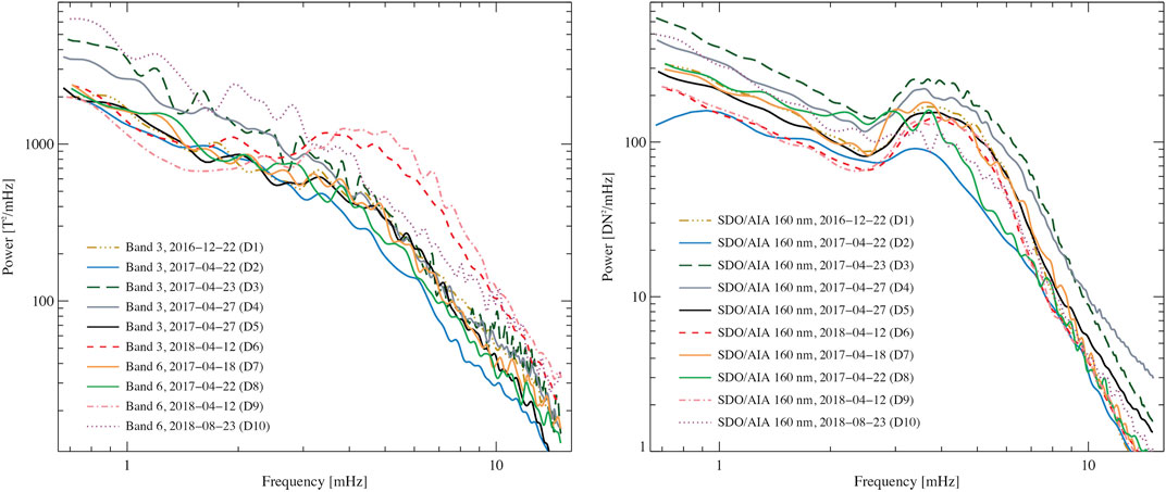
FIGURE 1. Mean power spectra from 10 ALMA datasets (averaged over the entire FOVs) observed in Band 3 and Band 6, sampling the mid-to-upper chromosphere (left) and from their lower chromospheric counterparts observed with SDO/AIA in 1600 Å (right). Images reproduced from Jafarzadeh et al. (2021).
Jafarzadeh et al. (2021) additionally calculated magnetostatic potential field extrapolations from photospheric magnetic fields simultaneously observed with the SDO’s Helioseismic and Magnetic Imager; (HMI Schou et al., 2012). From the extrapolations, the magnetic topologies associated with the areas observed by ALMA could be inspected. Figure 2 shows observations and calculations for a contrasting pair of such Band 3 observations. For each dataset we show the ALMA brightness temperature map (panels a, e), spatially averaged power spectra (panels b, f), corresponding HMI magnetogram associated to a larger FoV compared to that of ALMA (panels c, g), and a top view of the field topology above the ALMA FoV at upper chromospheric heights (panels d, h). The averaged power spectra are shown from two different spectral analysis methods, Fast Fourier Transform (FFT; Cooley and Tukey 1965) and Lomb-Scargle approach (Lomb, 1976; Scargle, 1982). The latter is particularly relevant since the ALMA observations have a 2–3 min gap between blocks of
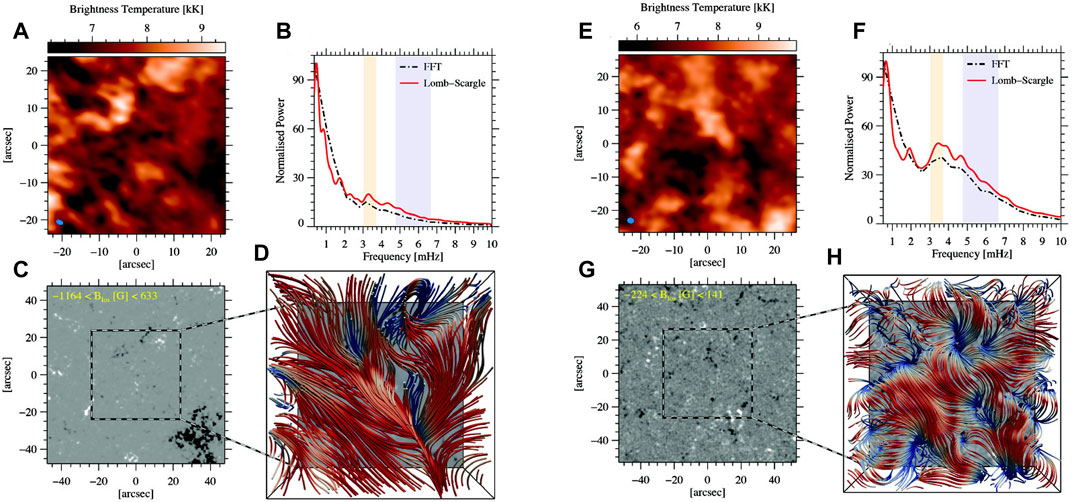
FIGURE 2. Panels (A–D): the 22 December 2016 Band 3 dataset used for the detection of mm-λ oscillations. (A) An ALMA brightness temperature map in Band 3. (B) Spatially averaged brightness temperature power spectra from FFT (dash-dotted black line) and Lomb-Scargle (solid red line) transforms. Period ranges corresponding to the 3 and 5 min windows (each with a width of 1 min) are respectively depicted with the purple and yellow stripes. (C) The SDO/HMI line-of-sight photospheric magnetogram for a FOV twice as large as ALMA’s. The ALMA’s FOV is marked with the dashed square. (D) A top view of the field topology at upper chromosphere heights above the ALMA’s FOV. The colors identify inclination angles, from vertical (blue) to horizontal (red). Panels (E–H): same as panels (A–D) but for the 12 April 2018 Band 3 dataset. Figure reproduced from Jafarzadeh et al. (2021).
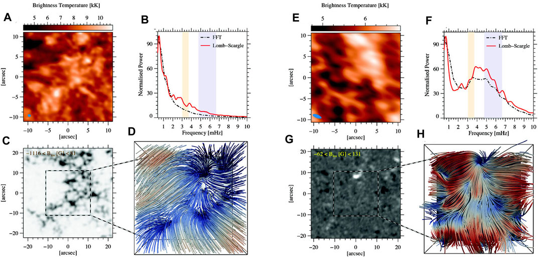
FIGURE 3. Same as Figure 2 but for the 22 April 2017 Band 6 dataset (panels A–D) and the 12 April 2018 Band 6 dataset (panels E–H). Figure reproduced from Jafarzadeh et al. (2021).
The importance of magnetic field environment in observation of p-modes in the mid-to-upper chromosphere (sampled by the ALMA Band 3 and 6 observations) may better be understood when the datasets appearing in Figure 2 for Band 3 and Figure 3 for Band 6, are compared. As evidenced in Figures 2A–D, the photospheric counterpart of the ALMA observations samples a very quiet region, while a strong enhanced-network patch in its immediate vicinity (the lower-right corner) creates the overarching highly inclined magnetic canopy over the entire FoV at the heights sampled by ALMA Band 3. As a result, the averaged power spectrum does not show any power enhancements at around 3–5 mHz. In comparison, when both the ALMA FoV and its surroundings pose very quiet areas in the photosphere (Figures 2E–H), the magnetic topology at chromospheric heights is organized in smaller-scale and less dense loops compared to those rooted in strong kG fields. Thus, the p-modes are not fully obscured, resulting in power enhancements in the 3–5 mHz frequency range. The first example shown in Figures 3A–D for ALMA observations in Band 6 refers to a plage area in both ALMA FoV and its surroundings, as illustrated in the HMI magnetogram. Hence, both nearly vertical fields and a dense magnetic canopy can be observed at the heights sampled by the ALMA Band 6. On the other hand, the p-modes show well in the other Band 6 dataset presented in Figures 3E–H which corresponds to the same target that was presented in Figures 2E–H.
The absence of power enhancements around 3–5 mHz (thus, lack of p-mode detection) could be the result of a combination of various phenomena. In the magnetic canopy regions, both the “umbrella” effect, where the magnetic canopy obscures oscillations coming from lower heights, and possibly the large field inclination angles (Heggland et al., 2011) could be responsible for the absence of p-mode observations. In addition, in the strong field concentrations, where the field is nearly vertical at chromospheric heights, acoustic power suppression (known as “magnetic shadows”; Leighton et al., 1962; Title et al., 1992) may develop due to multiple wave-mode conversions at the plasma-β ≈ 1 level(s), where interactions between p-mode oscillations and the embedded magnetic fields occur (Moretti et al., 2007; Nutto et al., 2012).
2.1.2 Properties of p-mode oscillations
Patsourakos et al. (2020) and Nindos et al. (2021) analyzed spatially-resolved observations of p-mode oscillations in the quiet Sun and deduced their physical characteristics. This was achieved by analysis of the spatially averaged Power Spectral Density (PSD) either for the entire observed FoV or by employing appropriate spatial masks for the cell and network separately. The resulting PSDs for frequency windows encompassing the p-mode peaks were fitted by the sum of a linear and log-normal function of the logarithm of frequency meant to reproduce the background and p-mode peak, respectively. From the log-normal part of the fitting function, the p-mode frequency, amplitude and width were deduced.
In Patsourakos et al. (2020) Band 3 quiet Sun observations with a spatial resolution of typically 2.5″ × 4.5″ and a 2-s cadence were analyzed. The employed FoVs were 80″ × 80″ and scanned quiet Sun targets from disk center to the limb. Spatially resolved chromospheric oscillations with frequencies of 4.2 ± 1.7 mHz were detected in both cell and network. While individual pixels exhibited brightness temperature fluctuations of up to a few hundred K, the spatially averaged PSDs corresponded to fluctuations in the range 55–75 K, which amounts up to the 1% of the spatio-temporal averaged brightness temperature. A moderate increase of the relative p-mode strength (i.e., root mean square, rms, brightness temperature divided by the average brightness temperature) from disk center to limb was also registered.
In Nindos et al. (2021) a quiet Sun region near disk center was observed at both Band 6 and Band 3 at a 1-s cadence. The spatial resolution (FoV) was 1″, 2″ (30″ × 30″, 60″ × 60″), for Band 6 and Band 3, respectively. The resulting PSDs are given in Figure 4. In both bands, p-mode oscillations with frequencies in between 3.6 and 4.4 mHz were found with amplitudes of 103 and 107 K for Band 6 and Band 3, respectively. The associated relative brightness temperature fluctuations with respect to the spatio-temporal average of the brightness temperature were 1.7–1.8%. Bringing the superior
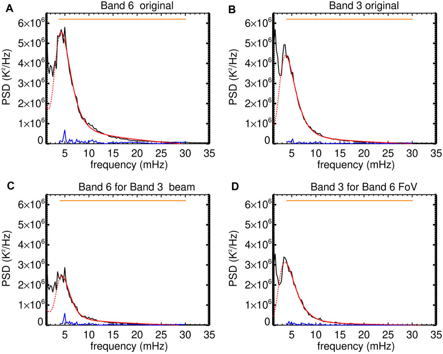
FIGURE 4. Quiet-Sun p-mode oscillations observed at 3 and 1.25 mm by ALMA. Black lines correspond to the spatially averaged PSDs, red lines to their fittings, and blue lines to the absolute residuals between the observed PSDs and the associated fittings. Panels (A,B) correspond to the original Band 6 and Band 3 observations, panel (C) to Band 6 observations at Band 3 spatial resolution and panel (D) for Band 3 observations corresponding to the Band 6 FoV (from Nindos et al., 2021). Reproduced with permission © ESO.
The p-mode oscillations corresponded to the 0.5–0.6 of the spectrum-integrated power (i.e., PSD integral over the entire considered frequency range), which suggests they correspond to a significant fraction of the observed brightness temperature fluctuations. On the other hand, the energy density of the p-mode oscillations in Band 6 was about 3 × 10⁻² erg cm−3, which is roughly equivalent (see Nindos et al., 2021, for details) to a power per unit area that is about an order of magntitude smaller than the energy losses of the quiet chromosphere.
Comparing with previous mm-λ quiet Sun observations at 3.5 mm at a spatial resolution of 10″ with Berkeley- Illinois-Maryland (BIMA) presented by White et al. (2006) and Loukitcheva et al. (2006), the ALMA observations discussed above, due to their superior spatial resolution, allowed, for the first time, to spatially resolve cell and network oscillations and also to deduce higher oscillation amplitudes.
2.2 High-frequency oscillations
High-frequency oscillations are of particular importance since they can carry a vast amount of energy to the upper solar atmosphere. Such waves, of different magneto-acoustic (magnetohydrodynamic) types, have previously been observed in the ultraviolet to infrared wavelength range and have shown to be energetic enough to potentially heat the solar chromosphere and beyond (De Pontieu et al., 2007a; Kuridze et al., 2012; Kubo et al., 2016; Jafarzadeh et al., 2017c; Gafeira et al., 2017). However, in the pre-ALMA era most studies, with an exception of that by Okamoto and De Pontieu (2011), have not identified high-frequency waves in the upper chromosphere. Only recently, such high-frequency oscillations have also been detected at millimeter wavelengths, thanks to high-quality observations provided by ALMA. As such, Guevara Gómez et al. (2021) studied the dynamics of small-scale bright features observed with ALMA Band 3 (supposedly sampling heights that correspond to the upper chromosphere). They found that the majority of their small, likely magnetic, structures exhibit oscillations in brightness temperature, size, and horizontal motion, with periods on the order of 90 ± 22 s, 110 ± 12 s, and 66 ± 23 s, respectively.
Recent publications have begun investigating properties of high-frequency oscillations and p-modes at millimeter wavelengths in the solar chromosphere, using state-of-the-art numerical simulations (Eklund et al., 2021b). However, Fleck et al. (2021) showed that such numerical models should be treated with great caution. They compared various simulation codes and found that the height dependence of wave power, particularly for high-frequency waves, varied between the models by up to two orders of magnitude.
2.3 Sunspot oscillations
Sunspot oscillations are one of the most well known oscillatory phenomena in the solar atmosphere. The oscillations are detected as intensity and velocity variations (e.g. see the review by Khomenko and Collados, 2015, and references therein). In the umbra, at photospheric heights, oscillations with periods in both the 5-min range and the 3-min range have been established. Higher up in the chromosphere, oscillations with periods of 150–200 s exhibit larger amplitudes and are detected in the inner part of the umbra. Sunspot oscillations are directly linked with the propagation of MHD waves. The 5-min oscillations are thought to be driven by the p-modes while the traditional interpretation of the 3-min oscillations considered them as produced by a resonant cavity provided by the sunspot itself (e.g. see Bogdan and Judge, 2006; Khomenko and Collados, 2015; Jess et al., 2020). Detection of such chromospheric resonances appears to be challenging (Felipe, 2021) and may depend on the spatial resolution and quality of observations (Jess et al., 2021). It has also been advocated that the 3-min oscillations indicate upward-propagating waves that pass through the gravitationally stratified gas (Felipe et al., 2010; Chae and Goode, 2015). The sunspots’ magneto-acoustic oscillations in the solar chromosphere are also responsible for observable changes in coronal plasma composition (Baker et al., 2021; Stangalini et al., 2021).
Using ALMA 3 mm observations, Chai et al. (2022) reported the first detection of spatially resolved 3-min oscillations of the mm-λ emission above the umbra of a sunspot. The detected modulation of the mm-λ emission is linked to the temporal variability of the chromospheric electron temperature through the free-free emission. These authors calculated the spatial distribution of the 3-min power amplitude (see Figure 5) which correlated well to similar maps made from observations at several locations along Hα line except at +0.8 Å where the oscillatory power was weak. From the 3-mm and Hα time profiles they found that there was a rather constant phase offset among ALMA brightness temperature and Hα sub-band intensities. Comparison of the properties of the mm-λ oscillations with the acoustic hydrodynamic model by Chae and Goode (2015) revealed that the ALMA intensity fluctuations were consistent with the propagation of an acoustic wave above the umbra. Furthermore, the 3-mm oscillations exhibited a slower rise and faster fall which may indicate nonlinear wave steepening or shock behavior above the umbra.
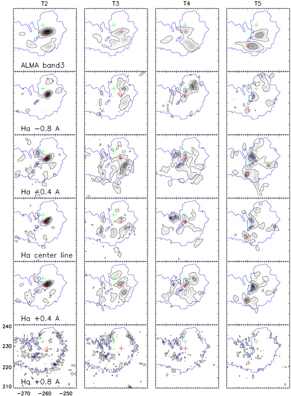
FIGURE 5. Spatial distribution of the 3-min oscillation power amplitude in 3 mm (top row) and in various sub-bands along the Hα line. The columns correspond to different ALMA solar scans, each of duration of about 10 min (from Chai et al., 2022). © AAS. Reproduced with permission.
3 Weak transient activity
3.1 Statistical properties of transient brightenings
In addition to oscillations, several studies have reported transient brightenings in both quiet Sun (Yokoyama et al., 2018; Eklund et al., 2020; Nindos et al., 2020, 2021) and active region (Shimojo et al., 2017b; da Silva Santos et al., 2020; Chintzoglou et al., 2021b; Shimizu et al., 2021) observations with ALMA. In relation to the ALMA frequencies used, most of these reports utilize Band 3 observations with the exception of the papers by Nindos et al. (2021) who presented both Band 3 and Band 6 observations and Chintzoglou et al. (2021a) who analyzed Band 6 data. No observations in Band 7 (0.86 mm) recently made available for solar observing have been published thus far.
Obviously, any meaningful statistics of the properties of such events requires their detection in sufficient numbers. Large numbers of events have indeed been reported by Nindos et al. (2020, 2021), and Eklund et al. (2020). These authors analyzed ALMA quiet Sun data and the identification of their events resulted from the application of algorithms designed for that purpose. Nindos et al. (2020, 2021) applied intensity and temporal thresholds to the light curves of all pixels after they removed the effect of p-mode oscillations (see section 2.1.2). The resulting active pixels were further constrained by applying a spatial clustering criterion determined by the size of the ALMA beam and combined with a synchrony tolerance of ±2 min between time profile peaks of the selected adjacent pixels. Eklund et al. (2020) searched for intensity peaks in excess of 400 K in the light curves of all pixels. Then the selected pixels were grouped together by employing a k-means clustering algorithm.
Nindos et al. (2020) detected a total of 184 3-mm transient events in six quiet Sun regions located from close to the limb to disk center (Nindos et al., 2018), each one observed for about 10 min. Nindos et al. (2021) detected 77 and 115 events at 1.25 and 3 mm, respectively, in a very quiet region that was observed close to disk center for about 40 min. These numbers correspond to occurrence rates per unit area of about [2–5] × 10–22 events per cm2 s. However, the number of ALMA events with AIA counterparts (either at 1600 or 304 Å) was about 6–10 times smaller (see Figure 6). This might be due to the different temperature ranges sampled by the ALMA-AIA datasets with the ALMA events probing cooler material whose temperature increase may not be sufficient to give rise to emission in the 304 Å passband. On the opposite side, the AIA events may be rather weak to energize the layers probed by ALMA. Furthermore all ALMA-AIA events in these studies should be optically thick and since 3 mm emission must be coming from higher layers than 1600 Å (Howe et al., 2012; Alissandrakis et al., 2017; Patsourakos et al., 2020), it is not surprising that the higher 3-mm transients do not correlate well with the 1600-Å transients that appear lower down because, at 3 mm, we cannot see down to those heights.
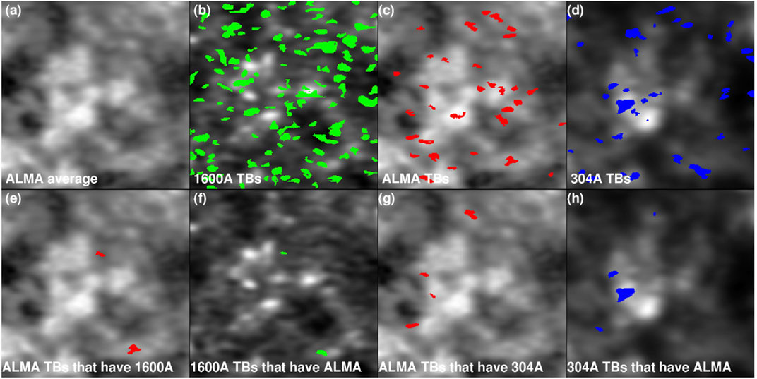
FIGURE 6. The different colors mark the pixels participating in transient brightenings in 1600 Å (green), 3 mm (red) and 304 Å (blue) 10-min data of a quiet Sun region. In panels (A–D) all events identified at a given wavelength are displayed. In the bottom row, panels (E,F) display the events appearing both at 3 mm and 1600 Å while panels (G,H) display the events appearing both at 3 mm and 304 Å (from Nindos et al., 2020). Reproduced with permission © ESO.
The events detected by Nindos et al. (2020, 2021) exhibited brightness temperature increases from ∼40 K to more than 500 K above background levels. Most of them were weak; for example the 3-mm event of Figure 7 can be detected only after the average image is subtracted from each snapshot (compare panels of rows (a) and (b)). They were all of the gradual rise-and-fall type (see the bottom panel of Figure 7 for a characteristic example) with mean durations (quantified by the FWHM of the event’s light curves) of about 50 s. The gradual nature of the light curves suggests the events result from thermal free-free emission (e.g. see Nindos, 2020). Although the presence of nonthermal electrons has been reported in previous studies of microwave transient brightenings (e.g. Gary et al., 1997; Krucker et al., 1997; Nindos et al., 1999), model calculations (White and Kundu, 1992) indicate that one needs to invoke a population of MeV-emitting electrons to obtain appreciable gyrosynchrotron emission at 1–3 mm. We also note that Nindos et al. (2020, 2021) found power-law behavior for the maximum intensity, duration, and size of their brightenings with indices in the interval of 1.93–3.11 which is broadly consistent with those for EUV transient brightenings (e.g. see Joulin et al., 2016, and references therein).
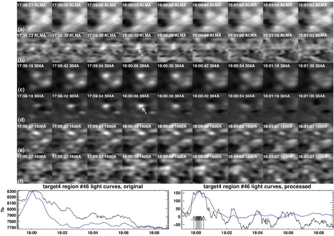
FIGURE 7. A quiet Sun transient event observed at 3 mm and 304 Å. Panel (A) shows characteristic ALMA snapshots while panel (B) shows the same snapshots after the average 3 mm image has been subtracted. Rows c–f: same as (A,B) but for the 304 (C,D) and the 1600 Å data (E,F). The white arrows mark the transient brightening. The field of view is 35″ × 35″. Bottom row: light curves of the event emission at 3 mm (black) and 304 Å (blue) before and after processing (left and right panel, respectively) (from Nindos et al., 2020). Reproduced with permission © ESO.
Eklund et al. (2020) detected 552 3-mm events in a quiet region that was observed for about 40 min (Wedemeyer et al., 2020). The occurrence rate per unit area of these events was almost two orders of magnitude larger than those reported by Nindos et al. (2020, 2021). This discrepancy could be interpreted in terms of either possible intrinsic differences among the regions considered or differences in the detection algorithms (for example Eklund et al., 2020, might have not removed oscillations prior to the application of their search criteria).
It is worth mentioning that the number of ALMA detected events in the publications mentioned above could be considered as lower limits to their actual numbers due to smearing introduced to the data by the finite spatial resolution (see Eklund et al., 2021b), thus leaving some of the weak events undetectable. The simulations performed by Eklund et al. (2021b) indicate that the situation improves as spatial resolution becomes better; therefore it is advisable to search for weak transient brightenings using the wider ALMA array configurations.
In contrast to the events discussed above, the active-region transient events studied by da Silva Santos et al. (2020) were EUV-selected, i.e. they were first identified in AIA EUV images and then their 3 mm counterparts were detected in ALMA data. da Silva Santos et al. (2020) reported the detection of nine transient ALMA events in a field of view of 60″ throughout their 60-min observing run. Their occurrence rate per unit area is about two to eight times higher than the occurrence rate per unit area of the ALMA-AIA paired events that were registered by Nindos et al. (2020, 2021).
In the above studies, the locations of the ALMA transients show diversity which is related to different properties of the target regions. The 3 mm events detected by Nindos et al. (2020, 2021) show a weak tendency (about 70%) to appear at the boundaries of network cells in agreement with the visual inspection of Figure 6C. The situation is somehow different in the 1.25 mm events detected by Nindos et al. (2021) where more than half of the events are located in internetwork regions. This difference is a natural consequence of the fact that much of the field of view of the 1.25 mm observations by Nindos et al. (2021) was covered by the interior of a supergranular cell whereas that was not the case for the 3-mm observations by Nindos et al. (2020, 2021).
The quiet Sun events detected by Eklund et al. (2020) show a tendency to occur in regions of lower magnetic field strength. This is obvious in Figure 8 where the white spaces of panel (b) that are not associated with any events correspond to the stronger magnetic field concentrations that appear in panel (a). This was one of the arguments used by Eklund et al. (2020) to interpret the origin of their events in terms of propagating shock waves (see Section 3.4).
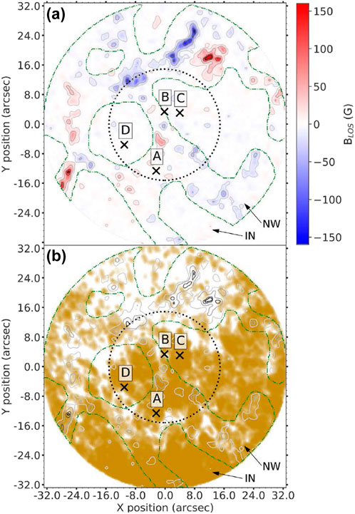
FIGURE 8. (a) HMI magnetogram of a quiet Sun region with the magnetic field displayed in gray contours as well as blue, white, and red shades. The green dashed-dotted curves distinguish network regions from internetwork regions. The dotted circle marks the 30″-diameter region whose transients were analyzed. (b) The color marks the pixels participating in transient events with a brightness temperature
The region studied by da Silva Santos et al. (2020) was centered at a group of pores in the periphery of a large sunspot (see Figure 9); part of that region was the site of magnetic flux emergence during the ALMA observations. These authors identified Ellerman bombs in their 1700 Å AIA data but did not find any conspicuous brightenings associated with them in the ALMA data. This result may indicate that Ellerman bombs are reconnection events that are formed at heights around temperature minimum (e.g. see Georgoulis et al., 2002; Archontis and Hood, 2009; Watanabe et al., 2011; Hansteen et al., 2019), that is, well below the formation height of the 3-mm continuum emission. It appears that ALMA 0.86 mm observations that may probe lower heights than Band 6 might be more appropriate to search for mm-λ counterparts of Ellerman bombs.
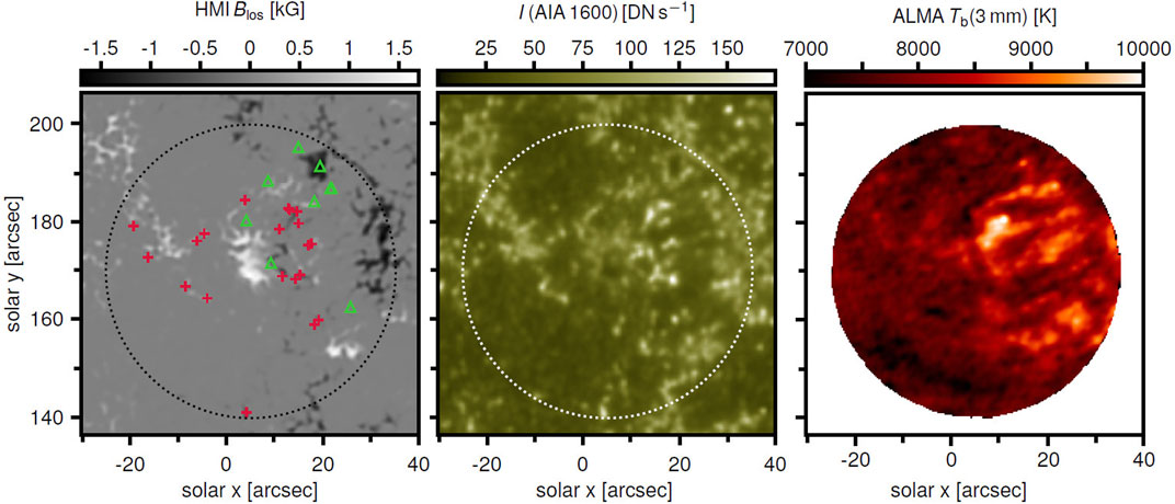
FIGURE 9. A small active region observed by SDO and ALMA. The left image is a longitudinal magnetogram from HMI/SDO, the middle image has been obtained by AIA/SDO while the right image shows the ALMA 3 mm emission. The dotted circles show the ALMA field of view. In the magnetogram the crosses mark the locations of Ellerman bombs. The triangles indicate locations of transient brightenings detected by both AIA and ALMA (adapted from da Silva Santos et al., 2020). Reproduced with permission © ESO.
Contrary to the null detection of Ellerman bombs, da Silva Santos et al. (2020) reported the detection of bright (above 9000 K and up to 14,200 K corresponding to excess emissions of up to ∼5000 K above background) 3-mm events that were better correlated with transient EUV brightenings than UV ones (see Figure 10). This may indicate that these 3 mm-λ brightenings may probe material from the upper chromosphere with overlapping contributions from the transition region and even the corona. Therefore these transients are more reminiscent of the UV bursts identified by Guglielmino et al. (2018), that is small, bright transients occurring higher than the photospheric/low chromospheric layers where the usual small-scale UV active region transient brightenings occur (e.g. see the review by Young et al., 2018, and references therein).
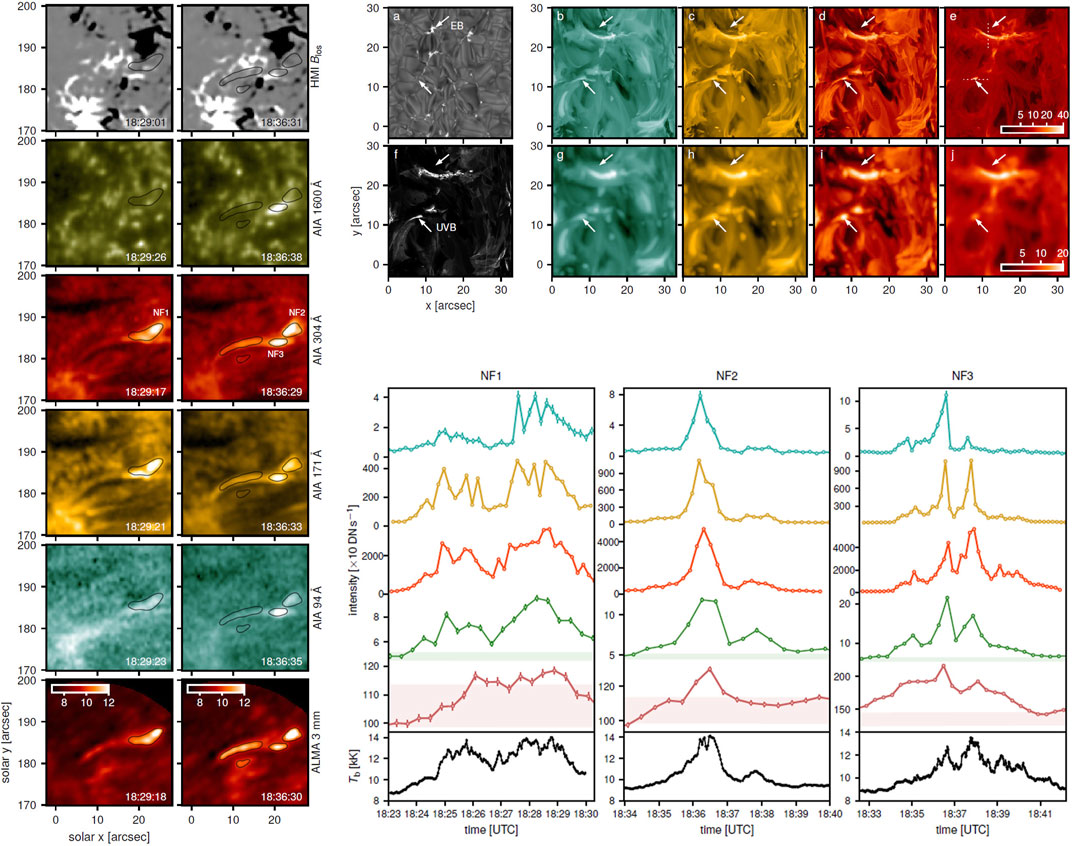
FIGURE 10. The two leftmost columns show characteristic snapshots of flaring fibrils in an HMI magnetogram, several AIA channels and ALMA 3 mm data. The contours mark a 3-mm brightness temperature of 104 K. The two rows at the top-right part of the figure show results from an r-MHD simulation. Panels (A,F) show Hα line wing and integrated Si IV 1393 Å intensity while panels (B–E) show the simulation’s emission in AIA 94, 171, 304 Å and 3 mm, at its original spatial scale. In panels (G–J) the spatial resolution of the simulation has been degraded resulting to pixel size of 0.3″. The top and bottom arrows mark the locations of an Ellerman bomb and a UV burst, respectively. The remaining columns at the bottom-right part of the figure show time profiles (3 mm, 1700, 1600, 304, 171, and 94 Å from bottom to top) of the events marked NF1, NF2, NF3 at the two left columns (adapted from da Silva Santos et al., 2020). Reproduced with permission © ESO.
3.2 Morphology of transient activities
Most studies of ALMA transient brightenings have come out of observations obtained with a 3-mm spatial resolution of
The first detection of a resolved transient brightening has been reported by Shimojo et al. (2017b) (see Figure 11 for a snapshot around the peak of the event). The event was associated with an X-ray bright point near a sunspot. The bright point was visible in soft X-ray, EUV, and 3-mm images. The location of the brightest part of the 3-mm source (left box of the top left panel of Figure 11) matches the loop top of the X-ray bright point. Hence, it is hard to think that the 3-mm source is located in the chromosphere, and the source might not be optically thick.
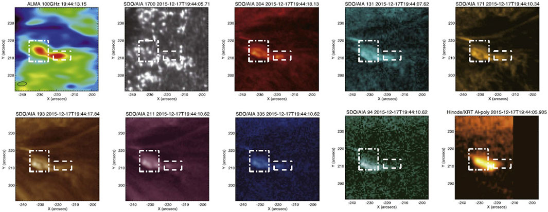
FIGURE 11. Images of a plasmoid ejection close to the time of its maximum emission. From left to right and top to bottom we present images at 3 mm (ALMA), 1700, 304, 131, 171, 193, 211, 335, and 94 Å (all from AIA), and Al-poly filter soft X-rays (from Hinode XRT) (from Shimojo et al., 2017b). © AAS. Reproduced with permission.
The time evolution of the event in the EUV and soft X-ray images is similar to that of coronal jets (e.g. see Shimojo et al., 2007; Moore et al., 2010; Raouafi et al., 2016). At first, the X-ray bright point flares up, small flare loops are created, and an elongated jet structure develops simultaneously from near the loop top. Then a plasmoid blob ejects from the bright point. Interestingly, the apparent direction of motion of the plasmoid is slightly different from the direction of motion of the jet. In the 3-mm images, emission from both the flaring bright point and the plasmoid can be seen (see Figure 11). Shimojo et al. (2017b) argued that the plasmoid was neither a chromospheric object nor was it optically thick. Their analysis indicated that the plasmoid consisted either of isothermal
Transient ejecta have also been revealed in other ALMA observations. For example Yokoyama et al. (2018) presented the ejection of a small blob at 3 mm which was associated with a spicule appearing in Mg II images obtained with the Interface Region Imaging Spectrograph (IRIS De Pontieu et al., 2014). This may suggest a relationship between the ejection of plasmoids and the development of spicules. We note that the mm-λ emission from solar structures mainly arises from continuum processes (see Section 1). Therefore even when the velocity of the emitting structure increases rapidly, we will still be able to track its motion in contrast to what might happen in spectral line observations due to their narrow band-pass. In this respect, ALMA images may serve as a valuable tool for tracing ejecta.
We note in passing that Yokoyama et al. (2018) also revealed that there is a correspondence in the solar limb location between 3-mm ALMA images and 171 Å images obtained by AIA/SDO. Since the limb is populated by dynamic structures like spicules, this result can be used both for the coalignment of ALMA and EUV images and for constraining the variation of their density with height.
Figure 10 indicates that some of the events detected by da Silva Santos et al. (2020) (see Section 3.1) were also resolved and showed an elongated shape bridging regions of opposite magnetic polarities and exhibiting proper motions with high apparent velocities (37–340 km s−1). da Silva Santos et al. (2020) compared their results with a snapshot from a radiative MHD (r-MHD) simulation of magnetic flux emergence (see top part of right column of Figure 10). The simulation region contained an Ellerman bomb and an UV burst marked by the top and bottom arrows in panels (a)-(j), respectively. In agreement with the observations there is no signature of the Ellerman bomb in the simulated 3-mm emission but the presence of the UV burst, probably a signature of magnetic reconnection following flux emergence, is captured as a rather elongated structure in good qualitative agreement with the UV and 3-mm observations that appear in the left column of Figure 10.
3.3 Energetics of transient brightenings
The importance of transient brightenings as potential contributors to the heating of the upper layers of the solar atmosphere has been highlighted in Section 1. Therefore it is not a surprise that in some of the papers reporting on ALMA transient brightenings, estimates of their energy content are provided. The mm-λ emission is considered to arise from thermal free-free emission. Three approaches to the subject have been developed: 1) Direct use of the ALMA brightness temperature enhancements for the calculation of the thermal energy supplied to the chromosphere by the transients (Nindos et al., 2020, 2021; Shimizu et al., 2021). 2) Combine ALMA data with EUV or soft X-ray data to constrain the temperature and density of the event’s plasma and then use these results to estimate its thermal energy content (Shimojo et al., 2017b). 3) Calculate heating rates from a pertinent MHD simulation and compare the results with ALMA observations (da Silva Santos et al., 2022a).
In approach 1) the mm-λ brightness temperature enhancement is considered to be equal to the electron temperature increase of the plasma which is correct only if the mm-λ emission is optically thick. Nindos et al. (2020, 2021) and Shimizu et al. (2021) used the electron temperature values resulted from invertions of center-to-limb variation curves performed by Alissandrakis et al. (2017, 2020) with the corresponding model densities from pertinent Fontenla et al. (1993) models and verified that that was indeed the case in their events. In these studies it was assumed that the density did not change during the events and was taken from models (Fontenla et al., 1993; Loukitcheva et al., 2015). That is a rather crude treatment of the problem which, however, is justified by the lack of appropriate data to perform differential emission measure (DEM) analysis.
Nindos et al. (2020, 2021) found that the thermal energies of their transient brightenings ranged from
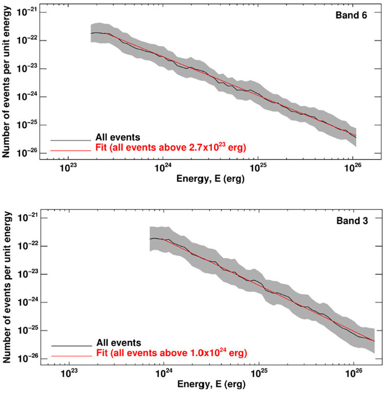
FIGURE 12. Energetics of quiet Sun ALMA transients. In the top panel, the black curve outlines the frequency distribution of 1.25-mm transients. The gray band marks the uncertainties while the red line represents the power-law fit (with index of 1.64) of the frequency distribution for energies
Shimizu et al. (2021) performed an in-depth analysis of a microflare event observed at 3 mm as well as in UV, EUV, and soft X-rays. The thermal energy supplied to the chromosphere by the event was 2.2 × 1024 erg. This estimate was derived from the 3 mm emission at the footpoint of a (micro-)flaring loop that emitted in soft X-rays. The soft X-ray data were used to estimate the event’s thermal energy that was supplied to the corona. It was found that the coronal excess energy was about 100 times larger than the chromospheric one. The fact that compared to the soft X-ray emission, the event’s emission at 3 mm was 1) more impulsive, 2) clearly reached its peak before the soft X-ray emission, and 3) was associated with a microflare’s footpoint while the soft X-ray emission came from the loop led Shimizu et al. (2021) to argue that the energy measured from the 3 mm data can be viewed as a proxy to the energy carried by the non-thermal electrons that impinge deeper and denser atmospheric layers. This result may reflect that the non-thermal energy is not adequate to account for the thermal component in this event because of a deficit of such energetic electrons. Warmuth and Mann (2020) reached a similar conclusion for a set of weak flares they analyzed.
When an event’s mm-λ emission is optically thin, the observed excess brightness temperature is not equal to the plasma electron temperature increase. In such case if the event has been co-observed in EUV or soft X-rays, the variation of the assumed electron density and temperature may reveal parameter spaces that can reconcile the intensity enhancements in both EUV/soft X-rays and mm-λ. That was the strategy adopted by Shimojo et al. (2017b) who found that in their plasmoid event (see Section 3.2) the appropriate pair of electron temperature and density (105 K and 3 × 109 cm−3, respectively) yields a thermal energy of 5 × 1024 erg.
An alternative, albeit less straightforward approach, is to constrain the energetics of mm-λ transient events by comparing their observations with MHD simulations. This path was followed by da Silva Santos et al. (2022a) who found enhanced heating rate of up to 5 kW m−2 in the upper chromosphere part of a simulation box that contained small emerging loops interacting with the overlying canopy field in a situation that resembles the events studied by da Silva Santos et al. (2020) (see also Figure 10). The simulation reproduced well the observations and indicated that the observed 3 mm brightness temperature may form as a weighted average of significant contributions from different layers along the line of sight (see Martínez-Sykora et al., 2020).
3.4 Detection of shock waves
Significant attention has been drawn to the detection of possible signatures of propagating shock waves in ALMA data because: 1) dissipation of shock waves may have a bearing on the heating of the chromosphere and corona, and 2) 1D hydrodynamic simulations (see Loukitcheva et al., 2004, 2006) as well as 3D radiative MHD simulations (see Wedemeyer-Böhm et al., 2007; Loukitcheva et al., 2015; Eklund et al., 2020, 2021a, and also the review by Wedemeyer et al. included in this special Research Topic collection) have revealed that the signatures of such shocks could be identified in ALMA data.
Typically, snapshots from 3D simulations of propagating shock waves show, especially in regions of small magnetic field strength, a pronounced small-scale mesh-like pattern of elongated structures which is produced by propagating shock waves. Wedemeyer et al. (2016) (see also Wedemeyer-Böhm et al., 2007) concluded that the larger building blocks of such pattern can still be visible at a spatial resolution of 0.9″. However, such resolution, although feasible with ALMA at 1.25 mm, is probably at or beyond the instrument’s capabilities at 3 mm where most of solar observing programs have been executed; the so-far most used Band 3 antenna configuration, C3, yields spatial resolution of
Simulations also show how a number of plasma and radiation macroscopic parameters may change with height and time during the propagation of a shock wave. As an example in Figure 13 (top left panel) we show the gas temperature as a function of time and height at the location of a shock wave detected in the simulations by Eklund et al. (2021a). In the same panel the formation heights at optical depth τ = 1 for two ALMA Band 6 sub-bands (SB1, 1.298–1.309 mm, and SB4 1.204–1.214 mm) are also plotted (see the blue and green circles). It is clear that the ∼1.25 mm emission tracks well the shock front as it propagates from about 1 Mm up to about 1.4 Mm where it decouples from it. Note, however, that the shock front keeps moving upward. The decoupling occurs due to the lower opacities for the 1.25 mm emission at heights above ∼1.4 Mm. Panel (b) of Figure 13 shows the corresponding time profiles of the SB1-SB4 brightness temperatures as well as the associated gas temperature time profiles at heights where τ = 1. The event’s FWHM is 41 s and the shock-related increase of brightness temperature is about 5000 K.
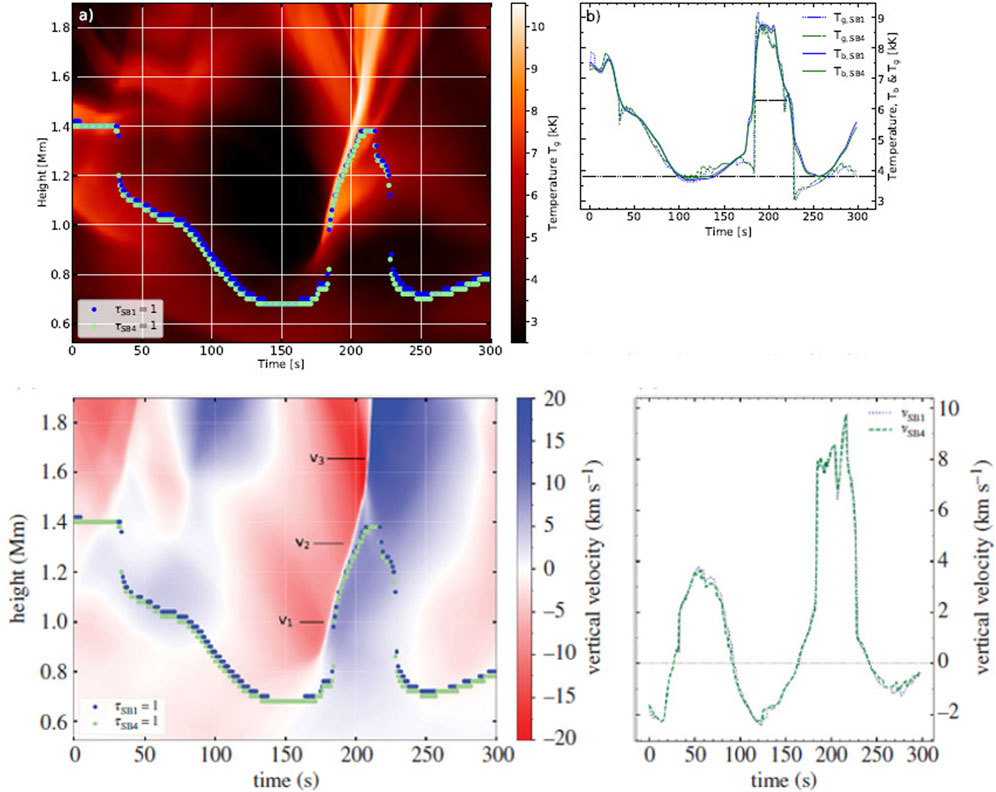
FIGURE 13. Top left [panel (A)]: Gas temperature as a function of time and height for a simulated shock wave. The blue and green dots indicate the formation heights for emission at 1.309 (SB1) and 1.204 mm (SB4), respectively. Top right [panel (B)]: Time profile of the brightness temperature at SB1 (solid blue) and SB4 (solid green) as well as of the gas temperature at the τ = 1 heights of the corresponding wavelengths (blue/green dotted). Bottom panels: same as top panels but for the vertical velocity of the gas (from Eklund et al., 2021a).
In the left bottom panel of Figure 13 we show the material’s vertical velocity associated with the same simulated shock as a function of time and height. The pre-shock region is dominated by a bulk downflow of relatively cool material which is followed by the upflow of hotter material that is associated with the development of the shock. The upflow velocity reaches a value of ∼10 km s−1 at the formation heights of the 1.25 mm radiation but velocities as double as that are registered higher up. On the other hand, the velocity of the vertical propagation of the shock front as can be depicted along the sharp shock-related height-time slopes in the left panels of Figure 13 lies in the range of ∼20–80 km s−1.
The shock-related excess brightness temperature in the simulation we presented in Figure 13 is similar to those reported in other simulations (e.g. see Wedemeyer-Böhm et al., 2007) whereas the transient brightenings detected by Eklund et al. (2020) showed lower excess brightness temperatures up to 1200 K with typical values in the range 450–750 K. However, such discrepancies can be largely reconciled when the simulation results are degraded to the inferior ALMA spatial resolution (see Eklund et al., 2021b). Furthermore, Eklund et al. (2021b) reported that the degraded spatial resolution also affects the lifetime (i.e. FWHM) of shock-related transients because the 3 mm emission is not sensitive to some of the cooler pre-shock material; therefore the ALMA events will tend to be shorter than those detected by simulations. However, these discrepancies (differences on the order of about 15%) should not be as serious as those associated with their brightness temperatures.
Overall, the comparison of the simulation results with ALMA data may lead to the following criteria for the identification of shock signatures in mm-λ transient brightenings (see also Eklund et al., 2020; Chintzoglou et al., 2021b)
• Excess brightness temperature on order from a few hundred to more than a thousand degrees Kelvin.
• Temporal FWHM on the order of tens of seconds.
• Small lateral motions (i.e. with speeds smaller than the local sonic and Alfven speeds) during their lifetime since they are supposed to represent upward-propagating disturbances along magnetic field lines of minimal inclination.
• Occurrence in regions of relatively small magnetic field strength.
• Brightness temperature increases and decreases which should be consistent with undulatory intensity changes recorded in wavelegth-time cuts of the emission from chromospheric lines. This criterion probably provides the most compelling evidence for the presence of a shock wave (see below for the discussion of a particular example).
Eklund et al. (2020) concluded that most of the 552 transients events they detected were consistent with the first four of the criteria listed above (no spectroscopic data were available to them). As an example, in Figure 14 we show one of their best events. The event was largely spatially unresolved, its lifetime was 67 s and the brightness temperature increased by ∼1100 K. Its location corresponds to the cross marked “A” in Figure 8, i.e. it was associated with small magnetic fields. Furthermore, the space-time cuts (panels f–g of Figure 14) yielded an apparent motion of the brightest pixel at the peak of the event (which coincided with the center of the field of view) of about 22 km s−1. This value is somewhat larger that the nominal chromospheric sound and Alfven speeds (which are on the order of ∼10 km s−1, e.g. see Priest, 2014, and references therein) and, in any case, lies toward the high-end limit of the lateral apparent velocities registered by these authors.
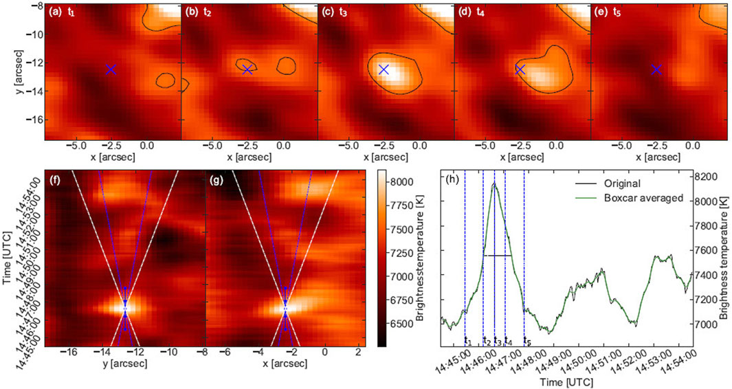
FIGURE 14. Panels (A–E) show characteristic snapshots of a transient brightening attributed to a propagating shock wave. The center of the field of view is marked by the blue “x.” Panels (F,G) show vertical and horizontal cuts, respectively, across the center of the field of view which is indicated by blue dots for the times of panels (A–E). Blue and white lines indicate apparent velocity slopes for 10 and 20 km s−1, respectively. Panel (H) shows the brightness temperature time profile of the center of the field of view (from Eklund et al., 2020). Reproduced with permission © ESO.
When a shock passes through the chromosphere one expects wavelength-time (λ-t) cuts of chromospheric line emission to show a repetitive pattern of a blueshifted excursion that gradually drifts toward the red wing of the line. Such pattern should yield a “sawtooth” modulation in the λ-t cuts. That is exactly what was observed by Chintzoglou et al. (2021b) (see Figure 15) who studied coordinated ALMA 1.25 mm and IRIS UV observations of a plage region. In Figure 15 the time profile of the 1.25 mm emission for the same location of the plage is also displayed; its behavior is similar to the UV wavelength-time drift trends attributed to the propagation of shocks in the chromosphere; note in particular the correlation of 1.25-mm brightness temperature increases and UV blueshifts.
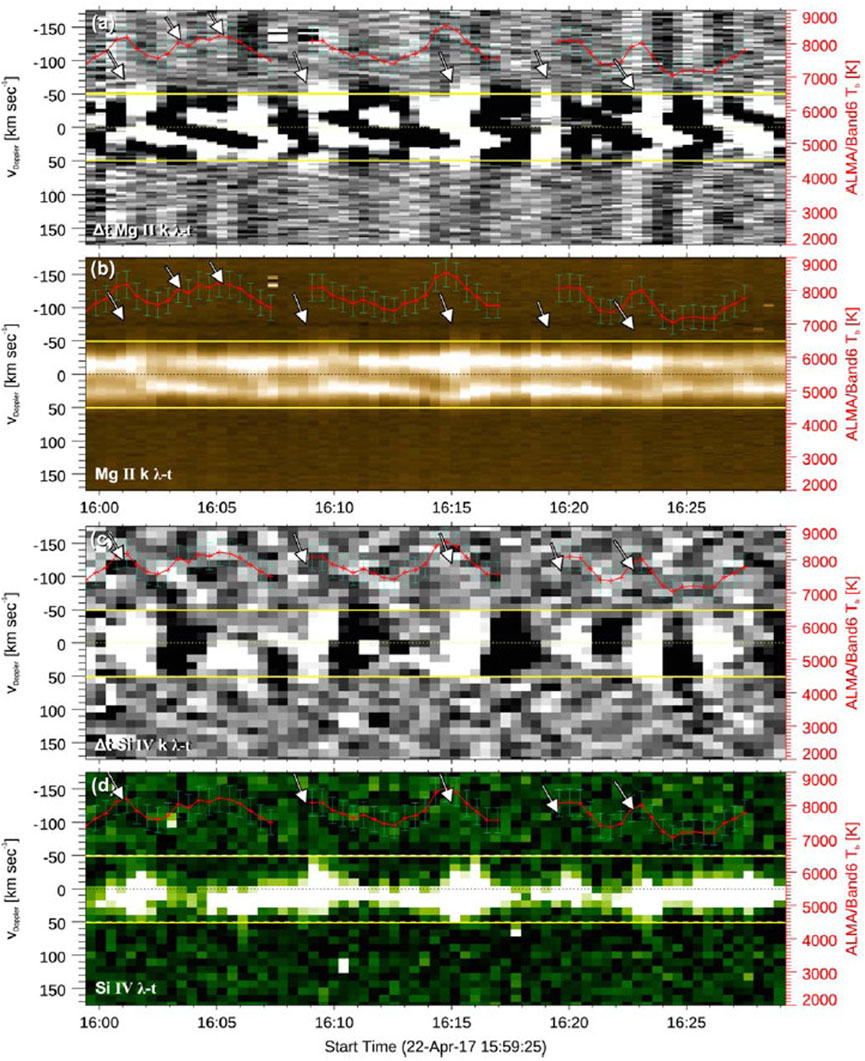
FIGURE 15. Wavelegth-time plot for Mg II k (panel B) and its temporal derivative (panel A) of a 1″ × 1″ area above a plage with recurrent shock waves. Panels (C,D) same as panels (A,B) but for Si IV. In all panels the 1.25 mm emission is overplotted (red curves). The rest-wavelegth position is marked with a dotted line. The arrows point to blueshifts and correlated 1.25-mm emission increases (from Chintzoglou et al., 2021b). © AAS. Reproduced with permission.
Chintzoglou et al. (2021b) concluded that the 1.25-mm plage emission was sensitive to localized heating of the upper chromosphere by propagating shocks. The pertinent brightness temperature jumps were of the order of 10–20% from a reference value of about 7500 K with a decay time of about 60–120 s and a recurrence at about 120 s. This temporal behavior may indicate that multiple shocks from different directions and at different timings could have passed through the specific plage location they considered.
4 Conclusions and prospects for the future
Oscillations, wave phenomena, and transient brightenings, along with turbulence, non-periodic temporal variations, and instrumental noise, all contribute to the observed time variability at any location in the chromosphere. Therefore, for any meaningful study of chromospheric dynamics care must be taken to separate these components. Despite the difficulties several important new results about the dynamic chromosphere have come out since the relatively recent (2016) initiation of regular solar observations with ALMA. The most important findings are summarized below.
• Magnetic field strength and topology largely influence the oscillatory behavior of the chromosphere; the traditional 3-min p-mode oscillations appear at mm-λ only above regions showing small amounts of overlying horizontal magnetic flux, i.e. over weak-field quiet Sun regions.
• When the p-modes are present, they represent brightness fluctuations of about 1–2% with respect to the average quiet Sun. But they correspond to ∼0.5–0.6 of the spectrum-integrated power, i.e. they represent a significant fraction of the observed mm-λ brightness temperature fluctuations. For the first time, their power has been spatially resolved, thanks to the unprecedented ALMA’s spatial resolution. Similar p-mode frequencies have been established both in the network and cell interior.
• High frequency (periods of 66–90 s) oscillations in brightness temperature, size, and horizontal motion of small-scale bright features have been detected for the first time in mm-λ observations.
• The first detection of spatially resolved mm-λ oscillations above a sunspot exhibited properties consistent with the propagation of magneto-acoustic waves above the umbra with some indications of nonlinear steepening.
• A multitude of weak transient brightenings, both in the quiet Sun and active regions, has been detected in ALMA data. Their excess brightness temperature may lie from about 40 K up to about 5000 K above background. Most of them are spatially unresolved. Some of the resolved ones are associated with ejecta that are likely caused by magnetic reconnection.
• The thermal energy of the transient brightenings is between 2 × 10²³ and 1024 erg. The computed lower end of their energy distribution is among the smallest ever reported irrespective of the observing wavelength. However, their power per unit area can account for only ∼1% of the radiative losses from the quiet low chromosphere.
• Brightness temperature increases in mm-λ transient brightenings could result from acoustic/magnetoaccoustic shocks or from magnetic reconnection. Those associated with ejecta are probably induced by reconnection while those showing brightness temperature modulations that are consistent with undulatory intensity changes recorded in λ-t cuts of the emission from chromospheric lines may arise from shocks. A multitude of transients has been attributed to propagating shocks.
The above list highlights ALMA’s great potential to address open issues in chromospheric physics. The major advantage of ALMA data is probably their ability to directly probe the spatial distribution and temporal variability of the electron temperature of the plasma without the need to address complicated effects arising from the non-LTE conditions prevailing in the formation of chromospheric spectral lines.
On the other hand, the major difficulties associated with solar ALMA observations include the small field of view, relatively low spatial resolution compared to state-of-the-art observations in other wavelengths, the availability of a small number of frequency bands, as well as the demanding processing of the visibility data. The field of view can be enlarged by invoking mosaicking techniques at the cost of reduced cadence. With such a setup, only slowly varying phenomena can be tracked and this partly explains why in most of the studies that we reviewed in this paper, Band 3 data were analyzed; it is the frequency band providing the largest FOV, nominally 60″, for solar observing (the other part of the explanation is that, due to weather/atmospheric conditions, the execution of observations becomes increasingly demanding with frequency).
The study of the height dependence of dynamic phenomena requires observations at as many frequencies as possible. Currently ALMA is capable of observing one frequency band at a time. Things will improve by using subarrays, i.e. splitting an array configuration into pieces that observe different frequency bands at the same time or/and by adding new frequency bands to the solar observing programs. For example, the recent addition of Band 7 (0.86 mm) will help us probe lower heights than Band 6. At lower frequencies, a possible future addition of Band 1 (7.25 mm) will probe higher layers where the impact of oscillations should be lower, and thus the detection of weaker transient brightenings could be facilitated. Currently, making snapshot images at different spectral windows within the same ALMA band (see Jafarzadeh et al., 2019; Rodger et al., 2019) could act as a feasible, albeit not completely satisfactory (due to the limited range of sampled heights) alternative, to obtain spectral information about dynamic phenomena. Guevara Gómez et al. (2022b) and also in a work in preparation Guevara Gómez et al. (2022a) have shows that the combination of such spectral windows (to improve the signal-to-noise ratio) at two separate spectral regions within Band 3 yields height separations on the order of 70 km, as well as the approximate determination of propagating speeds of transverse waves identified in ALMA sub-bands and in synthetic data.
Throughout this paper the need for observations with the highest possible spatial resolution has been highlighted because several of the phenomena we discussed (for example transient brightenings) exhibit spatial scales at or below ALMA’s current spatial resolution. Since ALMA’s Cycle 7 (October 2019–October 2021, which includes the observatory’s shutdown period due to the COVID-19 pandemic) the C4 antenna configuration array, whose most extended baseline is over 700 m, has been enabled for solar observations. With the C4 configuration a spatial resolution of about 1″ can be achieved at 3 mm, which constitutes an improvement of a factor of two over the resolution of the Band 3 observations reviewed in this paper. Unfortunately, there has been no paper yet reporting observations of waves or transient events with the C4 configuration. However, the potential to observe with ALMA at sub-arcsecond resolution has been demonstrated by da Silva Santos et al. (2022b) who reported on the fine structure of a filament.
The implementation of circular polarization (Stokes parameter, V) measurements to future solar ALMA observing programs is anticipated to help constraining the magnetic field in the chromosphere. However, we note that the expected low degree of circular polarization outside of active regions demands high sensitivity and will certainly require the development of advanced calibration and imaging procedures. At the time of writing of this paper it is not yet known when solar V ALMA observations will become available. However, synergies between ALMA and high-sensitivity, high spatial and spectral polarimetric observations of photospheric and chromospheric magnetic fields (like the ones that will become available by the Daniel K. Inouye Solar Telescope, DKIST, instrumentation Rimmele et al., 2020) will certainly advance our knowledge on the topics discussed in this paper by shedding light on the upward propagation of waves through the magnetized solar atmosphere and by constraining the magnetic configuration where transient brightenings occur.
We also tried to emphasize that an important ingredient of the recent advances in the study of the dynamic chromosphere is the synergy between the ALMA observations and observations at (E)UV and X-rays. In particular, several spectral lines observed by IRIS (e.g., Mg II h and k) are formed at about the same height as the mm-λ continua observed with ALMA, but probe different plasma properties, thereby providing a highly complementary dataset to the ALMA data (e.g. see Bastian et al., 2017). Last but not least, the coordination of the anticipated sub-arcsecond DKIST and Solar Orbiter (Müller et al., 2020) observations with ALMA has the potential to provide information on the small-scale structure of several chromospheric dynamic phenomena together with their photospheric and transition region counterparts in an unprecentedly long wavelength range from UV to mm-λ.
Author contributions
All authors have contributed to preparing this article.
Acknowledgments
ALMA is a partnership of ESO (representing its member states), NSF (USA) and NINS (Japan), together with NRC (Canada) and NSC and ASIAA (Taiwan), and KASI (Republic of Korea), in co-operation with the Republic of Chile. The Joint ALMA Observatory is operated by ESO, 654 AUI/NRAO, and NAOJ. The National Radio Astronomy Observatory is a facility of the National Science Foundation operated under cooperative agreement by Associated Universities, Inc.
Conflict of interest
The authors declare that the research was conducted in the absence of any commercial or financial relationships that could be construed as a potential conflict of interest.
Publisher’s note
All claims expressed in this article are solely those of the authors and do not necessarily represent those of their affiliated organizations, or those of the publisher, the editors and the reviewers. Any product that may be evaluated in this article, or claim that may be made by its manufacturer, is not guaranteed or endorsed by the publisher.
References
Alissandrakis, C. E., Nindos, A., Bastian, T. S., and Patsourakos, S. (2020). Modeling the quiet Sun cell and network emission with ALMA. Astron. Astrophys. 640, A57. doi:10.1051/0004-6361/202038461
Alissandrakis, C. E., Patsourakos, S., Nindos, A., and Bastian, T. S. (2017). Center-to-limb observations of the Sun with ALMA . Implications for solar atmospheric models. Astron. Astrophys. 605, A78. doi:10.1051/0004-6361/201730953
Archontis, V., and Hood, A. W. (2009). Formation of Ellerman bombs due to 3D flux emergence. Astron. Astrophys. 508, 1469–1483. doi:10.1051/0004-6361/200912455
Baker, D., Stangalini, M., Valori, G., Brooks, D. H., To, A. S. H., van Driel-Gesztelyi, L., et al. (2021). Alfvénic perturbations in a sunspot chromosphere linked to fractionated plasma in the corona. Astrophys. J. 907, 16. doi:10.3847/1538-4357/abcafd
Bastian, T. S., Chintzoglou, G., De Pontieu, B., Shimojo, M., Schmit, D., Leenaarts, J., et al. (2017). A first comparison of millimeter continuum and Mg II ultraviolet line emission from the solar chromosphere. Astrophys. J. 845, L19. doi:10.3847/2041-8213/aa844c
Beckers, J. M., and Schultz, R. B. (1972). Oscillatory motions in sunspots. Sol. Phys. 27, 61–70. doi:10.1007/BF00151770
Beckers, J. M., and Tallant, P. E. (1969). Chromospheric inhomogeneities in sunspot umbrae. Sol. Phys. 7, 351–365. doi:10.1007/BF00146140
Bogdan, T. J., Carlsson, M., Hansteen, V. H., McMurry, A., Rosenthal, C. S., Johnson, M., et al. (2003). Waves in the magnetized solar atmosphere. II. Waves from localized sources in magnetic flux concentrations. Astrophys. J. 599, 626–660. doi:10.1086/378512
Bogdan, T. J., and Judge, P. G. (2006). Observational aspects of sunspot oscillations. Phil. Trans. R. Soc. A 364, 313–331. doi:10.1098/rsta.2005.1701
Carlsson, M., De Pontieu, B., and Hansteen, V. H. (2019). New view of the solar chromosphere. Annu. Rev. Astron. Astrophys. 57, 189–226. doi:10.1146/annurev-astro-081817-052044
Carlsson, M., and Stein, R. F. (2002). Dynamic hydrogen ionization. Astrophys. J. 572, 626–635. doi:10.1086/340293
Carlsson, M., and Stein, R. F. (1992). Non-LTE radiating acoustic shocks and CA II K2V bright points. Astrophys. J. 397, L59. doi:10.1086/186544
Centeno, R., Collados, M., and Trujillo Bueno, J. (2006). Spectropolarimetric investigation of the propagation of magnetoacoustic waves and shock formation in sunspot atmospheres. Astrophys. J. 640, 1153–1162. doi:10.1086/500185
Chae, J., and Goode, P. R. (2015). Acoustic waves generated by impulsive disturbances in a gravitationally stratified medium. Astrophys. J. 808, 118. doi:10.1088/0004-637X/808/2/118
Chai, Y., Gary, D. E., Reardon, K. P., and Yurchyshyn, V. (2022). A study of sunspot 3 minute oscillations using ALMA and GST. Astrophys. J. 924, 100. doi:10.3847/1538-4357/ac34f7
Chintzoglou, G., De Pontieu, B., Martínez-Sykora, J., Hansteen, V., de la Cruz Rodríguez, J., Szydlarski, M., et al. (2021a). ALMA and IRIS observations of the solar chromosphere. I. An on-disk type II spicule. Astrophys. J. 906, 82. doi:10.3847/1538-4357/abc9b1
Chintzoglou, G., De Pontieu, B., Martínez-Sykora, J., Hansteen, V., de la Cruz Rodríguez, J., Szydlarski, M., et al. (2021b). ALMA and IRIS observations of the solar chromosphere. II. Structure and dynamics of chromospheric plages. Astrophys. J. 906, 83. doi:10.3847/1538-4357/abc9b0
Cirtain, J. W., Golub, L., Winebarger, A. R., de Pontieu, B., Kobayashi, K., Moore, R. L., et al. (2013). Energy release in the solar corona from spatially resolved magnetic braids. Nature 493, 501–503. doi:10.1038/nature11772
Cooley, J. W., and Tukey, J. W. (1965). An algorithm for the machine calculation of complex Fourier series. Math. Comput. 19, 297–301. doi:10.1090/s0025-5718-1965-0178586-1
Cram, L. E. (1978). High resolution spectroscopy of the disk chromosphere. VI. Power, phase and coherence spectra of atmospheric oscillations. Astron. Astrophys. 70, 345.
da Silva Santos, J. M., Danilovic, S., Leenaarts, J., de la Cruz Rodríguez, J., Zhu, X., White, S. M., et al. (2022a). Heating of the solar chromosphere through current dissipation. Astron. Astrophys. 661, A59. doi:10.1051/0004-6361/202243191
da Silva Santos, J. M., de la Cruz Rodríguez, J., White, S. M., Leenaarts, J., Vissers, G. J. M., and Hansteen, V. H. (2020). ALMA observations of transient heating in a solar active region. Astron. Astrophys. 643, A41. doi:10.1051/0004-6361/202038755
da Silva Santos, J. M., White, S. M., Reardon, K., Cauzzi, G., Gunár, S., Heinzel, P., et al. (2022b). Subarcsecond imaging of a solar active region filament with ALMA and IRIS. Front. Astron. Space Sci. 9, 898115. doi:10.3389/fspas.2022.898115
De Pontieu, B., Hansteen, V. H., Rouppe van der Voort, L., van Noort, M., and Carlsson, M. (2007a). High-resolution observations and modeling of dynamic fibrils. Astrophys. J. 655, 624–641. doi:10.1086/509070
De Pontieu, B., McIntosh, S. W., Carlsson, M., Hansteen, V. H., Tarbell, T. D., Schrijver, C. J., et al. (2007b). Chromospheric alfvénic waves strong enough to power the solar wind. Science 318, 1574–1577. doi:10.1126/science.1151747
De Pontieu, B., Title, A. M., Lemen, J. R., Kushner, G. D., Akin, D. J., Allard, B., et al. (2014). The Interface region imaging Spectrograph (IRIS). Sol. Phys. 289, 2733–2779. doi:10.1007/s11207-014-0485-y
Eklund, H., Wedemeyer, S., Snow, B., Jess, D. B., Jafarzadeh, S., Grant, S. D. T., et al. (2021a). Characterization of shock wave signatures at millimetre wavelengths from Bifrost simulations. Phil. Trans. R. Soc. A 379, 20200185. doi:10.1098/rsta.2020.0185
Eklund, H., Wedemeyer, S., Szydlarski, M., Jafarzadeh, S., and Guevara Gómez, J. C. (2020). The Sun at millimeter wavelengths. II. Small-scale dynamic events in ALMA Band 3. Astron. Astrophys. 644, A152. doi:10.1051/0004-6361/202038250
Eklund, H., Wedemeyer, S., Szydlarski, M., and Jafarzadeh, S. (2021b). The Sun at millimeter wavelengths. III. Impact of the spatial resolution on solar ALMA observations. Astron. Astrophys. 656, A68. doi:10.1051/0004-6361/202140972
Felipe, T., Khomenko, E., Collados, M., and Beck, C. (2010). Multi-layer study of wave propagation in sunspots. Astrophys. J. 722, 131–144. doi:10.1088/0004-637X/722/1/131
Felipe, T. (2021). Signatures of sunspot oscillations and the case for chromospheric resonances. Nat. Astron. 5, 2–4. doi:10.1038/s41550-020-1157-5
Fleck, B., Carlsson, M., Khomenko, E., Rempel, M., Steiner, O., and Vigeesh, G. (2021). Acoustic-gravity wave propagation characteristics in three-dimensional radiation hydrodynamic simulations of the solar atmosphere. Phil. Trans. R. Soc. A 379, 20200170. doi:10.1098/rsta.2020.0170
Fleck, B., and Schmitz, F. (1991). The 3-min oscillations of the solar chromosphere - a basic physical effect? Astron. Astrophys. 250, 235–244.
Fontenla, J. M., Avrett, E. H., and Loeser, R. (1993). Energy balance in the solar transition region. III. Helium emission in hydrostatic, constant-abundance models with diffusion. Astrophys. J. 406, 319. doi:10.1086/172443
Gabriel, A. H. (1976). A magnetic model of the solar transition region. Philosophical Trans. R. Soc. Lond. Ser. A 281, 339–352. doi:10.1098/rsta.1976.0031
Gafeira, R., Jafarzadeh, S., Solanki, S. K., Lagg, A., van Noort, M., Barthol, P., et al. (2017). Oscillations on width and intensity of slender Ca II H fibrils from sunrise/SuFI. Astrophys. J. Suppl. Ser. 229, 7. doi:10.3847/1538-4365/229/1/7
Gary, D. E., Hartl, M. D., and Shimizu, T. (1997). Nonthermal radio emission from solar soft X-ray transient brightenings. Astrophys. J. 477, 958–968. doi:10.1086/303748
Georgoulis, M. K., Rust, D. M., Bernasconi, P. N., and Schmieder, B. (2002). Statistics, morphology, and energetics of ellerman bombs. Astrophys. J. 575, 506–528. doi:10.1086/341195
Giovanelli, R. G., and Jones, H. P. (1982). The three-dimensional structure of atmospheric magnetic fields in two active regions. Sol. Phys. 79, 267–278. doi:10.1007/BF00146244
Giovanelli, R. G. (1972). Oscillations and waves in a sunspot. Sol. Phys. 27, 71–79. doi:10.1007/BF00151771
Guevara Gómez, J. C., Jafarzadeh, S., Wedemeyer, S., Grant, S. D. T., Eklund, H., and Szydlarski, M. (2022a). The Sun at millimeter wavelengths. IV. Magnetohydrodynamic waves in small-scale bright features. Astron. Astrophys. in prep.
Guevara Gómez, J. C., Jafarzadeh, S., Wedemeyer, S., and Szydlarski, M. (2022b). Propagation of transverse waves in the solar chromosphere through ALMA sub-bands. Astron. Astrophys. 665, L2.
Guevara Gómez, J. C., Jafarzadeh, S., Wedemeyer, S., Szydlarski, M., Stangalini, M., Fleck, B., et al. (2021). High-frequency oscillations in small chromospheric bright features observed with Atacama Large Millimetre/Submillimetre Array. Phil. Trans. R. Soc. A 379, 20200184. doi:10.1098/rsta.2020.0184
Guglielmino, S. L., Zuccarello, F., Young, P. R., Murabito, M., and Romano, P. (2018). IRIS observations of magnetic interactions in the solar atmosphere between preexisting and emerging magnetic fields. I. Overall evolution. Astrophys. J. 856, 127. doi:10.3847/1538-4357/aab2a8
Hansteen, V., Ortiz, A., Archontis, V., Carlsson, M., Pereira, T. M. D., and Bjørgen, J. P. (2019). Ellerman bombs and UV bursts: Transient events in chromospheric current sheets. Astron. Astrophys. 626, A33. doi:10.1051/0004-6361/201935376
Heggland, L., Hansteen, V. H., De Pontieu, B., and Carlsson, M. (2011). Wave propagation and jet formation in the chromosphere. Astrophys. J. 743, 142. doi:10.1088/0004-637X/743/2/142
Henriques, V. M. J., Kuridze, D., Mathioudakis, M., and Keenan, F. P. (2016). Quiet-sun Hα transients and corresponding small-scale transition region and coronal heating. Astrophys. J. 820, 124. doi:10.3847/0004-637X/820/2/124
Hollweg, J. V. (1981). Alfvén waves in the solar atmosphere. Sol. Phys. 70, 25–66. doi:10.1007/BF00154391
Howe, R., Jain, K., Bogart, R. S., Haber, D. A., and Baldner, C. S. (2012). Two-Dimensional helioseismic power, phase, and coherence spectra of solar dynamics observatory photospheric and chromospheric observables. Sol. Phys. 281, 533–549. doi:10.1007/s11207-012-0097-3
Hudson, H. S. (1991). Solar flares, microflares, nanoflares, and coronal heating. Sol. Phys. 133, 357–369. doi:10.1007/BF00149894
Jafarzadeh, S., Cameron, R. H., Solanki, S. K., Pietarila, A., Feller, A., Lagg, A., et al. (2014). Migration of Ca II H bright points in the internetwork. Astron. Astrophys. 563, A101. doi:10.1051/0004-6361/201323011
Jafarzadeh, S., Rutten, R. J., Solanki, S. K., Wiegelmann, T., Riethmüller, T. L., van Noort, M., et al. (2017a). Slender Ca II H fibrils mapping magnetic fields in the low solar chromosphere. Astrophys. J. Suppl. Ser. 229, 11. doi:10.3847/1538-4365/229/1/11
Jafarzadeh, S., Solanki, S. K., Gafeira, R., van Noort, M., Barthol, P., Blanco Rodríguez, J., et al. (2017b). Transverse oscillations in slender Ca II H fibrils observed with sunrise/SuFI. Astrophys. J. Suppl. Ser. 229, 9. doi:10.3847/1538-4365/229/1/9
Jafarzadeh, S., Solanki, S. K., Stangalini, M., Steiner, O., Cameron, R. H., and Danilovic, S. (2017c). High-frequency oscillations in small magnetic elements observed with sunrise/SuFI. Astrophys. J. Suppl. Ser. 229, 10. doi:10.3847/1538-4365/229/1/10
Jafarzadeh, S., Wedemeyer, S., Fleck, B., Stangalini, M., Jess, D. B., Morton, R. J., et al. (2021). An overall view of temperature oscillations in the solar chromosphere with ALMA. Phil. Trans. R. Soc. A 379, 20200174. doi:10.1098/rsta.2020.0174
Jafarzadeh, S., Wedemeyer, S., Szydlarski, M., De Pontieu, B., Rezaei, R., and Carlsson, M. (2019). The solar chromosphere at millimetre and ultraviolet wavelengths. I. Radiation temperatures and a detailed comparison. Astron. Astrophys. 622, A150. doi:10.1051/0004-6361/201834205
Jefferies, S. M., McIntosh, S. W., Armstrong, J. D., Bogdan, T. J., Cacciani, A., and Fleck, B. (2006). Magnetoacoustic portals and the basal heating of the solar chromosphere. Astrophys. J. 648, L151–L155. doi:10.1086/508165
Jess, D. B., Morton, R. J., Verth, G., Fedun, V., Grant, S. D. T., and Giagkiozis, I. (2015). Multiwavelength studies of MHD waves in the solar chromosphere. An overview of recent results. Space Sci. Rev. 190, 103–161. doi:10.1007/s11214-015-0141-3
Jess, D. B., Snow, B., Fleck, B., Stangalini, M., and Jafarzadeh, S. (2021). Reply to: Signatures of sunspot oscillations and the case for chromospheric resonances. Nat. Astron. 5, 5–8. doi:10.1038/s41550-020-1158-4
Jess, D. B., Snow, B., Houston, S. J., Botha, G. J. J., Fleck, B., Krishna Prasad, S., et al. (2020). A chromospheric resonance cavity in a sunspot mapped with seismology. Nat. Astron. 4, 220–227. doi:10.1038/s41550-019-0945-2
Joulin, V., Buchlin, E., Solomon, J., and Guennou, C. (2016). Energetic characterisation and statistics of solar coronal brightenings. Astron. Astrophys. 591, A148. doi:10.1051/0004-6361/201526254
Khomenko, E., and Collados, M. (2015). Oscillations and waves in sunspots. Living Rev. Sol. Phys. 12, 6. doi:10.1007/lrsp-2015-6
Klimchuk, J. A. (2006). On solving the coronal heating problem. Sol. Phys. 234, 41–77. doi:10.1007/s11207-006-0055-z
Krucker, S., Benz, A. O., Bastian, T. S., and Acton, L. W. (1997). X-ray network flares of the quiet Sun. Astrophys. J. 488, 499–505. doi:10.1086/304686
Kubo, M., Katsukawa, Y., Suematsu, Y., Kano, R., Bando, T., Narukage, N., et al. (2016). Discovery of ubiquitous fast-propagating intensity disturbances by the chromospheric lyman alpha spectropolarimeter (CLASP). Astrophys. J. 832, 141. doi:10.3847/0004-637X/832/2/141
Kuridze, D., Morton, R. J., Erdélyi, R., Dorrian, G. D., Mathioudakis, M., Jess, D. B., et al. (2012). Transverse oscillations in chromospheric mottles. Astrophys. J. 750, 51. doi:10.1088/0004-637X/750/1/51
Leighton, R. B., Noyes, R. W., and Simon, G. W. (1962). Velocity fields in the solar atmosphere. I. Preliminary report. Astrophys. J. 135, 474. doi:10.1086/147285
Lemen, J. R., Title, A. M., Akin, D. J., Boerner, P. F., Chou, C., Drake, J. F., et al. (2012). The atmospheric imaging assembly (AIA) on the solar dynamics observatory (SDO). Sol. Phys. 275, 17–40. doi:10.1007/s11207-011-9776-8
Löhner-Böttcher, J., Bello González, N., and Schmidt, W. (2016). Magnetic field reconstruction based on sunspot oscillations. Astron. Nachr. 337, 1040–1044. doi:10.1002/asna.201612430
Lomb, N. R. (1976). Least-squares frequency analysis of unequally spaced data. Astrophys. Space Sci. 39, 447–462. doi:10.1007/BF00648343
Loukitcheva, M. (2019). First solar observations with ALMA. Adv. Space Res. 63, 1396–1403. doi:10.1016/j.asr.2018.08.030
Loukitcheva, M., Solanki, S. K., Carlsson, M., and Stein, R. F. (2004). Millimeter observations and chromospheric dynamics. Astron. Astrophys. 419, 747–756. doi:10.1051/0004-6361:20034159
Loukitcheva, M., Solanki, S. K., Carlsson, M., and White, S. M. (2015). Millimeter radiation from a 3D model of the solar atmosphere. I. Diagnosing chromospheric thermal structure. Astron. Astrophys. 575, A15. doi:10.1051/0004-6361/201425238
Loukitcheva, M., Solanki, S. K., and White, S. (2006). The dynamics of the solar chromosphere: Comparison of model predictions with millimeter-interferometer observations. Astron. Astrophys. 456, 713–723. doi:10.1051/0004-6361:20053171
Martínez-Sykora, J., De Pontieu, B., de la Cruz Rodriguez, J., and Chintzoglou, G. (2020). the formation height of millimeter-wavelength emission in the solar chromosphere. Astrophys. J. 891, L8. doi:10.3847/2041-8213/ab75ac
McIntosh, S. W., de Pontieu, B., Carlsson, M., Hansteen, V., Boerner, P., and Goossens, M. (2011). Alfvénic waves with sufficient energy to power the quiet solar corona and fast solar wind. Nature 475, 477–480. doi:10.1038/nature10235
Moore, R. L., Cirtain, J. W., Sterling, A. C., and Falconer, D. A. (2010). Dichotomy of solar coronal jets: Standard jets and blowout jets. Astrophys. J. 720, 757–770. doi:10.1088/0004-637X/720/1/757
Moretti, P. F., Jefferies, S. M., Armstrong, J. D., and McIntosh, S. W. (2007). Observational signatures of the interaction between acoustic waves and the solar magnetic canopy. Astron. Astrophys. 471, 961–965. doi:10.1051/0004-6361:20077247
Müller, D., Cyr, St.O. C., Zouganelis, I., Gilbert, H. R., Marsden, R., Nieves-Chinchilla, T., et al. (2020). The solar orbiter mission. Astron. Astrophys. 642, A1. doi:10.1051/0004-6361/202038467
Nindos, A., Alissandrakis, C. E., Bastian, T. S., Patsourakos, S., De Pontieu, B., Warren, H., et al. (2018). First high-resolution look at the quiet Sun with ALMA at 3mm. Astron. Astrophys. 619, L6. doi:10.1051/0004-6361/201834113
Nindos, A., Alissandrakis, C. E., Patsourakos, S., and Bastian, T. S. (2020). Transient brightenings in the quiet Sun detected by ALMA at 3 mm. Astron. Astrophys. 638, A62. doi:10.1051/0004-6361/202037810
Nindos, A. (2020). Incoherent solar radio emission. Front. Astron. Space Sci. 7, 57. doi:10.3389/fspas.2020.00057
Nindos, A., Kundu, M. R., and White, S. M. (1999). A study of microwave-selected coronal transient brightenings. Astrophys. J. 513, 983–989. doi:10.1086/306886
Nindos, A., Patsourakos, S., Alissandrakis, C. E., and Bastian, T. S. (2021). ALMA observations of the variability of the quiet Sun at millimeter wavelengths. Astron. Astrophys. 652, A92. doi:10.1051/0004-6361/202141241
Nutto, C., Steiner, O., and Roth, M. (2012). Revealing the nature of magnetic shadows with numerical 3D-MHD simulations. Astron. Astrophys. 542, L30. doi:10.1051/0004-6361/201218856
Okamoto, T. J., and De Pontieu, B. (2011). Propagating waves along spicules. Astrophys. J. 736, L24. doi:10.1088/2041-8205/736/2/L24
Orozco Suárez, D., Katsukawa, Y., and Bellot Rubio, L. R. (2012). The connection between internetwork magnetic elements and supergranular flows. Astrophys. J. 758, L38. doi:10.1088/2041-8205/758/2/L38
Parker, E. N. (1988). Nanoflares and the solar X-ray corona. Astrophys. J. 330, 474. doi:10.1086/166485
Patsourakos, S., Alissandrakis, C. E., Nindos, A., and Bastian, T. S. (2020). Observations of solar chromospheric oscillations at 3 mm with ALMA. Astron. Astrophys. 634, A86. doi:10.1051/0004-6361/201936618
Pereira, T. M. D., De Pontieu, B., and Carlsson, M. (2012). Quantifying spicules. Astrophys. J. 759, 18. doi:10.1088/0004-637X/759/1/18
Pesnell, W. D., Thompson, B. J., and Chamberlin, P. C. (2012). The solar dynamics observatory (SDO). Sol. Phys. 275, 3–15. doi:10.1007/s11207-011-9841-3
Priest, E. (2014). Magnetohydrodynamics of the sun. Cambridge: Cambridge University Press. doi:10.1017/CBO9781139020732
Raouafi, N. E., Patsourakos, S., Pariat, E., Young, P. R., Sterling, A. C., Savcheva, A., et al. (2016). Solar coronal jets: Observations, theory, and modeling. Space Sci. Rev. 201, 1–53. doi:10.1007/s11214-016-0260-5
Rimmele, T. R., Warner, M., Keil, S. L., Goode, P. R., Knölker, M., Kuhn, J. R., et al. (2020). The Daniel K. Inouye solar telescope - observatory overview. Sol. Phys. 295, 172. doi:10.1007/s11207-020-01736-7
Rodger, A. S., Labrosse, N., Wedemeyer, S., Szydlarski, M., Simões, P. J. A., and Fletcher, L. (2019). First spectral analysis of a solar plasma eruption using ALMA. Astrophys. J. 875, 163. doi:10.3847/1538-4357/aafdfb
Rosenthal, C. S., Bogdan, T. J., Carlsson, M., Dorch, S. B. F., Hansteen, V., McIntosh, S. W., et al. (2002). Waves in the magnetized solar atmosphere. I. Basic processes and internetwork oscillations. Astrophys. J. 564, 508–524. doi:10.1086/324214
Rutten, R. J. (2007). “Observing the solar chromosphere,” in The physics of chromospheric plasmas. Vol. 368 of astronomical society of the pacific conference series. Editors P. Heinzel, I. Dorotovič, and R. J. Rutten, 27.
Rutten, R. J. (2017). Solar H-alpha features with hot onsets. III. Long fibrils in Lyman-alpha and with ALMA. Astron. Astrophys. 598, A89. doi:10.1051/0004-6361/201629238
Scargle, J. D. (1982). Studies in astronomical time series analysis. II. Statistical aspects of spectral analysis of unevenly spaced data. Astrophys. J. 263, 835–853. doi:10.1086/160554
Schou, J., Scherrer, P. H., Bush, R. I., Wachter, R., Couvidat, S., Rabello-Soares, M. C., et al. (2012). Design and ground calibration of the helioseismic and magnetic imager (HMI) instrument on the solar dynamics observatory (SDO). Sol. Phys. 275, 229–259. doi:10.1007/s11207-011-9842-2
Shibasaki, K., Alissandrakis, C. E., and Pohjolainen, S. (2011). Radio emission of the quiet Sun and active regions (invited review). Sol. Phys. 273, 309–337. doi:10.1007/s11207-011-9788-4
Shimizu, T. (2015). 3D magnetic field configuration of small-scale reconnection events in the solar plasma atmosphere. Phys. Plasmas 22, 101207. doi:10.1063/1.4933056
Shimizu, T., Shimojo, M., and Abe, M. (2021). Simultaneous ALMA-hinode-IRIS observations on footpoint signatures of a soft X-ray loop-like microflare. Astrophys. J. 922, 113. doi:10.3847/1538-4357/ac27a4
Shimojo, M., Bastian, T. S., Hales, A. S., White, S. M., Iwai, K., Hills, R. E., et al. (2017a). Observing the Sun with the Atacama large millimeter/submillimeter array (ALMA): High-resolution interferometric imaging. Sol. Phys. 292, 87. doi:10.1007/s11207-017-1095-2
Shimojo, M., Hudson, H. S., White, S. M., Bastian, T. S., and Iwai, K. (2017b). The first ALMA observation of a solar plasmoid ejection from an X-ray bright point. Astrophys. J. 841, L5. doi:10.3847/2041-8213/aa70e3
Shimojo, M., Narukage, N., Kano, R., Sakao, T., Tsuneta, S., Shibasaki, K., et al. (2007). Fine structures of solar X-ray jets observed with the X-ray telescope aboard Hinode. Publ. Astron. Soc. Jpn. Nihon. Tenmon. Gakkai. 59, S745–S750. doi:10.1093/pasj/59.sp3.S745
Solanki, S. K., Steiner, O., and Uitenbroeck, H. (1991). Two-dimensional models of the solar chromosphere. I - the CA II K line as a diagnostic: 1.5-D radiative transfer. Astron. Astrophys. 250, 220–234.
Stangalini, M., Baker, D., Valori, G., Jess, D. B., Jafarzadeh, S., Murabito, M., et al. (2021). Spectropolarimetric fluctuations in a sunspot chromosphere. Phil. Trans. R. Soc. A 379, 20200216. doi:10.1098/rsta.2020.0216
Title, A. M., Topka, K. P., Tarbell, T. D., Schmidt, W., Balke, C., and Scharmer, G. (1992). On the differences between plage and quiet Sun in the solar photosphere. Astrophys. J. 393, 782. doi:10.1086/171545
Tsiropoula, G., Tziotziou, K., Kontogiannis, I., Madjarska, M. S., Doyle, J. G., and Suematsu, Y. (2012). Solar fine-scale structures. I. Spicules and other small-scale, jet-like events at the chromospheric level: Observations and physical parameters. Space Sci. Rev. 169, 181–244. doi:10.1007/s11214-012-9920-2
Vial, J.-C., and Engvold, O. (2015). “Solar prominences,” in Solar prominences. Vol. 415 of astrophysics and space science library. doi:10.1007/978-3-319-10416-4
Warmuth, A., and Mann, G. (2020). Thermal-nonthermal energy partition in solar flares derived from X-ray, EUV, and bolometric observations. Discussion of recent studies. Astron. Astrophys. 644, A172. doi:10.1051/0004-6361/202039529
Watanabe, H., Vissers, G., Kitai, R., Rouppe van der Voort, L., and Rutten, R. J. (2011). Ellerman bombs at high resolution. I. Morphological evidence for photospheric reconnection. Astrophys. J. 736, 71. doi:10.1088/0004-637X/736/1/71
Wedemeyer, S., Bastian, T., Brajša, R., Hudson, H., Fleishman, G., Loukitcheva, M., et al. (2016). Solar science with the Atacama large millimeter/submillimeter array—a new view of our Sun. Space Sci. Rev. 200, 1–73. doi:10.1007/s11214-015-0229-9
Wedemeyer, S., Szydlarski, M., Jafarzadeh, S., Eklund, H., Guevara Gomez, J. C., Bastian, T., et al. (2020). The Sun at millimeter wavelengths. I. Introduction to ALMA Band 3 observations. Astron. Astrophys. 635, A71. doi:10.1051/0004-6361/201937122
Wedemeyer-Böhm, S., Lagg, A., and Nordlund, Å. (2009). Coupling from the photosphere to the chromosphere and the corona. Space Sci. Rev. 144, 317–350. doi:10.1007/s11214-008-9447-8
Wedemeyer-Böhm, S., Ludwig, H. G., Steffen, M., Leenaarts, J., and Freytag, B. (2007). Inter-network regions of the Sun at millimetre wavelengths. Astron. Astrophys. 471, 977–991. doi:10.1051/0004-6361:20077588
White, S. M., Iwai, K., Phillips, N. M., Hills, R. E., Hirota, A., Yagoubov, P., et al. (2017). Observing the Sun with the Atacama large millimeter/submillimeter array (ALMA): Fast-scan single-dish mapping. Sol. Phys. 292, 88. doi:10.1007/s11207-017-1123-2
White, S. M., and Kundu, M. R. (1992). Solar observations with a millimeter wavelength Array. Sol. Phys. 141, 347–369. doi:10.1007/BF00155185
White, S. M., Loukitcheva, M., and Solanki, S. K. (2006). High-resolution millimeter-interferometer observations of the solar chromosphere. Astron. Astrophys. 456, 697–711. doi:10.1051/0004-6361:20052854
Withbroe, G. L., and Noyes, R. W. (1977). Mass and energy flow in the solar chromosphere and corona. Annu. Rev. Astron. Astrophys. 15, 363–387. doi:10.1146/annurev.aa.15.090177.002051
Yokoyama, T., Shimojo, M., Okamoto, T. J., and Iijima, H. (2018). ALMA observations of the solar chromosphere on the polar limb. Astrophys. J. 863, 96. doi:10.3847/1538-4357/aad27e
Young, P. R., Tian, H., Peter, H., Rutten, R. J., Nelson, C. J., Huang, Z., et al. (2018). Solar ultraviolet bursts. Space Sci. Rev. 214, 120. doi:10.1007/s11214-018-0551-0
Keywords: sun solar radio emission, sun chromosphere, sun quiet sun, sun active regions, sun oscillations, sun MHD waves
Citation: Nindos A, Patsourakos S, Jafarzadeh S and Shimojo M (2022) The dynamic chromosphere at millimeter wavelengths. Front. Astron. Space Sci. 9:981205. doi: 10.3389/fspas.2022.981205
Received: 29 June 2022; Accepted: 27 July 2022;
Published: 04 October 2022.
Edited by:
Mario J. P. F. G. Monteiro, University of Porto, PortugalReviewed by:
João M. da Silva Santos, National Solar Observatory, United StatesTomoko Kawate, National Institute for Fusion Science, Japan
Copyright © 2022 Nindos, Patsourakos, Jafarzadeh and Shimojo. This is an open-access article distributed under the terms of the Creative Commons Attribution License (CC BY). The use, distribution or reproduction in other forums is permitted, provided the original author(s) and the copyright owner(s) are credited and that the original publication in this journal is cited, in accordance with accepted academic practice. No use, distribution or reproduction is permitted which does not comply with these terms.
*Correspondence: Alexander Nindos, YW5pbmRvc0B1b2kuZ3I=