Modeling of the cold electron plasma density for radiation belt physics

Ripoll, J.-F.; Pierrard, V.; Cunningham, G. S.; Chu, X.; Sorathia, K. A.; Hartley, D. P.; Thaller, S. A.; Merkin, V. G.; Delzanno, G. L.; De Pascuale, S.; Ukhorskiy, A. Y.

doi:10.3389/fspas.2023.1096595

REVIEW article

Front. Astron. Space Sci., 24 February 2023

Sec. Space Physics

Volume 10 - 2023 | https://doi.org/10.3389/fspas.2023.1096595

This article is part of the Research Topic Cold-Ion Populations and Cold-Electron Populations in the Earth’s Magnetosphere and Their Impact on the System View all 18 articles

Modeling of the cold electron plasma density for radiation belt physics

J.-F. Ripoll^1,2*

V. Pierrard^3,4

G. S. Cunningham⁵

X. Chu⁶

G. L. Delzanno¹⁰

S. De Pascuale¹¹

A. Y. Ukhorskiy⁷

¹CEA, DAM, DIF, Bruyeres-leChatel, France
²UPS, CEA, LMCE, Bruyeres-leChatel, France
³Royal Belgian Institute for Space Aeronomy, STCE and Space Physics, Brussels, Belgium
⁴Université Catholique de Louvain (UCLouvain), Center for Space Radiations (CSR) and Georges Lemaître Centre for Earth and Climate Research (TECLIM), Earth and Life Institute (ELI), Louvain-La-Neuve, Belgium
⁵Space Science and Applications Group, Los Alamos National Laboratory, Los Alamos, NM, United States
⁶Laboratory for Atmospheric and Space Physics, University of Colorado, Boulder, CO, United States
⁷Applied Physics Laboratory, Johns Hopkins University, Laurel, MD, United States
⁸Department of Physics and Astronomy, University of Iowa, Iowa City, IA, United States
⁹Orion Space Solutions, Louisville, CO, United States
¹⁰Theoretical Division, Los Alamos National Laboratory, Los Alamos, NM, United States
¹¹Oak Ridge National Laboratory, Oak Ridge, TN, United States

This review focusses strictly on existing plasma density models, including ionospheric source models, empirical density models, physics-based and machine-learning density models. This review is framed in the context of radiation belt physics and space weather codes. The review is limited to the most commonly used models or to models recently developed and promising. A great variety of conditions is considered such as the magnetic local time variation, geomagnetic conditions, ionospheric source regions, radial and latitudinal dependence, and collisional vs. collisionless conditions. These models can serve to complement satellite observations of the electron plasma density when data are lacking, are for most of them commonly used in radiation belt physics simulations, and can improve our understanding of the plasmasphere dynamics.

1 Introduction

The Earth’s plasmasphere is a region of cold (a few eV) plasma which originates from the ionosphere and forms a rotating torus that surrounds the Earth (Storey, 1953; Carpenter, 1963; Carpenter, 1966). Reviews of the plasmasphere can be found in Goldstein (2006), Kotova, 2007, Singh et al. (2011), Darrouzet and De Keyser (2013). For Earth’s radiation belt codes computing the dynamics of energetic trapped electrons, accurate knowledge of the electron density over the entire plasmasphere is crucial for parameterizing the various diffusion coefficients (e.g., Glauert and Horne, 2005) used in modeling wave-particle interactions, either from a modeled density (e.g., Dahmen et al., 2022) or from local measurements (e.g., Ripoll et al., 2020b; Pierrard et al., 2021a). In addition, knowledge of the position of the outer edge of the plasmasphere is required for specifying a location to delineate between the high-density region where plasmaspheric hiss waves are present and the low-density region where chorus waves occur, with each wave causing different local loss and acceleration processes through wave-particle interactions (Thorne, 2010). The ion compositions are undoubtedly also very important in radiation belt dynamics, for example, regarding the wave-particle interactions with electromagnetic ion cyclotron (EMIC) waves but this topic is not covered in this review. Authors interested in this topic can read the recent extended review of the known impact of the cold-ion and cold-electron populations in the Earth’s magnetosphere by Delzanno et al. (2021) with focus on the source of hot magnetospheric plasma, solar-wind/magnetosphere coupling, magnetotail reconnection and substorms, Kelvin–Helmholtz instabilities on the magnetopause, wave–particle interactions, aurora structuring and spacecraft charging.

Figures 1A–C show statistics of the electron plasma density taken from Ripoll et al. (2022a) in which density is inferred from the Electric Field and Waves (EFW) spacecraft potential (Wygant et al., 2013) from Van Allen Probes B during the whole mission (09/2012-07/2019) (see more details about the method and the accuracy of the cold plasma density in section 3.3). This figure illustrates the state of the plasmasphere for 3 bins in Kp index spanning quiet to high levels of geomagnetic activity, a range of conditions that models intend to reproduce. During quiet times, the plasmasphere is approximately circular in shape around the Earth, expanding out up to L-shell (L) of ∼5.5. With increasing activity, the plasmasphere evolves to become asymmetric in shape, with density structures forming in the morning and afternoon sectors. The increase of geomagnetic activity produces a general erosion of the plasmasphere on the dayside, an outward expansion of the plasma density in the dusk sector, and an increase of density in some of the night-morning sectors due to detached plasma regions rolling and wrapping around Earth.

FIGURE 1

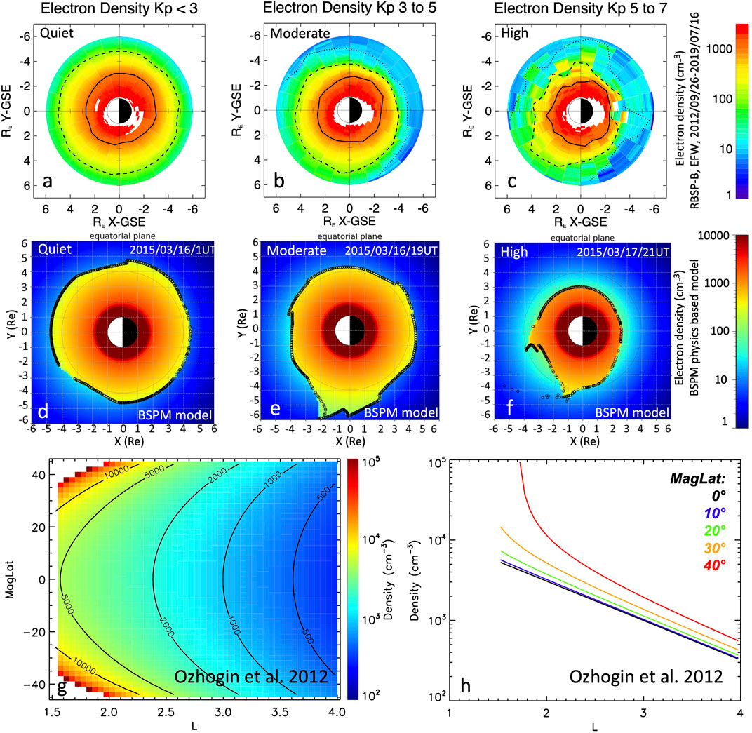
FIGURE 1. (A–C) Statistics of the electron plasma density (log₁₀ of the density in units cm^-3) from EFW on Van Allen Probes B during the whole mission (09/2012-07/2019) for 3 Kp bins of geomagnetic activity (Ripoll et al., 2022a). (D–E) The physics-based Belgian SWIFF Plasmasphere Model (BSPM) model of (color scale) the electron density and (black circles) the plasmapause during times of (D) quiet, (E) substorm, and (F) storm activity (Pierrard et al., 2021b). The empirical Ozhogin et al. (2012) density model derived from the IMAGE Radio Plasma Imager (RPI) measurement plotted (G) versus L-shell (L) and magnetic latitudes and (H) versus L-shell extracted at a few magnetic latitudes.

In this article, we review existing plasma density models, including ionospheric source models, empirical density models, physics-based and machine-learning density models. A great variety of conditions is considered such as the magnetic local time (MLT) variation, geomagnetic conditions, ionospheric source regions, radial and latitudinal dependence, and collisional vs. collisionless conditions. This review is framed in the context of radiation belt physics (see review in Ripoll et al., 2020a) and space weather codes. This implies the models are usually derived to be applied on the large spatial scales and large temporal conditions. Models that will be referred to and discussed are limited to those most commonly used for radiation belt simulations. We also focus on the more recent progress made during the last decade and to the promising models or data, such as those from the National Aeronautics and Space Administration’s (NASA) mission of the Van Allen Probes (Mauk et al., 2013). Models or data discussed in this review have gone through the calibration/correction analysis/process required to qualify the proper data to use (such as spacecraft potential correction, secondary electron effects, crosstalk effects correction in particle detectors, calibration corrections and modulation corrections on field detector antennae, etc.).

These models can be used to complement plasmaspheric densities inferred from satellite observations where or when data are lacking to fill data gaps, to be compared with these new data for evaluation, to be aggregated together or with observations to form more global models, or to analyze them for improving our understanding of the plasmasphere dynamics. Some of these models will serve as reference point or reference method from which we can improve and build a new generation of electron density models from the most recent observations, such as the NASA Van Allen Probes and the Japan Aerospace Exploration Agency (JAXA) Arase satellite missions (Miyoshi et al., 2018). The accuracy of the plasma density is essential for the computation of wave-particle interactions, which themselves determine the dynamics of the radiation belts.

2 The ionospheric source for the plasmasphere from the IRI model

The cold plasma in the plasmasphere has its origins in the ionosphere. Because the ionosphere is strongly driven by the Sun, the number density and temperature of the electrons, ions and neutrals in the ionosphere depend on solar activity, season, and local time, with a reset every day.

The earliest model of the topside ionosphere used only three bins in geomagnetic latitude and a linear dependence on F10.7 radio flux. In the 1990’s, a diffusive equilibrium model was used to compute the density in the topside ionosphere. The diffusive equilibrium model is a first-principles model that specifies the plasma density along a flux tube given boundary conditions at the footpoints (Angerami and Thomas, 1964). The boundary conditions include the number density and temperature of electrons, ions and neutrals. A diffusive equilibrium model is applicable at low altitudes where collisions are frequent, but may have limited utility at higher altitudes where the plasma is collisionless.

The main empirical model of the ionosphere, the International Reference Ionosphere (IRI), uses trigonometric functions to fit both temporal (local, seasonal, and annual) and spatial variations in measurements of electron density coming from worldwide network of ionosondes, powerful incoherent scatter radars, topside sounders, and in situ instruments flown on many satellites and rockets, with the coefficients depending on solar activity. IRI has several altitude regions of interest: the D, E, F1, and F2 regions, and the topside ionosphere, which extends from the F2 peak to the maximum altitude in the model, 2000 km in IRI-2012 (Bilitza et al., 2014) (see also Bilitza et al., 2017; Biliitza, 2018). The IRI model is driven by several solar and ionospheric indices including the sunspot number R, the solar radio flux at 10.7 cm wavelength F10.7 (Tapping, 2013), and the ionosonde-based ionospheric global (IG) index (Bilitza, 2018). Last version is IRI 2020 on irimodel.org.

More specifically, the transition from highly collisional to collisionless in the topside ionosphere makes it a particularly difficult region to model. In IRI-2007, the topside ionosphere model from NeQuick (Coïsson et al., 2006) was included as the default option. This model has been constructed from ISIS-2 topside sounder data orbiting at 1,400 km (see also Gulyaeva, 2012). Further extension to higher altitudes includes the work of Gulyaeva et al. (2002) who took available topside sounder profiles up to 3,500 km and built a connection of IRI to the bottom of the plasmasphere (IRI-PLAS) (see also Gulyaeva, 2011; Gulyaeva et al., 2011). Reinisch et al. (2007) also made an attempt to connect the IMAGE/RPI density data (see section 3.2) with IRI 2001 topside using the vary-Chap approach (see also discussion in Bilitza and Reinisch, 2008). This model was further improved in Nsumei et al. (2012).

3 Empirical models

3.1 Empirical plasma density models

Early efforts to model the plasmaspheric electron density included effects due to solar activity and season, with the first models providing the density using simple empirical relations depending on the McIlwain parameter L in Earth radii. Carpenter and Anderson (1992) derived a “reference profile” of the plasmaspheric electron density, valid for 2.25 < L < 8, to describe the saturated plasmasphere, $N (L) = 10^{(- 0.3145 L + 3.0943)}$ , with additional dependences to include perturbations due to season and phase of the solar cycle. This model uses the International Sun-Earth Explorer (ISEE) measurements and is limited to the local time interval of 0–15 MLT omitting plasma expansion on the dusk side, which these authors had aimed to treat separately (Carpenter and Anderson, 1992). Lyons and Thorne (1973) used a form $N (L) = 1000 {(4 / L)}^{4}$ , that was consistent with Carpenter et al. (1964), to derive electron lifetimes that yielded equilibrium flux profiles for L = [1,5] using a Fokker-Planck radial diffusion code, even though the density model was not valid below L = 2. Albert (1999) used an exponential, N(L) = 16400e^−0.875L, instead of a power law in L. Sheeley et al. (2001) reported N(L) = 1390 (3/L)^4.8 ± 440 (3/L)^3.6 in the plasmasphere for 3 ≤ L ≤ 7, where the authors show that the standard deviation captures differences between a newly filled and saturated plasmasphere. They did not find a magnetic local time (MLT) dependence for the plasmasphere, but did model the MLT-dependence of the plasma trough. A combination of Albert (1999) within the plasmasphere and Sheeley et al. (2001) within the plasma trough is used in the wave-particle interaction simulations of Ripoll et al. (2017) when satellite observations are lacking.

Gallagher et al. (2000) developed the Global Core Plasma Model (GCPM), a single unified model of the whole plasmasphere using an ‘amalgam’ of previously developed ‘region-specific’ models. GCPM addresses the density, temperature and composition of the plasmasphere, plasmapause, trough and polar cap. It depends on solar and geomagnetic indices, but is intended to be ‘representative’ of these conditions rather than used as a dynamic model. GCPM uses a modified version of the reference profile of Carpenter and Anderson (1992), N(L) = 10^−0.79L+5.3, added to the perturbations due to the solar cycle and season. It joins the topside ionosphere model of IRI to the equatorial plasma density model by first extrapolating the slope of the IRI model above the F2 peak using an exponential function and extrapolating the slope of the equatorial model downward in altitude with another exponential function, then blending the two functions with hyperbolic tangents. At higher latitudes, the shape of the exponential function is determined from IRI above the F2 peak, but the form is shifted by a constant so that the exponential decays to the equatorial value. The plasmapause location and width depend on local time. GCPM could be considered as the best compilation of all empirical density models. However, the GCPM model has not been directly coupled to radiation belt codes or wave particle interactions codes (to the knowledge of the authors) but it has been used for the validation of other plasma density models, themselves used in radiation belt codes (e.g., Ozhogin et al., 2012).

3.2 Latitudinal dependence

There have been recent efforts to model the variation of electron density with magnetic latitude. Denton et al. (2006) used satellite measurements from Polar and the Combined Release and Radiation Effects Satellite (CRRES) to model the latitudinal variations as a power law of the radial distance R to any point along the field line, $N (L, R) = N_{e q} {(L R_{E} / R)}^{α}$ , and fit $α$ as a function of L and equatorial density for L > 2. Denton et al. (2006) fit this model to IMAGE RPI data and found that it did not perform well at high magnetic latitudes. Reinisch et al. (2004) and Huang et al. (2004) found that the following form fits data from IMAGE RPI well:

N (L, λ) = N_{e q} (L) {[1 + γ λ / λ_{I N V}] [\cos ((π / 2) (α λ / λ_{I N V}))]}^{- β} (1)

where $λ$ is the magnetic latitude, $λ_{I N V}$ is the invariant magnetic latitude, and the fitting parameters are $α, β, γ .$ Ozhogin et al. (2012) built on the earlier work of Reinisch et al. (2004) and fixed the values of the fitting parameters to

α = 1.01 \pm 0.03, β = 0.75 \pm 0.08, γ = 0 a n d N_{e q} (L) = 10^{- (0.4903 \pm 0.0315) L + (4.4693 \pm 0.0921)} (2)

The Ozhogin et al. (2012) model is restricted to altitudes greater than 2000 km and L > 1.5, up to L = 4, and does not address dependence on MLT, season, solar activity, or differences in density between the Northern and Southern hemispheres. This model is plotted in Figures 1G, H to illustrate the increase of density with latitude. Models of Carpenter and Anderson (1992), Gallagher et al. (2000), Denton et al. (2006), Sheeley et al. (2001) and Ozhogin et al. (2012) are compared in Figure 8 of Ozhogin et al. (2012).

Empirical and first-principles models of the cold plasma density in the plasmasphere have been in development since the 1960’s, but there is just one model (Ozhogin et al., 2012) that is valid below L = 2 and includes latitudinal dependence. To our knowledge, there was no valid empirical model below L = 1.5, nor one that includes variations due to solar activity, season, local time, and hemispheric differences, in addition to $L, λ$ below L = 2. Recently, Hartley et al. (2023) combined Van Allen Probes data for latitudes below 20° with Arase data up to 40° for 1 < L ≤ 3 and derived a new electron density model with both a latitudinal and MLT dependence. Comparison with the L dependence of the Ozhogin model shows good agreement above L = 1.5. Below L = 1.5, a fitting form similar to the Ozhogin model is adopted with new parameters defined as $α = 1.03, β = 0.44$ . An MLT dependence of the plasma density was identified, which is consistent with the diurnal variation of ionosphere. This variation is strongest at low L, but persists out to L = 3. All empirical electron density models discussed in this article are listed and succinctly synthetized in Table 1.

TABLE 1

TABLE 1. Empirical electron density models discussed in this article.

3.3 Empirical plasmapause models

There exist a variety of empirical plasmapause models currently used in radiation belt simulations. They generally provide the radial distance of the plasmapause in the equatorial plane as a simple function of the geomagnetic activity level. Tu et al. (2009) used, for instance, the CRRES data driven model of O’Brien and Moldwin (2003), whereas Tu et al. (2013) implemented the Carpenter and Anderson (1992) plasmapause model (noted CA92). The CA92 plasmapause model is the most commonly used model to our knowledge. It has been largely used for radiation belt studies over the last 10 years (Subbotin and Shprits, 2009; Kim et al., 2011; Shprits et al., 2013; Ripoll et al., 2016; Ripoll et al., 2019; Wang and Shprits, 2019; Cervantes et al., 2020a; Cervantes et al., 2020b; Malaspina et al., 2020; Saikin et al., 2021).

Recently, Ripoll et al. (2022a) derived both a plasmapause and a 100 #/cc density level models based on the entire Van Allen Probes mission (2012-2019) from both the Electric and Magnetic Field Instrument Suite and Integrated Science (EMFISIS) suite’s (Kletzing et al., 2013) and the Electric Field and Waves (EFW) (Wygant et al., 2013) data. The cold plasma densities are either determined by the upper hybrid resonance (UHR) method from EMFISIS measurements (Kurth et al., 2015) or by using the spacecraft floating potential (Escoubet et al., 2007; Torkar et al., 2016; Torkar et al., 2019) measured by the Electric Field and Waves (EFW) instrument (Wygant et al., 2013).

About the accuracy of these density measurements, we note the densities derived along with the corresponding spacecraft potentials are fit to a function with a non-linear least squares fit. The resulting fits typically have a Pearson (R²) coefficient in the range of ∼0.75–0.95 and an average percent error between the selected fit derived densities and the densities used to perform the fit of ∼15%. Experiments with individual orbits show that fits of the functional form can capture the density voltage relation over a range of densities from ∼few cm^-3 up to 3,000 cm^-3 with the lower densities still agreeing with the EMFISIS UHR densities to within 10%. However, using the same fit for a longer period (larger than an orbit) the EFW and EMFISIS densities may diverge by over factor of two at densities <10 cm^-3. The reason for this is the variability of the plasma environment outside the plasmasphere. For periods during which the upper hybrid resonance line is clearly resolved in the High Frequency Receiver (HFR) spectral data, the EMFISIS density product is generally more accurate than the EFW. However, during times in which there are high levels of wave activity that make identification of the upper hybrid line difficult or impossible, resulting in increased uncertainty in the EMFISIS densities, the EFW density fits still return densities by applying the relevant fit equation to the spacecraft potential. Regarding the semi-automated process for determining the EMFISIS density from the UHR (Kurth et al., 2015), there is a 8.7% mean percentage difference between the manual process and the semiautomatic process, which is less than the ∼10% resolution available for an individual measurement. This difference is visible in Figure A2 of Goldstein et al. (2014a), where the average difference is often low (∼7%), is less than 20% in general, but can be up to 100% for a very small number of data points. Another main source of error is the spectral resolution, due to the upper hybrid resonance that can only be defined at specific values dictated by the binned frequency spectrum. This translates to a density resolution of Δne/ne of about 10%. The uncertainty increases when the spectra become difficult to interpret, as discussed in Goldstein et al. (2014a). In most instances, the spectral resolution uncertainty is estimated to be between 10% and 20% (Hartley et al., 2016). The EMFISIS and EFW densities from ∼10 cm^-3 to 3,000 cm^-3 are statistically compared in Jahn et al. (2020), who found that the EFW values predominantly fall in a range of 50%–200% of their corresponding EMFISIS measured value (e.g., 0.5 to 2 times the actual value), while most of the EFW to EMFISIS points used for comparison are ∼100% (e.g., n_EFW ∼ n_EMFISIS). Further comparisons of the 100 #/cc level are carried out in Ripoll et al. (2022a) in which Figures 1K, L confirm the good agreement between both methods, with the bulk of normalized differences below ±20%.

A comparison of the CA92 plasmapause model with Van Allen Probes measurements is performed in Ripoll et al. (2022a). These authors first recover the CA92 model using EMFISIS data and a gradient method to localize the plasmapause, showing the practical reliability of the CA92 model. However, direct comparisons of the 100 cm^-3 level deduced from Van Allen Probes EFW measurements and the CA92 model show the dense plasmasphere expands farther out than predicted by the CA92 model. Departure of the CA92 model from the 100 cm^-3 EFW data increases as the maximum value of the Kp index over the last 24 h (Kp) increases and L-shell decreases, and storm-induced erosions are less deep than predicted by the CA92 model (Ripoll et al., 2022a).

The model of O’Brien and Moldwin (2003) based on CRRES data is the first to show the MLT dependence as well as the relevance of parametrizing the plasmapause model with various indices, such as Kp, AE, and Dst (see also Moldwin et al. (2002)). Carpenter et al. (2000) states the experimental error in the CRRES density is associated with measuring the UHR or plasma frequencies on the SFR records. They estimated to be +/− 6% in spectral resolution (Δf/f), which corresponds to +/− 12% in density. Kwon et al. (2015) derived the median/mean plasmapause locations from the electron density inferred from the Time History of Events and Macroscale Interactions during Substorms (THEMIS) spacecraft potential under steady quiet conditions (Kp ≤ 1). The comparison of their plasmapause model with the estimated Lpp from models such as GCPM (Gallagher et al., 2000), Moldwin et al. (2002), and O’Brien and Moldwin (2003) with Kp = 1 shows the plasmapause is farther extended ∼1–2 L from the Earth (i.e., GCPM and CRESS based-models models underestimate the extend of the plasmapause). Ripoll et al. (2022a) show the underestimation of the plasmapause position is caused by the gradient method that fails identifying gradients particularly during quiet times and on the dusk.

Other plasmapause models include Bandić et al. (2016) based on CRRES data, Cho et al. (2015), Liu and Liu (2014) and Liu et al. (2015) based on THEMIS data, and Larsen et al. (2007) based on IMAGE data. Verbanac et al. (2015) plasmapause model is based on CLUSTER data and analytical relationships obtained from geomagnetic and solar wind observations. Bandic et al. (2017) derived a plasmapause model from a large dataset including multiple sources. A comparison of these models is provided in Pierrard et al. (2021c) showing a great variability of mean plasmapause empirical models (see also Guo et al., 2021). All empirical plasmapause models discussed in this article are listed and succinctly synthetized in Table 2 (see also Table 1 in He et al. (2017) listing the model dependences).

TABLE 2

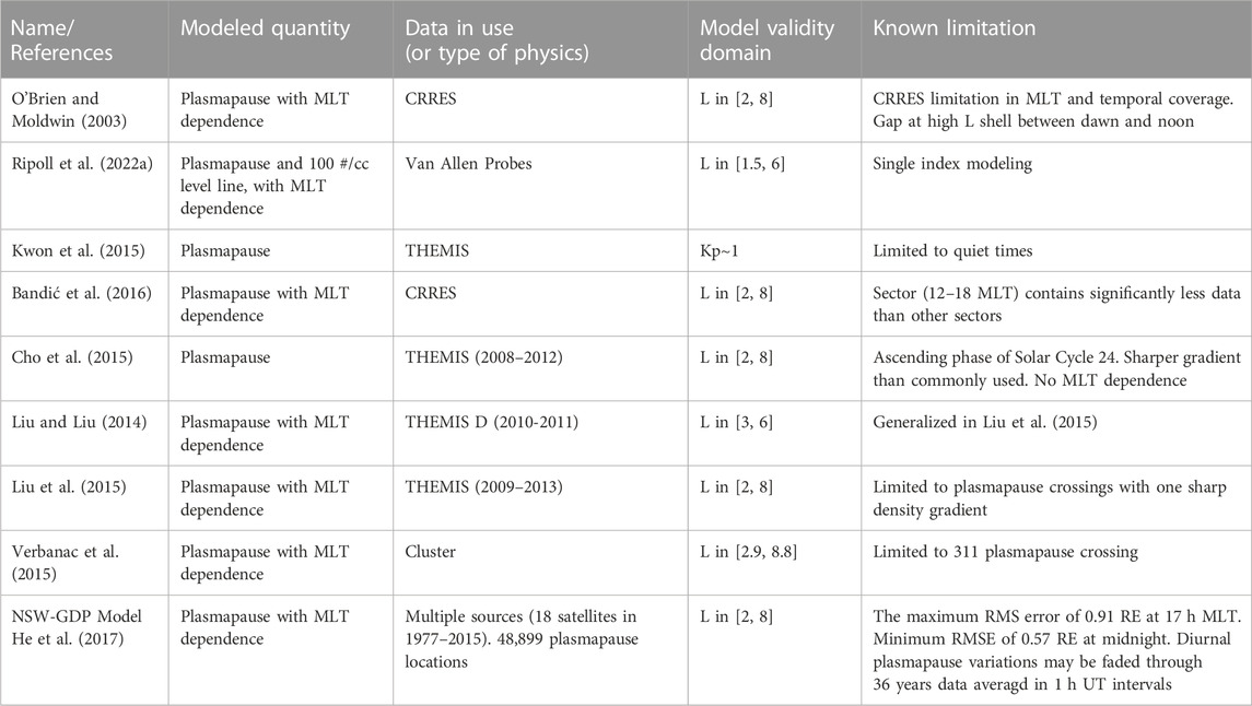
TABLE 2. Empirical plasmapause models discussed in this article.

The large variability of the measurements underlying the mean empirical plasmapause models (more generally mean plasma density empirical models) is one major limitation of this type of models that calls for the use of either physic-based models or machine learning technics.

4 Physic-based models of the plasmasphere

4.1 Ionosphere-plasmasphere models

The 3D global ionosphere/plasmasphere fluid model SAMI3 (Huba and Krall, 2013; Krall and Huba, 2013) of the Naval Research Laboratory (NRL) solves the continuity and momentum fluid equations for seven ion species (H⁺, He⁺, N⁺, O⁺, N⁺₂, NO⁺ and O⁺₂) and includes the thermospheric wind-driven dynamo electric field. It is based on SAMI2 (Huba et al., 2000). SAMI3 uses the partial donor cell method (Hain, 1987; Huba, 2003) and a newly implemented 4-order flux-corrected transport scheme for ExB transport perpendicular to the magnetic field (Huba and Liu, 2020). The temperature equation is solved for three atomic ion species and electrons. The model has a co-rotation potential, a neutral wind dynamo potential (with winds from HWM93 (Hedin, 1987)), and a time-dependent Volland-Stern-Maynard-Chen potential. In Huba and Krall (2013), SAMI3 density results are compared at the equator for 4 MLT sectors with the quiet time empirical electron density of Berube et al. (2005) defined as n_eq = 10^0.51L+4.56 for L in 2–5 from IMAGE RPI data between May 2000 and May 2001. They find the SAMI3 electron density is lower by a factor 2 attributed to a lower F10.7 index used in the simulation.

The SAMI3 model has been recently modified to support the NASA ICON mission and provide ionosphere and thermosphere properties during this mission (Huba et al., 2017). SAMI3 recently integrated an improved model of counterstreaming H⁺ outflows from the two hemispheres during storm using a two fluid species for H+ (Krall and Huba, 2019) in order to avoid non-physical high-altitude ‘top-down refilling’ density peaks (Krall and Huba, 2021). SAMI3 is currently used to try to reproduce the formation of density ducts in the plasmasphere (e.g., Jacobson and Erickson, 1993; Loi et al., 2015) caused by the thermosphere composition and winds on plasmaspheric refilling outflows (Krall et al., 2018) as observed from the Murchison Widefield Array (MWA) interferometric radio telescope in Australia (Helmboldt and Hurley-Walker, 2020). SAMI3 recently coupled to the atmosphere/thermosphere code WACCM-X (Whole Atmosphere Community Climate Model with thermosphere and ionosphere extension) provided the first high-resolution global simulation using realistic thermospheric conditions of the formation and penetration of plasma bubbles into the topside F layer (Huba and Liu, 2020). These structures will further propagate to higher altitudes and introduce longitudinal and seasonal dependence structures into the plasmasphere. Further coupling of SAMI3 and applications are discussed in Huba (2023).

The Ionosphere-Plasmasphere-Electrodynamics (IPE) model is derived in Maruyama et al. (2016) to investigate the connection between terrestrial and space weather (e.g., Fuller-Rowell et al., 2008). IPE provides 3D thermal plasma densities for nine ion species, electron and ion temperatures, and parallel and perpendicular velocities of the ionosphere and plasmasphere. The parallel plasma transport is based on the Field Line Interhemispheric Plasma (FLIP) Model (Richards et al., 2010). There is a detailed model of the Earth’s magnetic field using Apex coordinates (Richmond, 1995) and the International Geomagnetic Reference Field IGRF (as in SAMI3). The transport is computed with the same solver all the way from the equator to the pole on a global static grid with a semi-Lagrangian scheme that allows for the global plasma transport perpendicular to magnetic field lines. There is a self-consistent photoelectron calculation enabling more accurate studies of the longitudinal/UT dependence of the ionospheric mass loading process. IPE is generally defined from 90 km to approximately 10,000 km. The spatial resolution of the radial direction in the plasmasphere varies from 0.05 R_E (L = 1.5) to 0.46 R_E (L = 5). IPE has used to reproduce the Weddle Sea Anomaly (Sun et al., 2015) and for studying extreme plasmaspheric erosion as low as L∼1.7 (Obana et al., 2019). Current applications of IPE include plasmaspheric drainage plumes, ionospheric storm enhanced density (SED) plumes, plasmaspheric refilling, and plasmaspheric composition. The Whole Atmosphere Model (WAM)(e.g., Akmaev and Juang, 2008) has been coupled with IPE (WAM-IPE) and provides today space weather forecast 24/7 at NOAA SWPC (https://www.swpc.noaa.gov/products/wam-ipe). WAM-IPE has recently be used to simulate ESF irregularities (Hysell et al., 2022).

The IRAP Plasmasphere Ionosphere Model (IPIM) uses a 16-moment approach for strong temperature anisotropy at high altitude and for accurately modeling the transition between collision dominated at low altitude and collisionless media at high altitude (Marchaudon and Blelly, 2015). IPIM solves the interhemispheric hydrodynamics convection and corotation of six ions and thermal electrons along flux tubes at different distances from Earth. IPIM has a kinetic model for suprathermal electrons and solves for the chemical reactions in the ionosphere. IPIM has been used to simulate the depletion of the ionospheric F₂ layer by a high-speed stream for short-term behavior on the scale of a few hours Simulations were found to be consistent with EISCAT radar and the ionosonde measurements (Marchaudon et al., 2018). For the long-term evolution of the plasmasphere-ionosphere system and during quiet conditions, IPIM simulations indicate that the plasmasphere in not stable in MLT and that no real dynamic equilibrium can be reached (Marchaudon and Blelly, 2020).

4.2 Plasmasphere models

Different plasmasphere models combining semi-empirical relations and physics-based backgrounds have been developed to reproduce the inner magnetosphere, the plasmapause, and even the plasma trough above the plasmasphere limit (see Pierrard et al., 2009 for a review of the plasmasphere models before 2009).

Pierrard and Stegen (2008) have developed the Belgian SWIFF Plasmasphere Model (BSPM), a 3D dynamic kinetic model of the plasmasphere. The BSPM model is based on physical mechanisms, including the interchange instability for the formation of the plasmapause (Pierrard and Lemaire, 2004), and provides the density and the temperature of the electrons, protons and other ions, both inside and outside the plasmasphere in the plasma trough. It has been coupled to the ionosphere (Pierrard and Voiculescu, 2011) using the IRI model as a boundary condition and is continuously improved by including other physical processes like plasmapause thickness and plasmaspheric wind (Pierrard et al., 2021b). The input of the model is the date that determines the geomagnetic indices Kp and Dst. The plasmapause position does strongly correlate with the Bartels geomagnetic index, Kp index, which is retained as the main parameter used in the model to determine the plasmapause position. These indices may be predicted values when forecasting is required, or observed values when past events are simulated. They determine also the convection electric field. As BSPM uses the IRI model, it also depends on IRI parameters listed in Section 2. The BSPM model includes plasmapause erosion during geomagnetic storms as well as refilling, and is able to reproduce the plumes generated during storms and other structures like shoulders. It uses the kinetic approach that allows for the inclusion of non-Maxwellian distributions (Pierrard and Lemaire, 2001). The last version of the BSPM model is shown in Figures 1D–F for quiet, substorm, and storm activity. On 16 March 2015 1H (UT) with a quiet period with Kp∼2 (and almost constant during several hours), the plasmasphere is quite extended and almost circular (to compare with Figure 1A). A few hours later after a substorm injection on 16 March 2015 19 h (UT) with Kp∼4, there is formation of a plume in the dusk sector rotating with the Earth (to compare with Figure 1B). On 17 March 2015 21 h (UT) during an intense storm with Kp = 8^-, the model shows a strong erosion of the plasmasphere and formation of a long plume rotating with Earth (to relate with the statistics of Figure 1C).

The kinetic approach based on particle-in-cell simulations has also been combined with the fluid approach in Wang et al. (2015) to develop a dynamic fluid-kinetic model for plasma transport within the plasmasphere. A semi-kinetic model of plasmasphere refilling following geomagnetic storms has also been recently developed by Chatterjee and Schunk (2020b) and compared with hydrodynamic models to explore their differences. In hydrodynamic plasmasphere models, the non-linear inertial terms in the plasma transport equations are retained (Chatterjee, 2018; Chatterjee and Schunk, 2019; Chatterjee and Schunk, 2020a; Chatterjee and Schunk, 2020b). Limitations of such models are generally related to the difficulty to reproduce the mechanisms implicated in the formation of the plasmapause and the refilling process that is a key physics-based problem to solve to obtain a fully coupled plasmasphere-ionosphere model.

A two-dimensional physics-based plasmasphere model called Cold Plasma (CPL) (Jordanova et al., 2006; Jordanova et al., 2014) is used in a ring current-atmosphere interactions model of the source and loss processes of refilling and erosion driven by empirical inputs to simulate equatorial plasmaspheric electron densities. The performance of CPL has been evaluated against in situ measurements by the Van Allen Probes (Radiation Belt Storm Probes) for two events (De Pascuale et al., 2018). This study finds that severe erosion is best captured by an effective Kp-index for scaling the inner-magnetospheric potential governing E x B flows while refilling subsequent to moderate activity requires a solar wind parameterization of the quiet time background after the onset of a geomagnetic storm. Empirical models driving plasmasphere dynamics can be improved by capturing localized enhancements in electric field measurements and asymmetric profiles in electron density observations. More specific simulations were dedicated to comparisons with Van Allen Probes plasmapause observations (Goldstein et al., 2014a; Goldstein et al., 2016).

4.3 Plasmapause models

Physics-based models also provide the plasmapause location (e.g., Pierrard et al. (2021b)), with some models integrating Van Allen Probes measurements and plasma trough densities (e.g., Botek et al., 2021). Goldstein et al. (2003), Goldstein et al. (2005) developed a plasmapause test particle (PTP) dynamic model that represents the plasmaspheric boundary as an ensemble of E × B-drifting particles. The PTP model uses an electric field which is driven by the solar wind E field and Kp. The evolution of the plasmapause is modeled by the changing shape of the curve defined by the aggregate of the test particles evolving in a time-varying convection E-field. PTP simulation for the moderately disturbed interval 18–20 January 2000 shows a narrow drainage plume followed by significant plasmaspheric erosion, forming a second plume that coexists with the residue of the first plume (Goldstein et al., 2014b). Observations from three of the Los Alamos National Laboratory geostationary satellites are globally consistent with this PTP simulation in terms of the durations of plume sector transits while the MLT widths and timings of the simulated plumes do not precisely agree (Goldstein et al., 2014b). Goldstein et al. (2019) further generated a plasmapause statistical model from the simulations of 60 storms with Dst,_PEAK ≤ −60nT based on Van Allen probes data yielding over 7 million model plasmapause locations. The epoch-binned PTP simulation results are combined in order to create an analytical plasmapause model for moderate storms (−120nT ≤ Dst,_PEAK ≤ −60nT) and strong storms (Dst,_PEAK ≤ −120nT) that explicitly includes plumes. This model depends on the duskside plasmapause radius and two fitted coefficients, all three depend on epoch time (from −24 h to 36 h).

4.4 Global geospace model

A new promising approach is to couple a global geospace model of the magnetosphere with a physics-based density model. Figure 2 provides an example of the global geospace model, GAMERA (Zhang et al., 2017; Sorathia et al., 2020; Sorathia et al., 2021) coupled to RCM (Toffoletto et al., 2003). With a two-way coupling, these models are subparts of the Multiscale Atmosphere-Geospace Environment (MAGE) (e.g., Chen et al., 2021; Pham et al., 2021; Lin et al., 2022). The details of GAMERA’s core MHD numerics and its verification are presented in Zhang et al. (2019). GAMERA uses high-order spatial reconstruction for the preservation of sharp structures. For typical MHD problems, Zhang et al. (2019) showed lower-order reconstruction (e.g., Second-order) requires four to eight times finer grid resolution (corresponding to a 250-4,000 factor increase of the cost resolution in 3D) as the higher-order (seventh- or eighth-order) reconstruction to reach the same accuracy. In addition to coupling the global MHD model to the inner magnetosphere model via ring current pressure ingestion (e.g., Pembroke et al., 2012), here the RCM is additionally evolving a cold fluid to model the evolution of the plasmaspheric density. In this coupling, the plasmasphere density is initialized using an empirical model (Gallagher et al., 2000) and refilling rate (Denton et al., 2012), and evolved using the same dynamically-calculated electrostatic potential as in the MHD simulation (e.g., Merkin and Lyon, 2010). Note that RCM can further be coupled with SAMI3 as done by Huba et al. (2017b) to study the ionosphere-plasmasphere system response to the 17 March 2015 geomagnetic storm. The coupling occurs through the electrostatic potential equation (Huba et al., 2005; Huba and Sazykin, 2014) in which the conductance is defined by the sum of the conductance associated with solar activity computed by SAMI3 and the auroral enhanced conductance provided by RCM.

FIGURE 2

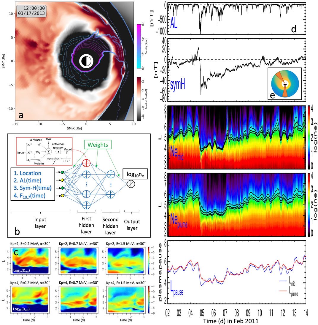
FIGURE 2. (A) Coupled GAMERA global geospace model and RCM simulation depicting localized nightside dipolarizations and dayside plasmaspheric plume. Shown is the non-dipolar component of the northward magnetic field (left color bar) and contours of constant density (right color bar) in the equatorial plane (Sorathia et al., 2018). (B) The neural network architecture of DEN2D in Chu et al. (2017a). (C) Predictions of diffusion coefficients for variable density and wave properties from the neural network model of Ripoll et al. (2022b) during (top) quiet (Kp = 2) and (bottom) moderate (Kp = 4) activity. A Kp-based model of plasma density and wave properties would find constant values in time. (D) Density and plasmapause location predicted by the DEN2D neural network at midnight (noted mid) and in the plume (noted plume) based on the AL and Sym-H indices in February 2011 during a refilling event showing dynamic rates of refilling (Chu et al., 2017b). (E) Equatorial density predicted by DEN2D and MLT sectors shown in (D).

Figure 2A depicts localized dipolarizations on the nightside and the formation of a dayside plasmaspheric plume during the 17 March 2013 geomagnetic storm (Sorathia et al., 2018). There is a complex interacting mesoscale process with nightside flows, boundary Kelvin-Helmholtz on the dayside and flanks, and rolling dense plasmaspheric plume and structures. The plume is shown at 12 UT, i.e., 6 h after the CME impacted the Earth, with a typical expansion in the dusk-day sector that reaches L∼6 and has started to roll around Earth.

The Kelvin-Helmoltz instability we see forming on the magnetopause and rolling side way of the magnetosphere (Merkin et al., 2013) may contribute to transfer shear and turbulence to the plume as it expands and removes pockets of dense plume plasma. In this way, the plume may potentially inherit a complex shape that is here captured by the global MHD model. The dense plasmasphere has a circular aspect for levels above 1,000 #/cc and there are structured plasma pockets of low density from 1-10 #/cc on the nightside beyond the main plasmapause gradient at L∼3. On the night side, the magnetic field (and similarly the electric field) has a fine scale structure (with finger-like regions of higher field value) that reach the L∼6 region and imprint a fluctuating profile to the dense pockets down to the plasmapause layer. As simulation resolution increases, some aspects of these structures become finer and more torturous. However, understanding the full cascade of energies down to the smallest scales requires global kinetic modeling.

These kinds of mesoscale structures play a critical role in shaping both the global-scale and micro-scale processes of the magnetosphere. Localized injections are believed to be an important part of the transport of magnetic flux and energetic particles into the inner magnetosphere (e.g., Gkioulidou et al., 2014; Merkin et al., 2019), thus building the large-scale ring current and affecting global dipolarization of the inner magnetosphere, as well as resulting in density enhancements at the dayside magnetopause that will alter local reconnection rates (e.g., Zhang et al., 2017) with potentially global consequences. Additionally, these mesoscale processes shape the different wave populations of the inner magnetosphere: anisotropic ion injections provide free energy for the ElectroMagnetic Ion Cyclotron (EMIC) wave population and the evolving plasmapause boundary correlates with the relative distribution of hiss and chorus waves, with important consequence on flux enhancements of energetic trapped particles in the radiation belts. Physics-based models discussed in this article are listed and succinctly synthetized in Table 3.

TABLE 3

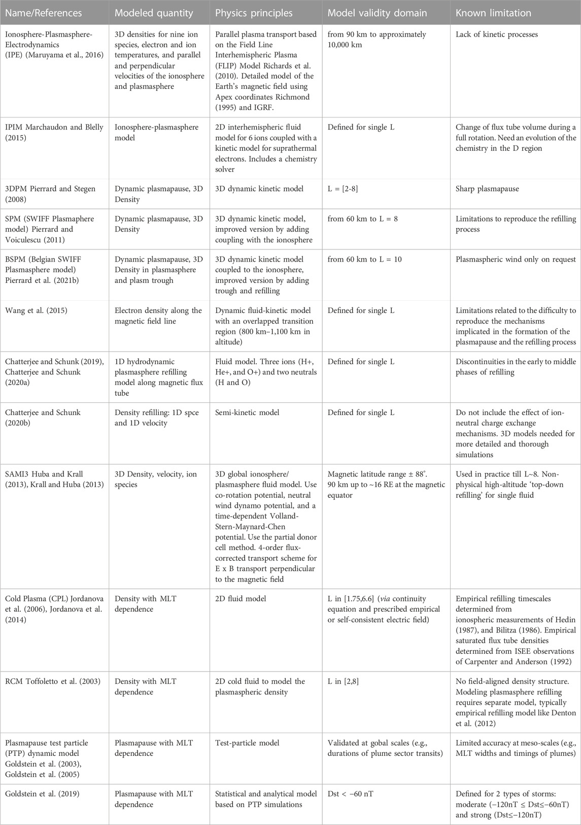
TABLE 3. First-principles physics models discussed in this article.

5 Machine learning models

Machine learning (ML) techniques have advanced significantly over the past decade, especially during the past few years, mainly due to three factors: enormously increased volumes of data, significantly improved algorithms, and substantially more-powerful computation hardware (especially Graphics Processing Unit (GPU) computation that can accelerate the training by a factor of ∼100) (Goodfellow et al., 2016). Although the applications of ML techniques are not entirely new in space physics, the unique combinations of the three aforementioned factors are leading to a new era where proper ML techniques could significantly enhance scientific progress, especially in understanding the non-linear nature of many physical processes. The combination of density data and models through machine learning techniques is one of the future and promising paths.

Taking advantage of the improvements in ML techniques and the extensive spatiotemporal coverage of NASA satellites, a series of ML-based models have been developed to study the cold plasma density for two purposes: 1) providing time- and history-dependent global distributions of total electron density in the Earth’s magnetosphere, and 2) automatic detection of upper-hybrid-resonance frequency to calculate the total electron density.

A ML-based method was first proposed to reconstruct the global and time-varying distributions of any physical quantity Q that is sparsely sampled at various locations within the magnetosphere at any time (Bortnik et al., 2016). A feedforward neural network model was developed using point measurements of total electron density (i.e., cold plasma density) inferred from THEMIS spacecraft potential as an illustrative example. The model additionally takes the time series of the sym-H index as input and reconstructs global distributions of electron density at any time. Later, an optimized model of the electron density (DEN2D) near the equatorial plane was developed using THEMIS data (Chu et al., 2017a). The optimal input parameters of the DEN2D model are determined to be sym-H, AL, and F10.7 indices based on the neural network and neuron illustrated in Figure 2B. Time series of these indices are used as input so that the DEN2D model is both time- and history-dependent (i.e., dependent on a time sequence). The DEN2D model succeeds in reconstructing various plasmaspheric features during a geomagnetic storm, such as quiet time plasmasphere, erosion, and refilling of the plasmasphere and plume formation. Figures 2D, E shows the DEN2D density prediction extracted at both midnight and in the afternoon/day sector during plume expansion in February 2011. Analysis of these results demonstrated that refilling rates are dynamically changing (Chu et al., 2017b). The uncertainty of the DEN2D model can be estimated using a probabilistic model (Camporeale et al., 2019). Using global density profiles from the DEN2D model, it is shown that plasmaspheric hiss wave power is better parameterizing by plasma density rather than L shell, which should be adopted in current empirical models (Malaspina et al., 2018). A three-dimensional model of the electron density (DEN3D) was further developed using point measurements of the cold plasma density inferred from the upper hybrid resonance obtained from equatorial (ISEE and CRRES) and polar-orbiting satellites (POLAR and IMAGE). It has been verified using the additional measurements of density along the field line provided by IMAGE RPI (Chu et al., 2017b). The DEN2D and DEN3D models are shown to represent a large fraction of the observed variability in plasma density, with correlation coefficients on the order of 0.95, and a root-mean-square (rms) uncertainty about a factor of 2. There is room for improvement, since the model uncertainty is larger than the relative error of the underlying density measurements that are typically close to, or less than, 20% (Reinisch et al., 2004). For example, the confined density enhancements or depletions (ducts) may contribute to the model uncertainty since these localized structures may not be accurately predicted using geomagnetic indices. The DEN2D and DEN3D models can reconstruct the electron density with much smaller bias and error compared to previous empirical models (e.g., Global core plasma model (Gallagher et al., 2000; Sheeley et al., 2001; Denton et al., 2004; Denton et al., 2006), and the model of Ozhogin et al. (2012)), although the model of Ozhogin et al. (2012) has competitive performance inside the plasmasphere at the lowest L shells. DEN3D’s predictive ability provides unprecedented opportunities to gain insight into the 3-D behavior of plasmaspheric features (e.g., plasmaspheric erosion and refilling, as well as plume formation). Using a recurrent neural network, Huang et al. (2022) shows that the model could predict the formation and evolution of stable and evident plume configuration.

An electron density model of equatorial electron densities (PINE) was developed using Van Allen Probes measurements (Zhelavskaya et al., 2017). The PINE model also successfully reproduced erosion of the plasmasphere on the nightside and plume formation and evolution. However, ML-based models in space physics usually suffer from the problem of imbalanced dataset, i.e., many days of quiet conditions and a few days of storms (Camporeale, 2019). To overcome this difficulty, a coupled model was developed by using data assimilation, which is a weighted average of the neural-network-based PINE model for quiet times and a physics-based plasmaspheric model for active times, to provide the plasma density during both quiet times and geomagnetic storms (Zhelavskaya et al., 2021). In addition to modeling electron density, a neural-network-based model was developed to reconstruct the time-varying plasmapause location near the equatorial plane, which outperformed previous empirical models within its database (Guo et al., 2021).

The application of ML density models in Fokker-Planck diffusion model has been performed in Ma et al. (2018) and Bortnik et al. (2018). Neural networks (and other ML techniques) can also be used to perform assimilation and interpolation/extrapolation of large datasets. Diffusion coefficients computed from variable density and wave properties are directly embedded in a machine learning model in Kluth et al. (2022). Predictions of this model for 3 days of quiet (Kp = 2) and moderate (Kp = 4) times following the storm are shown in Figure 2C (Ripoll et al., 2022b). Temporal variations are related to the simultaneous change of density and wave properties, calling for future models that will couple density and wave properties together. A Kp-based model of density and wave properties, as commonly used nowadays, would find constant values of the diffusion coefficients in time at fixed L-shell in Figure 2C while the ML model shows multiple variations with time.

The ML techniques can also be applied to labor-intensive tasks. For example, the electron densities can be inferred from plasma wave spectra, which can be both time-consuming and challenging (e.g., Kurth et al., 2015). A neural-network-based upper hybrid resonance (UHR) determination algorithm (NURD) was developed to automatically determine the electron density from plasma wave measurements using Van Allen Probes data (Zhelavskaya et al., 2016, 2018; 2020). NURD is applied to Van Allen Probes EMFISIS data in Allison et al. (2021) to show that the plasma density has a controlling effect over acceleration of radiation belt electrons to ultra-relativistic energies. ML-based methods for automatically determining the UHR frequency have also been applied to the Arase satellite using convolutional neural network (Hasegawa et al., 2019; Matsuda et al., 2020) and the CLUSTER mission using several automated pipelines based on neural network methods (Gilet et al., 2021). Machine models of the electron density discussed in this article are listed and succinctly synthetized in Table 4.

TABLE 4

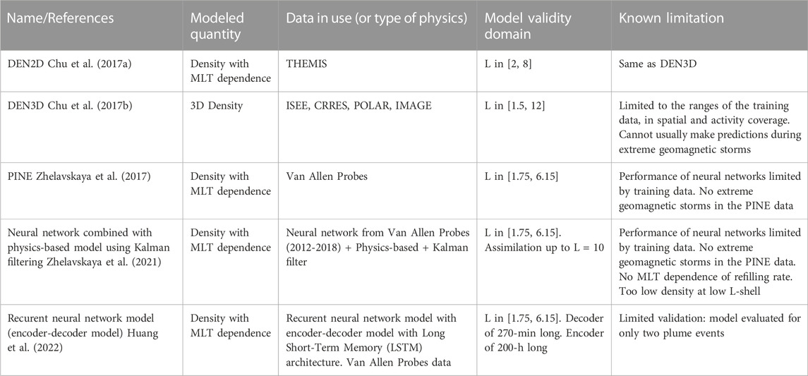
TABLE 4. Machine learning models of the electron density discussed in this article.

6 Conclusion and perspectives

This review article strictly focuses on existing plasma density models, with an emphasis on those most commonly used (or most recent or promising) in radiation belt physics or space weather codes. Plasma density models describe the state of the plasmasphere in radiation belt simulations and are at the heart of the coupling between the ionosphere, which provides the plasma source, and the magnetosphere, wherein the intensity and variability of wave-particle interactions are conditioned by the plasma density (see Thaller et al., 2022 and references therein). All models discussed in this review article are listed in Tables 1, 2, 3, 4 with their main properties listed.

This review shows that most of the current empirical density or plasmapause models in use for the last decade are relatively simple in their geomagnetic activity dependence, often including a dependence on a single geomagnetic index, e.g., Kp (Carpenter and Anderson (1992)), and not including a magnetic local time dependence. Some of these models are incomplete, limited by either short temporal coverage, such as those extracted from CRRES measurements (e.g., O’brien and Moldwin, 2003), or omitting magnetic local time sectors (Carpenter and Anderson (1992)) or geomagnetic activity (Ozhogin et al. (2012). The variability of the electron plasma density is also very large when sorted with a single index, even if retaining magnetic local time dependence (see Figure 3 of Ripoll et al., 2022a). The spatial and temporal variations in plasma density depend on multiple parameters, such as the refilling rate, which is itself dependent on UV irradiance, the state of the thermosphere (neutral winds, composition, etc.), and the time history and level of convective processes due to geomagnetic activity, the coupling between the magnetosphere and ionosphere, particle precipitation, and other processes. For instance, the standard deviation of the 100 #/cc density level (assimilable to the plasmapause) varies from ∼±0.5L for quiet times (Kp < 2, AE<300, Dst > −50) up to ∼±1L for active times (Ripoll et al., 2022a). This variability can be explained from the multiple factors that influence the plasmaspheric density. For instance, Denton et al. (2006) retained in their plasma mass density model, the F10.7 EUV index, magnetic local time, the solar wind dynamic pressure Pdyn, the phase of the year, and the solar wind B_Z in GSM coordinates (parameters listed in order of decreasing importance). Chu et al. (2017a) found the optimal input parameters of the neural network DEN2D model are the sym-H, AL, and F10.7 indices. This highlights that new models should keep the main parameter dependences, including ionospheric and geomagnetic variability, and the MLT dependence.

Density variations are well observed between L∼1.5 and L∼6 at each pass of the Van Allen Probes (see Figure 2F in Ripoll et al., 2017), thus directly influencing the diffusion coefficients describing wave particle interactions in the radiation belts. Diffusion coefficients vary linearly with the electron plasma frequency, f_pe(N), however changes in density further correlate with changes in the power of plasmaspheric hiss waves, which typically reside within the plasmasphere. Wave power is found to increase as density increases (Malaspina et al., 2016; Malaspina et al., 2018; Thomas et al., 2021). As a result, the simultaneous change in both density and hiss power leads to strong and complex variations of the diffusion coefficients (see Figure 5 in Ripoll et al., 2017). For instance, substorm activity causes short duration (within ± 4 h) reductions in density, and therefore a lowering of the amplitude of the whistler-mode waves within the plasmasphere. Variation in these parameters causes opposite effects in terms of pitch angle diffusion and, eventually, an overall decrease of pitch-angle diffusion during the main substorm activity (Ripoll et al., 2020b). Therefore, an accurate description of the plasma density, and its variation with geomagnetic activity, directly impacts the accuracy of modeling wave particle interactions.

The large number of parameters and mutually interdependent processes operating over different spatial and temporal scales, as just described, require models that include detailed physics or use machine learning methods in order to accurately capture or model these diverse plasma density features. Physics-based models have progressed well in the last decade, for instance, from 2D to 3D (e.g., Huba and Krall, 2013; Pierrard et al., 2021b) or by introducing new physical models or couplings, for instance, with detailed atmospheric sources (e.g., Huba and Liu, 2020). Physics-based models intrinsically simulate the geomagnetic activity and can retain various geomagnetic indices, whether these codes are limited to the atmosphere/ionosphere/plasmasphere system or are more global MHD codes, such as the MAGE-GAMERA project (e.g., Sorathia et al., 2021). It is only nowadays that physics-based models have started to be coupled with radiation belt codes (e.g., Dahmen et al., 2022), due to the overall complexity and multiplicity of the physical processes modeled in radiation belt codes (Ripoll et al., 2020a). An undeniable strength of physics-based models is that they can mitigate the inherent limitations of sparse spatial coverage of the data, in particular for active times (e.g., Zhelavskaya et al., 2021). Machine learning models also account intrinsically for multiple dependences (e.g., Chu et al., 2017a; Zhelavskaya et al., 2021), and are undoubtedly a promising approach to combine multiple satellite observations and produce the next-generation of global empirical plasma density models. A neural network-based density model has recently served to show that the plasma density has a controlling effect over acceleration of radiation belt electrons to ultra-relativistic energies (Allison et al., 2021). Contrary to empirical fits that do not allow trustable extrapolation, machine learning techniques, such as neural networks, are extremely promising in terms of predictive capability, which is a keystone for space weather codes. Progress in neural network technics are also expected in the coming years. For instance, the use of the recent physics-informed neural networks (e.g., Raissi et al., 2019), in which the neural network is constrained to respect any given physical law described by general non-linear partial differential equations, could be an hybrid way between physics-based models and machine learning technics, possibly well applying to plasma density modeling. Finally, the close relationship between plasmaspheric waves and plasmaspheric density also highlights the need for more coupling between them, whether that coupling is done when generating physical models or embedded within macroscopic quantities such as diffusion coefficients (e.g., Kluth et al., 2022).

In any case, all models eventually aim to capture the effect caused by magnetic local time variations of the plasma density for various geomagnetic conditions. There is an undeniable need of new measurements to support model development and validation. However, most measurements of the electron density used to build and/or validate these models, are often single observation per time at a single location in space, leading to a reliance on statistics to capture the magnetic local time resolution. This reliance on statistics means that the dynamics at any given location are averaged over, resulting in the loss of some of the structures, their rate of change, and motion at any given spatial location. This limitation is difficult to overcome, even when combining observations from multiple satellites with machine learning techniques. Future missions should consider the use of multiple spacecraft/cubesats azimuthally separated across various magnetic local times in order to provide better coverage and resolution of plasma density dynamics coupled with simultaneous measurements of the ambient electromagnetic waves, which ultimately impact the models used in radiation belt and space weather codes.

Author contributions

J-FR conceptualized and led the study. J-FR wrote the manuscript with the contribution of VP(Section 4), GC (Section 2 and Section 3), XC (Section 5), KS, and VM (Section 4). J-FR created Tables 1, 2, 3, 4. ST treated the Van Allen Probes B EFW data presented in Figures 1A–C. VP ran the SPM code to generate Figures 1D–F. DH performed model computation in Figures 1G, H. KS performed Gamera runs to generate Figure 2A. J-FR generated Figures 2B, C. XC generated Figures 2D, E. All authors contributed to writing of the manuscript through reviews and edits.

Funding

NSF-GEM grant 2040708. NASA grant 80NSSC20K1324. Horizon 2020 PITHIA-NRF grant agreement No. 101007599. EURAMET’s European Partnership on Metrology project 21GRD02 BIOSPHERE. US DOE DE-AC05-00OR22725. LANL project 20220453ER, ANR ASTRID project “PACTE-ESPACE”.

Acknowledgments

The authors thank the EFW and EMFISIS teams of the Van Allen Probes mission for their support. This research was supported by the International Space Science Institute (ISSI) in Bern, through ISSI International Team project #477 (Radiation Belt Physics From Top To Bottom: Combining Multipoint Satellite Observations And Data Assimilative Models To Determine The Interplay Between Sources And Losses). The work of J-FR and GC was performed under the auspices of an agreement between CEA/DAM (Commissariat a l’Energie Atomique, Direction des Applications Militaires) and NNSA/DP (National Nuclear Security Administration, Defense Program) on cooperation on fundamental science. J-FR thank the Direction Générale de l’Armement (DGA) and the Agence pour l’Innovation de Défense (AID) for funding the ASTRID project “PACTE-ESPACE”. DH, GC, and J-FR acknowledge NSF-GEM grant 2040708. DH acknowledges NASA grant 80NSSC20K1324. VP acknowledges the Horizon 2020 PITHIA-NRF grant agreement No. 101007599 and the EURAMET’s European Partnership on Metrology project 21GRD02 BIOSPHERE. SD acknowledges support by the US DOE under contracts DE-AC05-00OR22725. GD was supported by the Laboratory Directed Research and Development program at Los Alamos National Laboratory (LANL) under project 20220453ER.

Conflict of interest

ST was employed by the company Orion Space Solutions.

The remaining authors declare that the research was conducted in the absence of any commercial or financial relationships that could be construed as a potential conflict of interest.

Publisher’s note

All claims expressed in this article are solely those of the authors and do not necessarily represent those of their affiliated organizations, or those of the publisher, the editors and the reviewers. Any product that may be evaluated in this article, or claim that may be made by its manufacturer, is not guaranteed or endorsed by the publisher.

References

Albert, J. M. (1999). Analysis of quasi-linear diffusion coefficients. J. Geophys. Res. 104, 2429–2441. doi:10.1029/1998JA900113