 Ercha Aa
 Shun-Rong Zhang
 Anthea J. Coster
 Philip J. Erickson
- Haystack Observatory, Massachusetts Institute of Technology, Westford, MA, United States
This paper presents a multi-instrument observational analysis of the equatorial plasma bubbles (EPBs) variation over the American sector during a geomagnetically quiet time period of 07–10 December 2019. The day-to-day variability of EPBs and their underlying drivers are investigated through coordinately utilizing the Global-scale Observations of Limb and Disk (GOLD) ultraviolet images, the Ionospheric Connection Explorer (ICON) in-situ and remote sensing data, the global navigation satellite system (GNSS) total electron content (TEC) observations, as well as ionosonde measurements. The main results are as follows: 1) The postsunset EPBs’ intensity exhibited a large day-to-day variation in the same UT intervals, which was fairly noticeable in the evening of December 07, yet considerably suppressed on December 08 and 09, and then dramatically revived and enhanced on December 10. 2) The postsunset linear Rayleigh-Taylor instability growth rate exhibited a different variation pattern. It had a relatively modest peak value on December 07 and 08, yet a larger peak value on December 09 and 10. There was a 2-h time lag of the growth rate peak time in the evening of December 09 from other nights. This analysis did not show an exact one-to-one relationship between the peak growth rate and the observed EPBs intensity. 3) The EPBs’ day-to-day variation has a better agreement with that of traveling ionospheric disturbances and atmospheric gravity waves signatures, which exhibited relatively strong wavelike perturbations preceding/accompanying the observed EPBs on December 07 and 10 yet relatively weak fluctuations on December 08 and 09. These coordinate observations indicate that the initial wavelike seeding perturbations associated with AGWs, together with the catalyzing factor of the instability growth rate, collectively played important roles to modulate the day-to-day variation of EPBs. A strong seeding perturbation could effectively compensate for a moderate strength of Rayleigh-Taylor instability growth rate and therefore their combined effect could facilitate EPB development. Lacking proper seeding perturbations would make it a more inefficient process for the development of EPBs, especially with a delayed peak value of Rayleigh-Taylor instability growth rate.
1 Introduction
Equatorial plasma bubbles (EPBs) are irregular plasma density depletion structures that are often observed at the nighttime equatorial and low-latitude ionospheric F-region, which have continued to be of long-standing research interest for decades due to their adverse impacts on navigation, communication, and radar systems (Hysell, 2000). The morphological features and dynamic variations of EPBs and associated plasma irregularities have been widely studied using a variety of ground-based and space-borne instruments/measurements, such as ionosonde (e.g., Booker and Wells, 1938; Cohen and Bowles, 1961; Abdu et al., 1982), coherent and incoherent scatter radars (e.g., Woodman and La Hoz, 1976; Hysell and Burcham, 2002; Jin et al., 2018; Rodrigues et al., 2018), all-sky airglow imagers (e.g., Mendillo and Baumgardner, 1982; Otsuka et al., 2002; Makela and Kelley, 2003; Martinis et al., 2015), space-based ultraviolet imagers (e.g., Kil et al., 2004; Aa et al., 2020a; Eastes et al., 2020; Karan et al., 2020), low-Earth orbiting satellites in-situ measurements (e.g., Burke et al., 2004; Stolle et al., 2006; Huang et al., 2012; Xiong et al., 2016; Aa et al., 2020b), as well as Global Navigation Satellite System (GNSS) total electron content (TEC) or scintillation observations (e.g., Valladares and Chau, 2012; Takahashi et al., 2015; Cherniak and Zakharenkova, 2016; Zakharenkova et al., 2016; Aa et al., 2018; Aa et al., 2019; Alfonsi et al., 2021; Vankadara et al., 2022). In addition, numerical simulations have also been utilized to analyze the onset condition and evolution process of EPBs (e.g., Retterer et al., 2005; Huba et al., 2008; Huba and Joyce, 2010; Yokoyama et al., 2014; Yokoyama, 2017; Huba and Liu, 2020).
It is generally accepted that EPBs are normally developed via the Rayleigh-Taylor (R-T) instability at the postsunset bottomside F-region with a steep vertical density gradient after the diminishing of the E-region. The generalized R-T instability growth rate can be expressed as a function of several flux-tube integrated variables (Sultan, 1996; Equation 26):
where
The mathematical description of R-T instability has been largely used to help understand the longitudinal and seasonal variation of EPBs (e.g., Wu, 2015; Shinagawa et al., 2018). However, understanding and predicting EPBs’ short-term variation, especially its complicated day-to-day variability, has always been a major challenge for the ionospheric community. In particular, EPBs can show unusual development on certain nights but suppression on other nights even under quiet geomagnetic conditions (e.g., Carter et al., 2014; Yamamoto et al., 2018; Abdu, 2019). Considering that the R-T instability growth rate is simultaneously influenced by various ionospheric/thermospheric parameters, the primary controlling drivers of the enigmatic day-to-day variability of EPBs are the following three factors.
1.1 Prereversal enhancement
The postsunet enhancement of eastward zonal electric field and upward plasma drift due to increased zonal wind and conductivity gradient, known as PRE (Farley et al., 1986; Heelis, 2004; Eccles et al., 2015), provides a favorable condition to facilitate the growth of the R-T instability by causing the postsunset rise (PSSR) of the equatorial F-layer to higher altitudes with lower ion-neutral collision frequency (e.g., Fejer et al., 1999; Sarudin et al., 2021). Along this line, some studies suggested that strong vertical plasma drift exceeding certain thresholds seems to conduct a systematic control on the development of EPBs. For example, Basu et al. (1996) and Anderson et al. (2004) indicated that the equatorial spread-F and scintillation could be generated when the postsunset upward E×B drift exceeds 20 m/s around solar minimum. In comparison, some other studies observed that strong equatorial plasma irregularities could occur near solar maximum when the postsunset upward E×B drift exceeds 50 m/s (e.g., Fejer et al., 1999; Whalen, 2001). Smith et al. (2016) suggested that the necessary PRE peak value that preceding equatorial spread-F development varies between 5 and 30 m/s across different seasons and solar activities. Moreover, a few statistical studies using satellite in-situ measurements have reported that the occurrence of EPBs is approximately proportional to the PRE magnitude, especially from a seasonal/longitudinal point of view (Su et al., 2008; Kil et al., 2009), and the irregularity occurrence probability becomes greater than 80% when the PRE is larger than 40 m/s (Huang and Hairston, 2015). Despite that the climatological correlation is strong, the PRE/PSSR does not always exhibit a clear day-to-day causal relationship with EPBs occurrence but shows large uncertainties (Abdu et al., 1983; Fukao et al., 2006). Moreover, it was found that local EPBs were not always effectively generated under large PRE/PSSR conditions (Saito and Maruyama, 2006, 2007), but could be sometimes triggered even without large upward plasma drift (Tsunoda et al., 2010; Smith et al., 2016). Thus, it seems that PRE itself is not sufficient to explain the quiet-time day-to-day occurrence/suppression of EPBs, and other geophysical factors such as instability seeding sources should also play an indispensable role.
1.2 Ionospheric large-scale wave structures associated with atmospheric gravity waves
Considering that the R-T instability originally plays a catalyzing role to boost the ionospheric perturbation structures, it would be an inefficient process that may take thousands of seconds if irregularities were to develop from merely noise-like background fluctuations (Huang and Kelley, 1996). Thus, initial seeding perturbations have also been proposed as a necessary prerequisite for EPBs development to compensate for the otherwise modest strength of R-T instability, since the stronger magnitude of the initial perturbation, the less R-T instability growth rate is needed to amplify non-linearly the fluctuations into plasma bubbles (Retterer and Roddy, 2014). Many observational and theoretical studies have thus indicated that the development of EPBs could be closely related to a seeding precursor of large-scale wavelike electron density fluctuations and/or polarization electric field perturbations at the bottomside equatorial F-layer, which are potentially related to the presence of upward propagating AGWs from the lower atmosphere (e.g., Kelley et al., 1981; Singh et al., 1997; Tsunoda, 2005, 2015; Abdu et al., 2009; Krall et al., 2013; Huba and Liu, 2020). It is thought that AGWs with sufficient energy and vertical length can propagate into the ionosphere before being entirely dissipated, or that the primary waves may break into secondary waves which then subsequently reach ionospheric heights to cause traveling ionospheric disturbances (TIDs) (Vadas, 2007; Yizengaw and Groves, 2018). In particular, the occurrence of EPBs clusters are usually distributed quasi-periodically in longitude with inter-bubble distances of several hundred kilometers that are generally in agreement with the zonal wavelength of LSWS/TIDs (e.g., Röttger, 1973; Tsunoda and White, 1981; Takahashi et al., 2009; Makela et al., 2010; Taori et al., 2011; Aa et al., 2020a; Das et al., 2020). More importantly, it has been found that LSWS at the bottomside F-layer can provide not only the above-mentioned initial seeding density perturbations but also considerable upwelling of 50–100 km through large undulation of equatorial F-layer that directly contribute to an enhanced R-T growth rate (a.k.a., upwelling growth) (Tsunoda, 2010; Tsunoda et al., 2010). Thus, EPB patches are more likely triggered near each LSWS crest due to the large upwelling growth therein with elevated bottomside density gradient region, forming quasi-periodic distribution structures that are observed in ground-based and space-borne instruments (e.g., Takahashi et al., 2018; Eastes et al., 2020). Some studies suggested that the LSWS-related upwelling is comparable or even outweighs the PSSR to control EPBs development when PRE strength is weak (Tsunoda et al., 2018; Chou et al., 2020).
1.3 Neutral wind perturbation
Besides the predominant catalyzing effect of PRE and the seeding effect of AGWs as above-mentioned, EPBs’ day-to-day variability might be partially complicated by the thermospheric neutral wind variation. For instance, the eastward thermospheric wind and the E layer conductivity longitudinal gradients after sunset could jointly control the PRE intensity and thereby influence the growth rate of R-T instability (Kudeki et al., 2007; Heelis et al., 2012; Abdu, 2019), although this might be more appropriate to be categorized into the PRE-related effect. On the other hand, the trans-equatorial wind tends to slightly decrease (increase) the low-latitude Pedersen conductivity in the upwind (downwind) side, thereby playing a destabilization (stabilization) role on the generalized R-T growth rate (Huba and Krall, 2013). The net effect is to increase the field-line integrated Pedersen conductivity and thereby suppressing the non-linear growth rate of the R-T instability (e.g., Maruyama, 1988; Mendillo et al., 2001; Krall et al., 2009). However, it should be noted that the trans-equatorial wind from summer to winter hemisphere is essentially a seasonal pattern, which are less likely subject to large day-to-day variability except when geomagnetic storms cause considerable equatorward neutral wind surge via Joule and auroral heating. During geomagnetic quiet time, the background neutral wind might be modulated by AGWs to cause ionospheric plasma density perturbation through wind components parallel and perpendicular to the geomagnetic field as follows: 1) The magnetic meridional wind perturbation (parallel components) due to AGWs move the plasma up and down along the field line via the neutral-drag effect, producing ionospheric height oscillation and density modulation though this process is not so effective around the equatorial region with small dip angles. 2) The zonal and vertical wind perturbations (perpendicular components) due to AGWs tend to create polarization electric fields (Tsunoda et al., 2010; Krall et al., 2013; Zhang et al., 2021) and modulate plasma density via E×B drift, which provides important seeding and undulation effects to facilitate EPB development as previously mentioned (e.g., Retterer and Roddy, 2014; Yokoyama et al., 2019). Thus, the short-term variability of EPBs associated with neutral wind perturbation could be intrinsically related to thermospheric waves.
Although significant progress on EPBs’ mechanism has been obtained through those pioneering studies, our current knowledge is still limited regarding the relative importance of the concurrent or separate presence of these intertwined drivers in causing EPBs’ large day-to-day variability, especially at a geomagnetically quiet time. Thus, in the present paper, we conducted a detailed event analysis of EPBs’ day-to-day variability over the American sector during a geomagnetically quiet period of 07–11 December 2019, through coordinately utilizing multi-instrumental ground-based and space-borne observations, including the Global-scale Observations of Limb and Disk (GOLD) measurements, the Ionospheric Connection Explorer (ICON) data, the global navigation satellite system (GNSS) total electron content (TEC) observation, as well as ionosonde measurements. In particular, we found that the EPBs’ activity exhibited a considerably large day-to-day variation around the same postsunset time periods through the selected period. We also conducted an in-depth analysis of potential drivers by calculating the R-T instability growth rate and examining the possible background seeding perturbations, which motivated this study as a good opportunity to advance the current understanding of EPBs’ enigmatic day-to-day variability.
2 Instruments and data description
The GOLD ultraviolet spectrometers observe Earth’s airglow emissions between 134 and 160 nm through the disk, limb, and stellar occultation measurements from a geostationary orbit at 47.5°W longitude, which has an unparalleled merit of imaging the American region with an unchanged field-of-view for extended time periods (Eastes et al., 2017, 2019). In this study, we use the GOLD nighttime disk images of OI 135.6 nm emission with ∼100 km (longitude) by 50 km (latitude) resolution, which provides continuous time-evolving maps in the early evening hours that can unambiguously specify the spatial-temporal variation of low-latitude ionospheric structures in the Atlantic/American sector, especially the equatorial ionization anomaly (EIA) and EPBs (e.g., Aa et al., 2020a; Eastes et al., 2020; Karan et al., 2020).
ICON is a low-Earth orbit satellite for ionospheric and thermospheric measurements that flies at an altitude of 575 km with an inclination angle of 27°, which is equipped with four instruments: a Michelson interferometer for Global High-Resolution Thermospheric Imaging (MIGHTI) that measures the thermospheric winds and temperatures; an ion velocity meter (IVM) that provides in-situ measurements of ionospheric plasma drift velocity and number density; and two ultraviolet imagers (FUV and EUV) that measure airglow emission to derive ionospheric and thermospheric density and composition (Harding et al., 2017; Heelis et al., 2017; Immel et al., 2018). In this study, we will use the IVM ion density/drift and MIGHTI neutral wind data to investigate the possible connection between EPBs and background ionosphere and thermosphere conditions.
Ground-based GNSS TEC data are derived at Massachusetts Institute of Technology’s Haystack Observatory using 6000 + worldwide receivers. The gridded vertical TEC data are provided to the community through the Madrigal distributed data system with a spatial resolution 1° (longitude) by 1° (latitude) and a time cadence of 5 min, with the data quality being examined to remove bad data points and outliers (Rideout and Coster, 2006; Vierinen et al., 2016). The sensitivity of the TEC data is a few percent of the TEC unit (1 TEC unit = 1016 electrons/m2), which is sufficiently accurate to represent EPBs. Moreover, we here also use the detrended TEC (dTEC) to examine the wavelike TID features as a proxy of AGWs, which is computed by removing the background trend for all satellite-receiver line-of-sight TEC pairs via a Savitzky-Golay low-pass filter (Savitzky and Golay, 1964) algorithm with a 30-min sliding window (Zhang et al., 2017). Besides GNSS TEC, we also use ionosonde measurements from equatorial stations of Sao Luis (2.6°S, 44.2°W) and Fortaleza (3.9°S, 39.4°W) to explore the local irregularity features and/or background ionospheric conditions. In particular, the ionograms are used to check for spread-F echoes, the iso-frequency contours of ionospheric true heights are used to check possible wave activities, and the vertical drift measurements are used to calculate localized Rayleigh-Taylor growth rate. These ionosonde data are automatically derived, which may have some limitations on their accuracy but will not considerably impact the qualitative analysis.
3 Results
Figures 1A, B show the temporal variation of interplanetary magnetic field (IMF) Bz, the longitudinally symmetric index (SYM-H), and planetary K-index (Kp) during 07–10 December 2019, respectively. Solar activity was at a very low level during this period with the F10.7 solar radio flux being around 69 SFU (1 SFU = 10–22 W/m2/Hz). The geomagnetic activity was at a quiet condition during this period: the IMF Bz and SYM-H were mainly confined within ±5 and ±10 nT respectively with merely minor fluctuations; most of the Kp indices were ≤2 except for 00–03 UT on December 09 with Kp reaching 3-. This relatively quiet geomagnetic condition suggests that the possibility of significant magnetospheric driving forces causing large ionospheric day-to-day variability is less likely under such a circumstance.
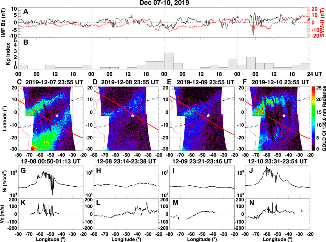
FIGURE 1. (A,B) Interplanetary magnetic field (IMF) Bz, longitudinally symmetric index (SYM-H), and Kp index variations during December 07–10, 2019. (C–F) GOLD nighttime ultraviolet images of OI 135.6 nm emission radiance at 23:55 UT on December 07–10, respectively. The Sao Luis ionosonde (white star), overlapping ICON orbit (red line), and the geomagnetic equator (black dashed line) are also marked. (G–N) Corresponding longitudinal profiles of ICON IVM plasma density and vertical drift.
Nevertheless, the low-latitude ionospheric morphology in the American sector, especially the postsunset EPBs activity, exhibited considerable day-to-day variation, even though there was no hint of a geomagnetic storm or substorm onset within a few hours before local dusk. Figures 1C–F show the GOLD nighttime ultraviolet images of OI 135.6 nm radiance at 23:55 UT on December 07–10, respectively, overlapping with ICON orbital path (red line) at close to the same time. Figure 1G–N show the corresponding longitudinal variation of ICON IVM in-situ plasma density and vertical drift measurements. On December 07, we can see from the GOLD image (Figure 1C) the signatures of EIA crests as two bright low-latitude zonal bands that were produced by enhanced oxygen ion emission therein. There were also noticeable meridional dark streaks embedded in the equatorial trough and cut through the EIA crests, manifesting typical EPBs structure with low density and reduced emission. The signature of EPBs can also be captured by ICON-IVM in-situ ion density measurements (Figure 1G) as noticeable plasma bite-outs, which were associated with the strong pre-reversal enhancement (PRE) of large equatorial upward plasma drift of 100 m/s as shown in Figure 1K. For the following two nights, however, the EPBs feature was largely diminished in GOLD images around the same UT interval on December 08 (Figure 1D) and was almost indiscernible on December 09 (Figure 1E). Similarly, the ICON-IVM measurements during these two nights showed relatively low background ion density conditions with no clear plasma bite-outs (Figures 1H, I), although the plasma vertical drift still showed some spontaneous large values of 100 m/s on December 08 (Figure 1L). In contrast, strong EPBs re-appeared the next evening on December 10 that were simultaneously captured by GOLD image (Figure 1F) and ICON-IVM in-situ measurements (Figure 1J), associated with large upward plasma drift (Figure 1N). In conclusion, the coordinated GOLD and ICON measurements collectively showed that there was large day-to-day variability of EPB activity with considerable suppression on certain nights but intensification on other nights within consecutive 4 days under geomagnetic quiet conditions.
Moreover, such a large day-to-day variability of EPBs intensity can also be deduced from local ionosonde measurements. Figure 2 displays a series of ionograms at the equatorial Sao Luis station between 23:30–24:00 UT on 07–10 December 2019, respectively. As can be seen, on December 07 (Figures 2A–D), there were strong diffuse echoes of range-type spread-F traces that spread across the whole F-region, which are typical characteristics suggesting the presence of large-scale ionospheric plasma irregularities that developed via the R-T instability (Abdu, 2001). At the same UT interval on December 08 (Figures 2E–H), the spread-F signatures were still considerable, but the diffuse echoes were less predominant than the previous night and were mainly confined within the bottomside F-region below 350 km virtual heights. Furthermore, on December 09 (Figure 2I–L), there were almost no spread-F features around midnight yet merely some sporadic and limited structures. Nevertheless, on December 10 (Figure 2M–P), significant spread-F signatures were revived in the same UT interval across the whole F-region, which was much stronger than those from the previous two nights but was comparable to that of December 07. These localized ionogram results are generally in agreement with the above-mentioned GOLD and ICON measurements.
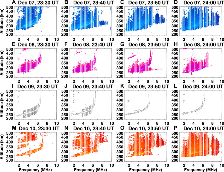
FIGURE 2. (A–P) Sao Luis ionograms during 23:30–24:00 UT on December 07 (blue), 08 (purple), 09 (silver), and 10 (red), 2019, respectively.
Besides ground-based ionosonde measurements and space-borne GOLD/ICON observations, strong day-to-day variation of EPBs can also be observed in GNSS TEC maps. Figures 3A–H show the two-dimensional TEC maps over the South American area at 00:00 and 01:00 UT on 08–11 December 2019, respectively. Considering GOLD has no nighttime measurements after 00:25 UT, we here include the TEC map at a slightly later interval of 01 UT to fill the data gap and illustrate the bubble evolution more clearly. As can be seen, significant EPBs occurred on December 08 (Figures 3A, E) as depletion streaks with reduced TEC values that are marked by dashed lines perpendicular to the geomagnetic equator. In contrast, EPBs features were hardly identified on December 09 (Figures 3B, F) and 10 (Figures 3C, G), yet revived on December 11 (Figures 3D, H) at the same UT intervals. Compared with the surrounding area, the amplitude of the TEC depletion within these EPBs was approximately 5–8 TECU. Moreover, to better identify and trace the temporal evolution of EPBs, Figure 3I–L display the corresponding TEC keogram as a function of time and longitude along −10° latitude between 20 and 04 UT during 07–11 December. As encircled by the black ovals, pronounced postsunset EPBs occurred on December 07–08 (Figure 3I) and 10–11 (Figure 3L), manifesting as parallel comb-like depletion streaks that persisted from 23 to 00 UT to at least 03–04 UT. The inter-bubble distances were estimated to be ∼400–1000 km, which are consistent with typical GOLD observations (e.g., Aa et al., 2020a; Huba and Liu, 2020; Karan et al., 2020). Nevertheless, the EPB intensity on December 08–09 and 09–10 are much weaker and less organized than the first and last days though there were some vague yet blurred streaks.
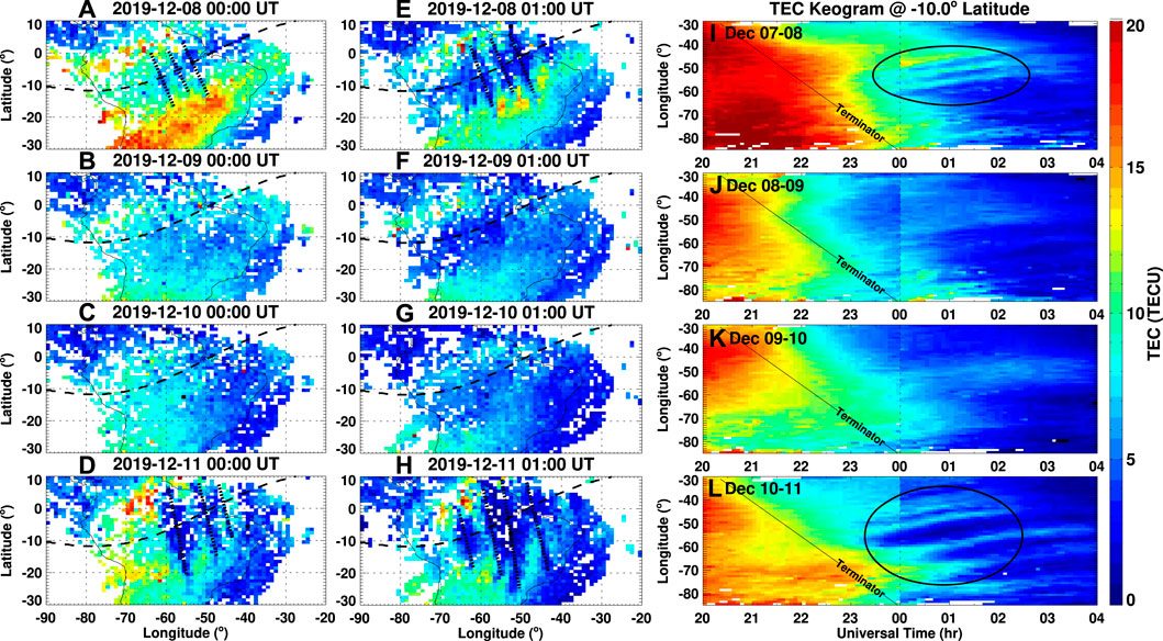
FIGURE 3. (A–H) Gridded TEC maps over the South American area at 00 and 01 UT on 08–11 December 2019, respectively. The geomagnetic equator is marked with a dashed line. The quasi-parallel dotted lines marked strong EPBs. (I–L) TEC keogram as a function of time and longitude along −10° latitude during 07–11 December 2019, respectively. The sunset terminator is marked, and ovals mark strong EPBs.
4 Discussion
4.1 Variation of R-T instability growth rate
To discuss the potential drivers of such large day-to-day variability of EPBs’ intensity, we first examine the R-T instability growth rate variation among the above-mentioned time period of December 07–10, 2019. It is known that Eq. 1 and its derivatives have been widely used in numerical simulations to estimate the flux-tube integrated R-T instability growth rate (e.g., Sultan, 1996; Wu, 2015). However, in order to maximize the usage of realistic observations and avoid the disadvantage of lack of measurements along the flux tube, we here adopt Equation 25 in Sultan (1996) to calculate the local R-T instability growth rate at bottomside F-region around the geomagnetic equator:
where γ is the R-T instability growth rate; E and B are the zonal electric field and geomagnetic field magnitude, respectively; g is the gravitational acceleration; vin is the ion-neutral collision frequency; n0 is the background F-region electron density; z is the altitude. This equation has been proved as an effective approximation to estimate the local linear growth rate of R-T instability near the geomagnetic equator, though its value might be slightly larger than those using flux-tube integrated quantities (e.g., Kelley, 1989; Otsuka, 2018; Das et al., 2021). Note that the meridional neutral wind term is not included in this simplified equation, partially because the nearly parallel-to-B wind in the magnetic meridional plane does not effectively change the conductivity around the equatorial area due to small dip angles therein. The recombination damping term is also excluded since the recombination damp is suggested to be not quite effective (Huba et al., 1996). Other flux-tube terms, such as the integrated Pedersen conductivity in the F-region and E-region, are less likely subject to significant day-to-day variability and thus will not be discussed in the current study.
We here adopted a similar method as indicated by Das et al. (2021) and Kelley (1989) to calculate these parameters. Specifically, the velocity factor (E/B) is replaced by the vertical plasma drift, that is, given by Doppler drift mode measurements of Sao Luis digisonde; the inverse vertical gradient scale length of electron density, 1/n0 (∂n0/∂z), is calculated from the bottomside electron density profile of Sao Luis digisonde. The ion-neutral collision frequency vin is derived from Kelley (1989) as follows:
where nn and ni refer to neutral and ion density. The variable A denotes the mean neutral molecular mass in atomic mass units. These parameters are calculated using NRLMSISE-00 model (Picone et al., 2002). For more details about the mathematical description, readers may refer to Kelley (1989).
Figures 4A, B show Sao Luis ionosonde measurements of electron density profiles and F2-layer peak height (hmF2) as well as F-layer vertical plasma drift with error bars during December 07–10, 2019. Figure 4C displays the corresponding temporal variation of the local linear growth rate of R-T instability derived using Eq. 2 based on those Sao Luis ionosonde measurements. In general, the R-T instability growth rate is larger around nighttime, with peak values typically appearing in the postsunset hours around 19–22 LT (22–01 UT) due to the equatorial PRE effect of the uplifted ionosphere as well as the large density gradient in the bottomside F-region after local sunset and decaying of E-region, as previously interpreted in the Introduction section. Besides this typical diurnal variation pattern, one important question is whether the R-T instability growth rate also experienced similar day-to-day variability in the postsunset evening hours as that of observed EPBs activity among these days. We here compare the magnitude and timing when γ reached peak value in each evening among these 4 days: which are 15 × 10−4 around 22:30 UT (December 07), 18 × 10−4 around 22:30 UT (December 08), 25 × 10−4 around 00:50 + 1 UT (December 09), and 22 × 10−4 around 22:50 UT (December 10), respectively. As can be seen, the day-to-day variation of the peak magnitude of the R-T instability growth rate does not have a strict one-to-one relationship with observed EPBs intensity. For instance, the postsunset peak intensity of γ in the middle 2 days are comparable or even slightly larger than those of the first and fourth days, yet the EPB activity was much more suppressed in the middle 2 days as shown in Figures 1–3. Moreover, the peak value of γ was the smallest on December 07 among those days, while the EPBs intensity on that day is considerably stronger than on December 08 and 09. It is worth noting that, on December 09–10, γ reached its peak value at a later time around 00:50 UT about 2 h later than the other evenings, which might partially explain the inhibited EPBs on that day due to this timing difference. However, it should also be noted that the peak intensity of γ (∼ 25 × 10−4) at this time was the highest in the same UT interval among those days, while the TEC keogram in Figure 3G showed that the nighttime EPB activity even after 01 UT on December 10 was still weaker compared with other nights. Therefore, such a complicated day-to-day variability of EPBs can hardly be explained if solely considering the day-to-day variation of R-T instability growth rate. Some other parameters, such as the seeding factor of TID/AGWs, might also play an indispensable role in causing the observed day-to-day variability of EPBs in this event.
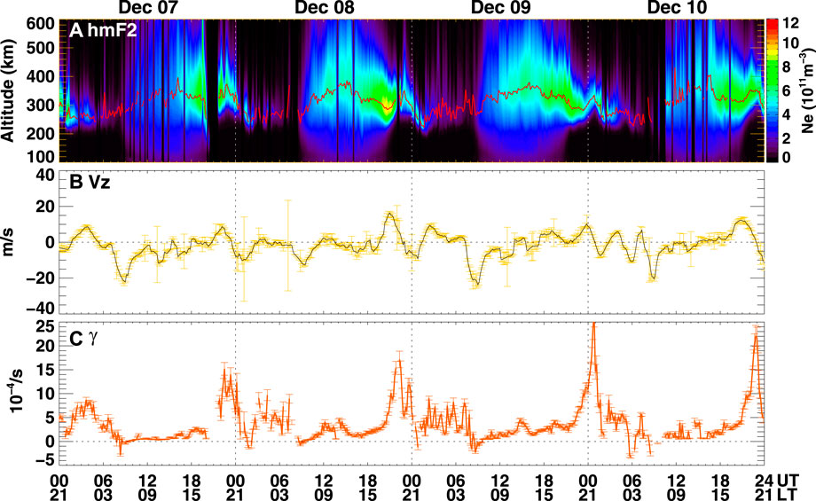
FIGURE 4. Sao Luis ionosonde measurements of (A) electron density profiles and F2-layer peak height (hmF2) as well as (B) F-layer vertical plasma drift with error bars during December 07–10, 2019. (C) Temporal variation of the corresponding linear growth rate of R-T instability.
4.2 TIDs/AGWs activities
We next discuss the background ionospheric conditions in terms of wave structures to investigate the possible seeding effect due to the presence of AGWs on these days. Figure 5 shows four detrended TEC keogram as a function of time and longitude along −10 ∼−20° latitude around the observed EPBs region during 07–10 December 2019, respectively. During the evening of December 07 (Figure 5A) and December 10 (Figure 5D), there were noticeable wavelike fluctuations of medium-scale TID features that propagated eastward during 23–05 UT between −70 ∼−40° longitudes. These TID structures are sometimes considered a proxy that may represent ionospheric signatures of AGWs. The zonal propagating velocity of TID wavefronts is estimated to be around 80–100 m/s, which is generally consistent with the background EPB drifting speed derived from ultraviolet measurements given by previous studies (e.g., Immel et al., 2003; Park et al., 2007; Karan et al., 2020). Moreover, the wavelength of TIDs was estimated to be around a few hundred kilometers, which is generally smaller than the inter-bubble distances. These TIDs were sometimes embedded in the bubbles and were much more evenly distributed across latitudes than bubbles. These TIDs represent medium-scale wave structures that are different from the large-scale bubbles themselves but were present concurrently with the bubbles. In contrary to these two nights with strong TIDs, the TID intensities in the same UT interval were weak during the evening on December 08 (Figure 5B) and were significantly suppressed on December 09 (Figure 5C) as marked by the red oval. This lacking of ionospheric wave structures is in agreement with the observations of inhibited EPBs during the same nights.
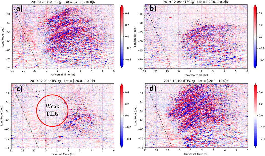
FIGURE 5. (A–D) Detrended TEC keogram as a function of time and longitude along −10 ∼-20° latitude during 07–10 December 2019, respectively. The sunset terminator is marked with a dashed line. The red oval marks relatively weak TID intensity in panel c.
To better check the AGW activities, Figure 6 shows the temporal variation of F-layer true heights at different plasma frequencies (2.0–7.0 MHz) at Fortaleza ionosonde between 21 and 03 UT (18–24 LT) during December 07–10. Here we use Fortaleza as a substitute since there are some data gaps in the Sao Luis results. On December 07 (Figure 6A) and December 10 (Figure 6D), there were identifiable downward phase propagation trends that were marked with dashed lines suggesting the possible presence of AGWs in the upper atmosphere during these two nights (Abdu et al., 2009), while such a downward phase propagation pattern was not so noticeable on December 08 and 09 (Figures 6B, C). This is consistent with those of detrended TEC results. Thus, this coincidence of strong (weak) TID/AGW characteristics together with enhanced (suppressed) EPB activities on the same night collectively illustrate a potential connection between the background wave structures and the development of EPBs. As previously described in the Introduction section, these ionospheric wave structures could not only provide important initial seed perturbations but also large undulation and upwelling of the equatorial F-layer to destabilize the density gradient. Therefore, the stronger (weaker) magnitude the background perturbations have, the less (more) R-T instability growth rate is needed to amplify the fluctuations into the non-linear regime, and the plasma bubbles will be more efficient (inefficient) to be developed (Huang and Kelley, 1996; Retterer and Roddy, 2014). For instance, in the evening of December 09–10, the TID/AGW activity was much weaker than the other nights, and the R-T instability growth rate reached a peak value more than 2 hours later than the other nights. Thus, the combination of these insufficient seeding perturbations and delayed catalyzing factors collectively caused the significant inhibition of EPBs at that night.
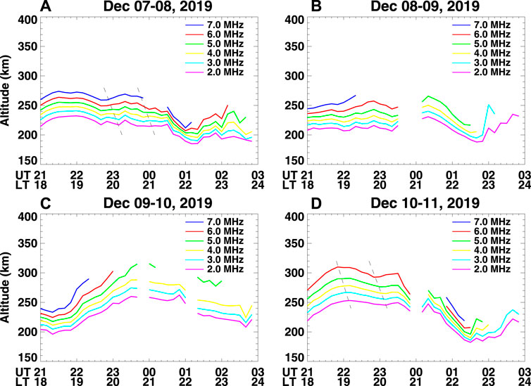
FIGURE 6. (A–D) Temporal variation of F-layer true heights for different frequencies between 2 and 7 MHz at Fortaleza station during 07–11 December 2019, respectively.
Last but not least, we briefly examine the thermospheric neutral wind variation during the selected period of December 07–10, 2019. Figure 7 shows the ICON-MIGHTI observation tracks and corresponding local time, zonal wind, and meridional wind profiles for consecutive orbits focusing on the American sector between 21 and 24 UT that was slightly prior to the observed EPBs on December 07 (Figures 7A–F), December 08 (Figures 7G–L), December 09 (Figure 7M–R), and December 10 (Figures 7S–X), 2019, respectively. Although the zonal and meridional winds showed generally similar longitudinal distribution patterns with comparable amplitudes among these 4 days, there were still some discernible day-to-day differences. In particular, the horizontal winds on December 07 exhibited large wavelike fluctuations of 100 m/s that were associated with a downward phase propagation trend, especially in Figures 7C, E as marked by the parallel dotted lines. Such strong neutral wind perturbations with a downward phase propagation trend are considered to be signatures of traveling atmospheric disturbances (TADs) due to the modulation of upward propagating AGWs from the lower atmosphere, though the latitude-longitude variations were also mixed with such altitudinal variations. In comparison, the wind profiles on other days also have some moderate oscillations though not as strong as that on December 07. Recall from Figure 4 that the peak value of the linear R-T instability growth rate on December 07 was the smallest for the same postsunset period among those consecutive 4 days, while the postsunset EPB intensity on December 07 was much stronger than the following 2 days as shown in Figures 1–3. This could be possibly related to considerable initial seeding perturbations on December 07 caused by those strong neutral wind fluctuations possibly due to AGWs, which can create polarization electric fields to modulate plasma density via E×B drift and/or directly cause plasma perturbation along the geomagnetic field via ion-neutral collision (e.g., Tsunoda et al., 2010; Krall et al., 2013; Zhang et al., 2021). Such important seeding perturbations could be a necessary prerequisite to effectively compensate for the modest strength of the R-T instability growth rate and thus facilitate the development of EPBs on December 07, otherwise, it would be a more inefficient process if irregularities were to develop from merely noise-like small background fluctuations even with relatively large R-T instability growth rate (Retterer and Roddy, 2014), as was likely the cases for December 08 and 09. It is worth noting that the observed wind oscillations are not exactly around the equatorial area due to MIGHTI’s north-looking remote sensing geometry, plus that there were some nighttime data gaps in MIGHTI. However, it is still reasonable to deduce a similar conclusion from the TID/AGWs results shown by the detrended TEC and ionosonde measurements in Figure 6 and Figure 7. A future theoretical simulation is needed to further quantify the neutral wind contribution, which is beyond the scope of the current study.
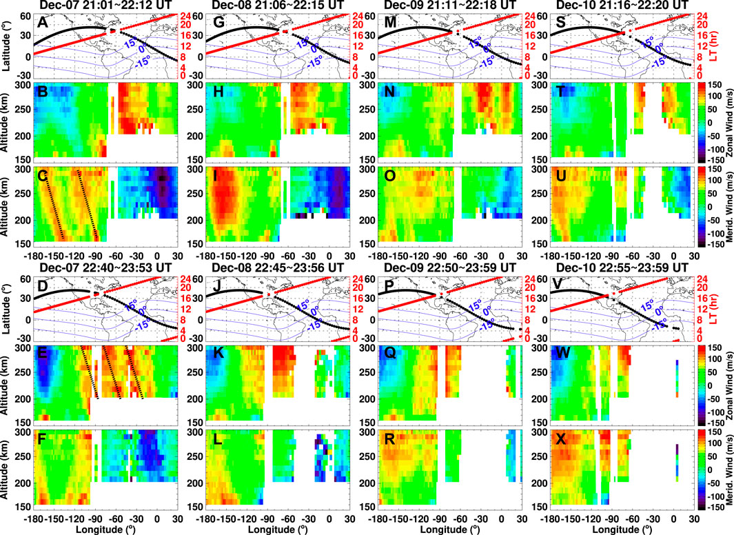
FIGURE 7. ICON MIGHTI observation tracks and corresponding local time, zonal wind (positive eastward), and meridional wind (positive northward) profiles for two consecutive orbits over American sector between 21 and 24 UT on December 07 (A–F), December 08 (G–L), December 09 (M–R), and December 10 (S–X), 2019, respectively. The geomagnetic dip equator and ± 15° latitudes are shown by blue lines. The parallel dotted lines in (C,E) mark large neutral wind oscillations with a downward phase propagation trend.
5 Summary and conclusion
In this study, we conducted a multi-instrument analysis of the day-to-day variability of EPBs over the American sector and potential drivers under a geomagnetically quiet period on 07–10 December 2019. We coordinately utilized GOLD ultraviolet nighttime disk measurements, ICON IVM in-situ plasma and MIGHTI remote sensing wind measurements, ground-based GNSS TEC observations, as well as ionosonde datasets. The main findings and conclusions are as follows:
1) The intensity of postsunset EPBs exhibited a large day-to-day variation in the same UT intervals around 23–03 UT (20–24 LT) during December 07–10. In particular, the EPBs and spread-F irregularity signatures were quite noticeable on the evening of December 07, yet considerably suppressed on December 08, and almost completely inhibited on December 09, then dramatically revived and enhanced on December 10.
2) The day-to-day variation of the local R-T instability growth rate γ), derived using some actual observations via a simple approach, does not have an exact one-to-one relationship with the observed EPBs intensity. Specifically, the peak magnitude and timing of postsunset R-T instability growth rate among those consecutive four nights of December 07–10 was 15 × 10−4/s at 22:30 UT, 18 × 10−4/s at 22:30 UT, 25 × 10−4/s at 00:50 UT, and 22 × 10−4/s at 22:50 UT, respectively. Compared with other evenings, there was a 2-h delay on December 09 when γ reached its peak value, which might partially explain the inhibited EPBs on that night due to this timing difference.
3) The day-to-day variation of TID/TADs feature has a much better agreement with EPBs’ activity: there were relatively strong wavelike perturbations preceded and/or accompanying the considerable EPBs on December 07 and 10, whereas relatively weak wave fluctuations occurred on December 08 and 09 corresponding to EPB inhibition despite of large γ values. These TID/TADs structures are a proxy of atmospheric waves in the upper atmosphere, which played an important seeding role that could effectively compensate for the modest strength of R-T instability growth rate in facilitating the development of EPBs (e.g., December 07). To the contrary, the instability growth would be a more inefficient process if EPBs were to develop from merely small fluctuations of background thermosphere and ionosphere conditions even with a relatively large yet delayed peak value of R-T instability growth rate (e.g., December 09).
Our new results indicate that certain seeding factors due to wave activity in the ionosphere/thermosphere can make an important contribution to EPBs’ day-to-day variability during geomagnetically quiet time. A future direction is to conduct a longer-term analysis of EPBs’ variation and to analyze the contribution of drivers from above and below.
Data availability statement
The original contributions presented in the study are included in the article/Supplementary Material, further inquiries can be directed to the corresponding author.
Author contributions
EA was responsible for the scientific analysis of the observational results, preparing the manuscript, and organizing team efforts. S-RZ was responsible for differential TEC derivation. AC was responsible for GNSS data management. PE contributed substantially to manuscript development. WR was responsible for software development of GNSS data processing and daily GNSS data processing. All members contributed to science discussion and manuscript development.
Funding
GNSS TEC data are part of the United States NSF Geospace Facility program under a cooperative agreement AGS-1952737 with the Massachusetts Institute of Technology. We acknowledge NSF awards AGS-2033787, AGS-2149698, PHY-2028125, and NSFC41974184, NASA support 80NSSC22K0171, 80NSSC21K1310, 80NSSC21K1775, 80NSSC19K0834, and 80GSFC22CA011, AFOSR MURI Project FA9559-16-1-0364, and ONR Grant N00014-17-1-2186 and N00014-22-1-2284.
Acknowledgments
Data for the TEC processing is provided from the following organizations: The Crustal Dynamics Data Information System (CDDIS), the Scripps Orbit and Permanent Array Center (SOPAC), the Continuously Operating Reference System (CORS), the EUREF Permanent GNSS network (EPN), the University NAVSTAR Consortium (UNAVCO), Institut Geographique National in France (IGN), the Brazilian Network for Continuous Monitoring (RBMC), National Geodetic Survey, Instituto Brasileiro de Geografia e Estat
Conflict of interest
The authors declare that the research was conducted in the absence of any commercial or financial relationships that could be construed as a potential conflict of interest.
Publisher’s note
All claims expressed in this article are solely those of the authors and do not necessarily represent those of their affiliated organizations, or those of the publisher, the editors and the reviewers. Any product that may be evaluated in this article, or claim that may be made by its manufacturer, is not guaranteed or endorsed by the publisher.
References
Aa, E., Huang, W., Liu, S., Ridley, A., Zou, S., Shi, L., et al. (2018). Midlatitude plasma bubbles over China and adjacent areas during a magnetic storm on 8 september 2017. Space Weather 16, 321–331. doi:10.1002/2017SW001776
Aa, E., Zou, S., Ridley, A., Zhang, S., Coster, A. J., Erickson, P. J., et al. (2019). Merging of storm time midlatitude traveling ionospheric disturbances and equatorial plasma bubbles. Space Weather 17, 285–298. doi:10.1029/2018SW002101
Aa, E., Zou, S., Eastes, R., Karan, D. K., Zhang, S.-R., Erickson, P. J., et al. (2020a). Coordinated ground-based and space-based observations of equatorial plasma bubbles. J. Geophys. Res. Space Phys. 125, e27569. doi:10.1029/2019JA027569
Aa, E., Zou, S., and Liu, S. (2020b). Statistical analysis of equatorial plasma irregularities retrieved from swarm 2013-2019 observations. J. Geophys. Res. Space Phys. 125, e27022. doi:10.1029/2019JA027022
Abdu, M. A., de Medeiros, R. T., and Sobral, J. H. A. (1982). Equatorial spread F instability conditions as determined from ionograms. Geophys. Res. Lett. 9, 692–695. doi:10.1029/GL009i006p00692
Abdu, M. A., de Medeiros, R. T., Bittencourt, J. A., and Batista, I. S. (1983). Vertical ionization drift velocities and range type spread F in the evening equatorial ionosphere. J. Geophys. Res. 88, 399–402. doi:10.1029/JA088iA01p00399
Abdu, M. A., Alam Kherani, E., Batista, I. S., de Paula, E. R., Fritts, D. C., and Sobral, J. H. A. (2009). Gravity wave initiation of equatorial spread F/plasma bubble irregularities based on observational data from the SpreadFEx campaign. Ann. Geophys. 27, 2607–2622. doi:10.5194/angeo-27-2607-2009
Abdu, M. A. (2001). Outstanding problems in the equatorial ionosphere-thermosphere electrodynamics relevant to spread F. J. Atmos. Solar-Terr. Phys. 63, 869–884. doi:10.1016/S1364-6826(00)00201-7
Abdu, M. A. (2019). Day-to-day and short-term variabilities in the equatorial plasma bubble/spread F irregularity seeding and development. Prog. Earth Planet. Sci. 6, 11. doi:10.1186/s40645-019-0258-1
Alfonsi, L., Cesaroni, C., Spogli, L., Regi, M., Paul, A., Ray, S., et al. (2021). Ionospheric disturbances over the Indian sector during 8 september 2017 geomagnetic storm: Plasma structuring and propagation. Space Weather 19, e2020SW002607. doi:10.1029/2020SW002607
Anderson, D. N., Reinisch, B., Valladare, C., Chau, J., and Veliz, O. (2004). Forecasting the occurrence of ionospheric scintillation activity in the equatorial ionosphere on a day-to-day basis. J. Atmos. Solar-Terr. Phys. 66, 1567–1572. doi:10.1016/j.jastp.2004.07.010
Basu, S., Kudeki, E., Basu, S., Valladares, C. E., Weber, E. J., Zengingonul, H. P., et al. (1996). Scintillations, plasma drifts, and neutral winds in the equatorial ionosphere after sunset. J. Geophys. Res. 101, 26795–26809. doi:10.1029/96JA00760
Booker, H. G., and Wells, H. W. (1938). Scattering of radio waves by the F-region of the ionosphere. Terr. Magn. Atmos. Electr. 43, 249. doi:10.1029/TE043i003p00249
Burke, W. J., Gentile, L. C., Huang, C. Y., Valladares, C. E., and Su, S. Y. (2004). Longitudinal variability of equatorial plasma bubbles observed by DMSP and ROCSAT-1. J. Geophys. Res. Space Phys. 109, A12301. doi:10.1029/2004JA010583
Carter, B. A., Yizengaw, E., Retterer, J. M., Francis, M., Terkildsen, M., Marshall, R., et al. (2014). An analysis of the quiet time day-to-day variability in the formation of postsunset equatorial plasma bubbles in the Southeast Asian region. J. Geophys. Res. Space Phys. 119, 3206–3223. doi:10.1002/2013JA019570
Cherniak, I., and Zakharenkova, I. (2016). First observations of super plasma bubbles in Europe. Geophys. Res. Lett. 43, 11,137–11,145. doi:10.1002/2016GL071421
Chou, M.-Y., Pedatella, N. M., Wu, Q., Huba, J. D., Lin, C. C. H., Schreiner, W. S., et al. (2020). Observation and simulation of the development of equatorial plasma bubbles: Post-sunset rise or upwelling growth? J. Geophys. Res. Space Phys. 125, e28544. doi:10.1029/2020JA028544
Cohen, R., and Bowles, K. L. (1961). On the nature of equatorial spread F. J. Geophys. Res. 66, 1081–1106. doi:10.1029/JZ066i004p01081
Das, S. K., Patra, A. K., Kherani, E. A., Chaitanya, P. P., and Niranjan, K. (2020). Relationship between presunset wave structures and interbubble spacing: The seeding perspective of equatorial plasma bubble. J. Geophys. Res. Space Phys. 125, e28122. doi:10.1029/2020JA028122
Das, S. K., Patra, A. K., and Niranjan, K. (2021). On the assessment of day-to-day occurrence of equatorial plasma bubble. J. Geophys. Res. Space Phys. 126, e2021JA029129. doi:10.1029/2021JA029129
Eastes, R. W., McClintock, W. E., Burns, A. G., Anderson, D. N., Andersson, L., Codrescu, M., et al. (2017). The global-scale observations of the limb and disk (GOLD) mission. Space Sci. Rev. 212, 383–408. doi:10.1007/s11214-017-0392-2
Eastes, R. W., Solomon, S. C., Daniell, R. E., Anderson, D. N., Burns, A. G., England, S. L., et al. (2019). Global-scale observations of the equatorial ionization anomaly. Geophys. Res. Lett. 46, 9318–9326. doi:10.1029/2019GL084199
Eastes, R. W., McClintock, W. E., Burns, A. G., Anderson, D. N., Andersson, L., Aryal, S., et al. (2020). Initial observations by the GOLD mission. J. Geophys. Res. Space Phys. 125, e27823. doi:10.1029/2020JA027823
Eccles, J. V., St. Maurice, J. P., and Schunk, R. W. (2015). Mechanisms underlying the prereversal enhancement of the vertical plasma drift in the low-latitude ionosphere. J. Geophys. Res. Space Phys. 120, 4950–4970. doi:10.1002/2014JA020664
Farley, D. T., Bonelli, E., Fejer, B. G., and Larsen, M. F. (1986). The prereversal enhancement of the zonal electric field in the equatorial ionosphere. J. Geophys. Res. 91, 13723–13728. doi:10.1029/JA091iA12p13723
Fejer, B. G., Scherliess, L., and de Paula, E. R. (1999). Effects of the vertical plasma drift velocity on the generation and evolution of equatorial spread F. J. Geophys. Res. 104, 19859–19869. doi:10.1029/1999JA900271
Fukao, S., Yokoyama, T., Tayama, T., Yamamoto, M., Maruyama, T., and Saito, S. (2006). Eastward traverse of equatorial plasma plumes observed with the Equatorial Atmosphere Radar in Indonesia. Ann. Geophys. 24, 1411–1418. doi:10.5194/angeo-24-1411-2006
Harding, B. J., Makela, J. J., Englert, C. R., Marr, K. D., Harlander, J. M., England, S. L., et al. (2017). The MIGHTI wind retrieval algorithm: Description and verification. Space Sci. Rev. 212, 585–600. doi:10.1007/s11214-017-0359-3
Heelis, R. A., Crowley, G., Rodrigues, F., Reynolds, A., Wilder, R., Azeem, I., et al. (2012). The role of zonal winds in the production of a pre-reversal enhancement in the vertical ion drift in the low latitude ionosphere. J. Geophys. Res. Space Phys. 117, A08308. doi:10.1029/2012JA017547
Heelis, R. A., Stoneback, R. A., Perdue, M. D., Depew, M. D., Morgan, W. A., Mankey, M. W., et al. (2017). Ion velocity measurements for the ionospheric connections explorer. Space Sci. Rev. 212, 615–629. doi:10.1007/s11214-017-0383-3
Heelis, R. A. (2004). Electrodynamics in the low and middle latitude ionosphere: A tutorial. J. Atmos. Solar-Terr. Phys. 66, 825–838. doi:10.1016/j.jastp.2004.01.034
Huang, C.-S., and Hairston, M. R. (2015). The postsunset vertical plasma drift and its effects on the generation of equatorial plasma bubbles observed by the C/NOFS satellite. J. Geophys. Res. Space Phys. 120, 2263–2275. doi:10.1002/2014JA020735
Huang, C.-S., and Kelley, M. C. (1996). Nonlinear evolution of equatorial spread F. 2. Gravity wave seeding of Rayleigh-Taylor instability. J. Geophys. Res. 101, 293–302. doi:10.1029/95JA02210
Huang, C.-S., de La Beaujardiere, O., Roddy, P. A., Hunton, D. E., Ballenthin, J. O., and Hairston, M. R. (2012). Generation and characteristics of equatorial plasma bubbles detected by the C/NOFS satellite near the sunset terminator. J. Geophys. Res. Space Phys. 117, A11313. doi:10.1029/2012JA018163
Huba, J. D., and Joyce, G. (2010). Global modeling of equatorial plasma bubbles. Geophys. Res. Lett. 37, L17104. doi:10.1029/2010GL044281
Huba, J. D., and Krall, J. (2013). Impact of meridional winds on equatorial spread F: Revisited. Geophys. Res. Lett. 40, 1268–1272. doi:10.1002/grl.50292
Huba, J. D., and Liu, H. L. (2020). Global modeling of equatorial spread F with SAMI3/WACCM-X. Geophys. Res. Lett. 47, e88258. doi:10.1029/2020GL088258
Huba, J. D., Bernhardt, P. A., Ossakow, S. L., and Zalesak, S. T. (1996). The Rayleigh-Taylor instability is not damped by recombination in the F region. J. Geophys. Res. 101, 24553–24556. doi:10.1029/96JA02527
Huba, J. D., Joyce, G., and Krall, J. (2008). Three-dimensional equatorial spread F modeling. Geophys. Res. Lett. 35, L10102. doi:10.1029/2008GL033509
Hysell, D. L., and Burcham, J. D. (2002). Long term studies of equatorial spread/F using the JULIA radar at Jicamarca. J. Atmos. Solar-Terr. Phys. 64, 1531–1543. doi:10.1016/S1364-6826(02)00091-3
Hysell, D. L. (2000). An overview and synthesis of plasma irregularities in equatorial spread/F. J. Atmos. Solar-Terr. Phys. 62, 1037–1056. doi:10.1016/S1364-6826(00)00095-X
Immel, T. J., Mende, S. B., Frey, H. U., Peticolas, L. M., and Sagawa, E. (2003). Determination of low latitude plasma drift speeds from FUV images. Geophys. Res. Lett. 30, 1945. doi:10.1029/2003GL017573
Immel, T. J., England, S. L., Mende, S. B., Heelis, R. A., Englert, C. R., Edelstein, J., et al. (2018). The ionospheric connection explorer mission: Mission goals and design. Space Sci. Rev. 214, 13. doi:10.1007/s11214-017-0449-2
Jin, H., Zou, S., Chen, G., Yan, C., Zhang, S., and Yang, G. (2018). Formation and evolution of low-latitude F region field-aligned irregularities during the 7-8 september 2017 storm: Hainan coherent scatter phased Array radar and digisonde observations. Space Weather 16, 648–659. doi:10.1029/2018SW001865
Karan, D. K., Daniell, R. E., England, S. L., Martinis, C. R., Eastes, R. W., Burns, A. G., et al. (2020). First zonal drift velocity measurement of equatorial plasma bubbles (EPBs) from a geostationary orbit using GOLD data. J. Geophys. Res. Space Phys. 125, e28173. doi:10.1029/2020JA028173
Kelley, M. C., Larsen, M. F., Lahoz, C., and McClure, J. P. (1981). Gravity wave initiation of equatorial spread F: A case study. J. Geophys. Res. 86, 9087–9100. doi:10.1029/JA086iA11p09087
Kelley, M. C. (1989). “Equatorial plasma instabilities,” in The Earth’s ionosphere: Plasma Physics and electrodynamics. Editor M. C. Kelley (Academic Press), 113–185. doi:10.1016/B978-0-12-404013-7.50009-5
Kil, H., Su, S. Y., Paxton, L. J., Wolven, B. C., Zhang, Y., Morrison, D., et al. (2004). Coincident equatorial bubble detection by TIMED/GUVI and ROCSAT-1. Geophys. Res. Lett. 31, L03809. doi:10.1029/2003GL018696
Kil, H., Paxton, L. J., and Oh, S.-J. (2009). Global bubble distribution seen from ROCSAT-1 and its association with the evening prereversal enhancement. J. Geophys. Res. Space Phys. 114, A06307. doi:10.1029/2008JA013672
Krall, J., Huba, J. D., Joyce, G., and Zalesak, S. T. (2009). Three-dimensional simulation of equatorial spread-F with meridional wind effects. Ann. Geophys. 27, 1821–1830. doi:10.5194/angeo-27-1821-2009
Krall, J., Huba, J. D., and Fritts, D. C. (2013). On the seeding of equatorial spread F by gravity waves. Geophys. Res. Lett. 40, 661–664. doi:10.1002/grl.50144
Kudeki, E., Akgiray, A., Milla, M., Chau, J. L., and Hysell, D. L. (2007). Equatorial spread-F initiation: Post-sunset vortex, thermospheric winds, gravity waves. J. Atmos. Solar-Terr. Phys. 69, 2416–2427. doi:10.1016/j.jastp.2007.04.012
Makela, J. J., and Kelley, M. C. (2003). Field-aligned 777.4-nm composite airglow images of equatorial plasma depletions. Geophys. Res. Lett. 30, 1442. doi:10.1029/2003GL017106
Makela, J. J., Vadas, S. L., Muryanto, R., Duly, T., and Crowley, G. (2010). Periodic spacing between consecutive equatorial plasma bubbles. Geophys. Res. Lett. 37, L14103. doi:10.1029/2010GL043968
Martinis, C., Baumgardner, J., Mendillo, M., Wroten, J., Coster, A., and Paxton, L. (2015). The night when the auroral and equatorial ionospheres converged. J. Geophys. Res. Space Phys. 120, 8085–8095. doi:10.1002/2015JA021555
Maruyama, T. (1988). A diagnostic model for equatorial spread F. 1. Model description and application to electric field and neutral wind effects. J. Geophys. Res. 93, 14611–14622. doi:10.1029/JA093iA12p14611
Mendillo, M., and Baumgardner, J. (1982). Airglow characteristics of equatorial plasma depletions. J. Geophys. Res. 87, 7641–7652. doi:10.1029/JA087iA09p07641
Mendillo, M., Meriwether, J., and Biondi, M. (2001). Testing the thermospheric neutral wind suppression mechanism for day-to-day variability of equatorial spread F. J. Geophys. Res. 106, 3655–3663. doi:10.1029/2000JA000148
Otsuka, Y., Shiokawa, K., Ogawa, T., and Wilkinson, P. (2002). Geomagnetic conjugate observations of equatorial airglow depletions. Geophys. Res. Lett. 29, 43-1–43-4. doi:10.1029/2002GL015347
Otsuka, Y. (2018). Review of the generation mechanisms of post-midnight irregularities in the equatorial and low-latitude ionosphere. Prog. Earth Planet. Sci. 5, 57. doi:10.1186/s40645-018-0212-7
Park, S. H., England, S. L., Immel, T. J., Frey, H. U., and Mende, S. B. (2007). A method for determining the drift velocity of plasma depletions in the equatorial ionosphere using far-ultraviolet spacecraft observations. J. Geophys. Res. Space Phys. 112, A11314. doi:10.1029/2007JA012327
Picone, J. M., Hedin, A. E., Drob, D. P., and Aikin, A. C. (2002). NRLMSISE-00 empirical model of the atmosphere: Statistical comparisons and scientific issues. J. Geophys. Res. Space Phys. 107, SIA 15-21–SIA 15-16. doi:10.1029/2002JA009430
Retterer, J. M., and Roddy, P. (2014). Faith in a seed: On the origins of equatorial plasma bubbles. Ann. Geophys. 32, 485–498. doi:10.5194/angeo-32-485-2014
Retterer, J. M., Decker, D. T., Borer, W. S., Daniell, R. E., and Fejer, B. G. (2005). Assimilative modeling of the equatorial ionosphere for scintillation forecasting: Modeling with vertical drifts. J. Geophys. Res. Space Phys. 110, A11307. doi:10.1029/2002JA009613
Rideout, W., and Coster, A. (2006). Automated gps processing for global total electron content data. GPS Solut. 10, 219–228. doi:10.1007/s10291-006-0029-5
Rodrigues, F. S., Hickey, D. A., Zhan, W., Martinis, C. R., Fejer, B. G., Milla, M. A., et al. (2018). Multi-instrumented observations of the equatorial F-region during june solstice: Large-scale wave structures and spread- F. Prog. Earth Planet. Sci. 5, 14. doi:10.1186/s40645-018-0170-0
Röttger, J. (1973). Wave-like structures of large-scale equatorial spread-F irregularities. J. Atmos. Terr. Phys. 35, 1195–1206. doi:10.1016/0021-9169(73)90016-0
Saito, S., and Maruyama, T. (2006). Ionospheric height variations observed by ionosondes along magnetic meridian and plasma bubble onsets. Ann. Geophys. 24, 2991–2996. doi:10.5194/angeo-24-2991-2006
Saito, S., and Maruyama, T. (2007). Large-scale longitudinal variation in ionospheric height and equatorial spread F occurrences observed by ionosondes. Geophys. Res. Lett. 34, L16109. doi:10.1029/2007GL030618
Sarudin, I., Hamid, N. S. A., Abdullah, M., Buhari, S. M., Shiokawa, K., Otsuka, Y., et al. (2021). Influence of zonal wind velocity variation on equatorial plasma bubble occurrences over southeast asia. J. Geophys. Res. Space Phys. 126, e28994. doi:10.1029/2020JA028994
Savitzky, A., and Golay, M. J. E. (1964). Smoothing and differentiation of data by simplified least squares procedures. Anal. Chem. 36, 1627–1639. doi:10.1021/ac60214a047
Shinagawa, H., Jin, H., Miyoshi, Y., Fujiwara, H., Yokoyama, T., and Otsuka, Y. (2018). Daily and seasonal variations in the linear growth rate of the Rayleigh-Taylor instability in the ionosphere obtained with GAIA. Prog. Earth Planet. Sci. 5, 16. doi:10.1186/s40645-018-0175-8
Singh, S., Johnson, F. S., and Power, R. A. (1997). Gravity wave seeding of equatorial plasma bubbles. J. Geophys. Res. 102, 7399–7410. doi:10.1029/96JA03998
Smith, J. M., Rodrigues, F. S., Fejer, B. G., and Milla, M. A. (2016). Coherent and incoherent scatter radar study of the climatology and day-to-day variability of mean F region vertical drifts and equatorial spread F. J. Geophys. Res. Space Phys. 121, 1466–1482. doi:10.1002/2015JA021934
Stolle, C., Lühr, H., Rother, M., and Balasis, G. (2006). Magnetic signatures of equatorial spread F as observed by the CHAMP satellite. J. Geophys. Res. 111, A02304. doi:10.1029/2005JA011184
Su, S. Y., Chao, C. K., and Liu, C. H. (2008). On monthly/seasonal/longitudinal variations of equatorial irregularity occurrences and their relationship with the postsunset vertical drift velocities. J. Geophys. Res. Space Phys. 113, A05307. doi:10.1029/2007JA012809
Sultan, P. J. (1996). Linear theory and modeling of the Rayleigh-Taylor instability leading to the occurrence of equatorial spread F. J. Geophys. Res. 101, 26875–26891. doi:10.1029/96JA00682
Takahashi, H., Taylor, M. J., Pautet, P. D., Medeiros, A. F., Gobbi, D., Wrasse, C. M., et al. (2009). Simultaneous observation of ionospheric plasma bubbles and mesospheric gravity waves during the SpreadFEx Campaign. Ann. Geophys. 27, 1477–1487. doi:10.5194/angeo-27-1477-2009
Takahashi, H., Wrasse, C. M., Otsuka, Y., Ivo, A., Gomes, V., Paulino, I., et al. (2015). Plasma bubble monitoring by TEC map and 630 nm airglow image. J. Atmos. Solar-Terr. Phys. 130, 151–158. doi:10.1016/j.jastp.2015.06.003
Takahashi, H., Wrasse, C. M., Figueiredo, C. A. O. B., Barros, D., Abdu, M. A., Otsuka, Y., et al. (2018). Equatorial plasma bubble seeding by MSTIDs in the ionosphere. Prog. Earth Planet. Sci. 5, 32. doi:10.1186/s40645-018-0189-2
Taori, A., Patra, A. K., and Joshi, L. M. (2011). Gravity wave seeding of equatorial plasma bubbles: An investigation with simultaneous F region, E region, and middle atmospheric measurements. J. Geophys. Res. Space Phys. 116, A05310. doi:10.1029/2010JA016229
Tsunoda, R. T., and White, B. R. (1981). On the generation and growth of equatorial backscatter plumes 1. Wave structure in the Bottomside F layer. J. Geophys. Res. 86, 3610–3616. doi:10.1029/JA086iA05p03610
Tsunoda, R. T., Bubenik, D. M., Thampi, S. V., and Yamamoto, M. (2010). On large-scale wave structure and equatorial spread F without a post-sunset rise of the F layer. Geophys. Res. Lett. 37, L07105. doi:10.1029/2009GL042357
Tsunoda, R. T., Saito, S., and Nguyen, T. T. (2018). Post-sunset rise of equatorial F layer—Or upwelling growth? Prog. Earth Planet. Sci. 5, 22. doi:10.1186/s40645-018-0179-4
Tsunoda, R. T. (2005). On the enigma of day-to-day variability in equatorial spread F. Geophys. Res. Lett. 32, L08103. doi:10.1029/2005GL022512
Tsunoda, R. T. (2010). On equatorial spread F: Establishing a seeding hypothesis. J. Geophys. Res. Space Phys. 115, A12303. doi:10.1029/2010JA015564
Tsunoda, R. T. (2015). Upwelling: A unit of disturbance in equatorial spread F. Prog. Earth Planet. Sci. 2, 9. doi:10.1186/s40645-015-0038-5
Vadas, S. L. (2007). Horizontal and vertical propagation and dissipation of gravity waves in the thermosphere from lower atmospheric and thermospheric sources. J. Geophys. Res. Space Phys. 112, A06305. doi:10.1029/2006JA011845
Valladares, C. E., and Chau, J. L. (2012). The low-latitude ionosphere sensor network: Initial results. Radio Sci. 47, RS0L17. doi:10.1029/2011RS004978
Vankadara, R. K., Panda, S. K., Amory-Mazaudier, C., Fleury, R., Devananboyina, V. R., Pant, T. K., et al. (2022). Signatures of equatorial plasma bubbles and ionospheric scintillations from magnetometer and GNSS observations in the Indian longitudes during the space weather events of early september 2017. Remote Sens. 14, 652. doi:10.3390/rs14030652
Vierinen, J., Coster, A. J., Rideout, W. C., Erickson, P. J., and Norberg, J. (2016). Statistical framework for estimating GNSS bias. Atmos. Meas. Tech. 9, 1303–1312. doi:10.5194/amt-9-1303-2016
Whalen, J. A. (2001). The equatorial anomaly: Its quantitative relation to equatorial bubbles, bottomside spread F, and E×B drift velocity during a month at solar maximum. J. Geophys. Res. 106, 29125–29132. doi:10.1029/2001JA000089
Woodman, R. F., and La Hoz, C. (1976). Radar observations of F region equatorial irregularities. J. Geophys. Res. 81, 5447–5466. doi:10.1029/JA081i031p05447
Wu, Q. (2015). Longitudinal and seasonal variation of the equatorial flux tube integrated Rayleigh-Taylor instability growth rate. J. Geophys. Res. Space Phys. 120, 7952–7957. doi:10.1002/2015JA021553
Xiong, C., Stolle, C., Lühr, H., Park, J., Fejer, B. G., and Kervalishvili, G. N. (2016). Scale analysis of equatorial plasma irregularities derived from Swarm constellation. Earth, Planets Space 68, 121. doi:10.1186/s40623-016-0502-5
Yamamoto, M., Otsuka, Y., Jin, H., and Miyoshi, Y. (2018). Relationship between day-to-day variability of equatorial plasma bubble activity from GPS scintillation and atmospheric properties from Ground-to-topside model of Atmosphere and Ionosphere for Aeronomy (GAIA) assimilation. Prog. Earth Planet. Sci. 5, 26. doi:10.1186/s40645-018-0184-7
Yizengaw, E., and Groves, K. M. (2018). Longitudinal and seasonal variability of equatorial ionospheric irregularities and electrodynamics. Space Weather 16, 946–968. doi:10.1029/2018SW001980
Yokoyama, T., Shinagawa, H., and Jin, H. (2014). Nonlinear growth, bifurcation, and pinching of equatorial plasma bubble simulated by three-dimensional high-resolution bubble model. J. Geophys. Res. Space Phys. 119, 10,474–10,482. doi:10.1002/2014JA020708
Yokoyama, T., Jin, H., Shinagawa, H., and Liu, H. (2019). Seeding of equatorial plasma bubbles by vertical neutral wind. Geophys. Res. Lett. 46, 7088–7095. doi:10.1029/2019GL083629
Yokoyama, T. (2017). A review on the numerical simulation of equatorial plasma bubbles toward scintillation evaluation and forecasting. Prog. Earth Planet. Sci. 4, 37. doi:10.1186/s40645-017-0153-6
Zakharenkova, I., Astafyeva, E., and Cherniak, I. (2016). GPS and in situ Swarm observations of the equatorial plasma density irregularities in the topside ionosphere. Earth, Planets Space 68, 120. doi:10.1186/s40623-016-0490-5
Zhang, S.-R., Erickson, P. J., Goncharenko, L. P., Coster, A. J., Rideout, W., and Vierinen, J. (2017). Ionospheric bow waves and perturbations induced by the 21 august 2017 solar eclipse. Geophys. Res. Lett. 44, 12,067–12,073. doi:10.1002/2017GL076054
Keywords: equatorial plasma bubbles, Rayleigh-Taylor instability, day-to-day variation, TID/AGWs, GOLD-ICON, GNSS TEC
Citation: Aa E, Zhang S-R, Coster AJ, Erickson PJ and Rideout W (2023) Multi-instrumental analysis of the day-to-day variability of equatorial plasma bubbles. Front. Astron. Space Sci. 10:1167245. doi: 10.3389/fspas.2023.1167245
Received: 16 February 2023; Accepted: 09 March 2023;
Published: 21 March 2023.
Edited by:
Jaroslav Chum, Institute of Atmospheric Physics (ASCR), CzechiaReviewed by:
Tobias Verhulst, Royal Meteorological Institute of Belgium, BelgiumSampad Kumar Panda, K L University, India
Copyright © 2023 Aa, Zhang, Coster, Erickson and Rideout. This is an open-access article distributed under the terms of the Creative Commons Attribution License (CC BY). The use, distribution or reproduction in other forums is permitted, provided the original author(s) and the copyright owner(s) are credited and that the original publication in this journal is cited, in accordance with accepted academic practice. No use, distribution or reproduction is permitted which does not comply with these terms.
*Correspondence: Ercha Aa, YWVyY2hhQG1pdC5lZHU=