 M. Akhavan-Tafti1*
 L. Johnson2
 R. Sood3
 J. A. Slavin1
 T. Pulkkinen1
 S. Lepri1
 E. Kilpua4
 D. Fontaine5A. Szabo6
 L. Wilson6
 G. Le6
 T. Y. Atilaw1
 M. Ala-Lahti1
 S. L. Soni1D. Biesecker6,7
 L. K. Jian6
 D. Lario6
- 1Climate and Space Sciences and Engineering (CLaSP), University of Michigan, Ann Arbor, MI, United States
- 2NASA Marshall Space Flight Center (MSFC), Huntsville, AL, United States
- 3Aerospace Engineering and Mechanics, University of Alabama, Tuscaloosa, AL, United States
- 4Department of Physics, University of Helsinki, Helsinki, Finland
- 5Laboratoire de Physique des Plasmas (LPP), École Polytechnique, Centre National de la Recherche Scientifique, Sorbonne Université, Institut Polytechnique de Paris, Palaiseau, France
- 6NASA Goddard Space Flight Center (GSFC), Greenbelt, MD, United States
- 7NOAA Space Weather Prediction Center (SWPC), Boulder, CO, United States
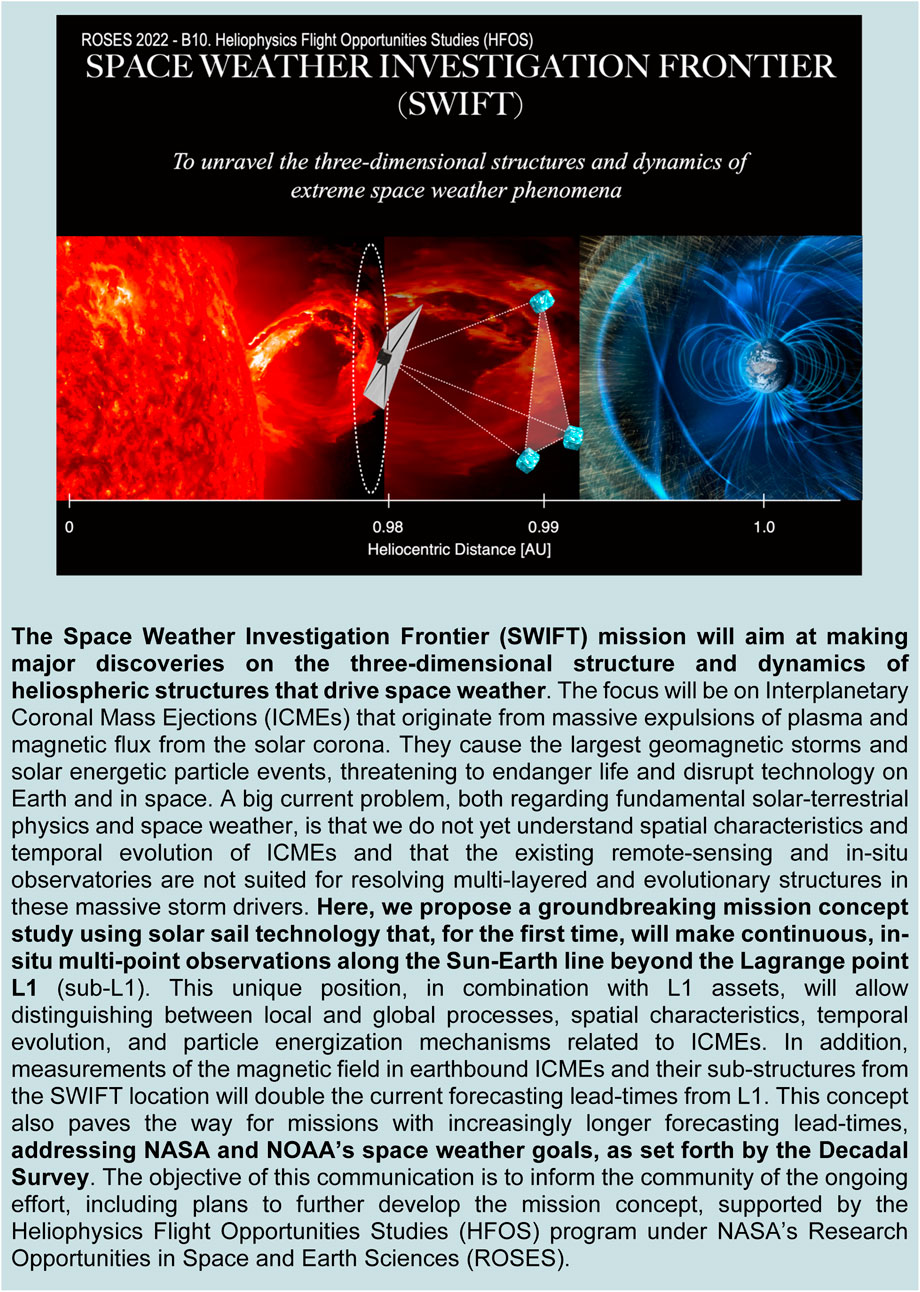
The Space Weather Investigation Frontier (SWIFT) mission will aim at making major discoveries on the three-dimensional structure and dynamics of heliospheric structures that drive space weather. The focus will be on Interplanetary Coronal Mass Ejections (ICMEs) that originate from massive expulsions of plasma and magnetic flux from the solar corona. They cause the largest geomagnetic storms and solar energetic particle events, threatening to endanger life and disrupt technology on Earth and in space. A big current problem, both regarding fundamental solar-terrestrial physics and space weather, is that we do not yet understand spatial characteristics and temporal evolution of ICMEs and that the existing remote-sensing and in-situ observatories are not suited for resolving multi-layered and evolutionary structures in these massive storm drivers. Here, we propose a groundbreaking mission concept study using solar sail technology that, for the first time, will make continuous, in-situ multi-point observations along the Sun-Earth line beyond the Lagrange point L1 (sub-L1). This unique position, in combination with L1 assets, will allow distinguishing between local and global processes, spatial characteristics, temporal evolution, and particle energization mechanisms related to ICMEs. In addition, measurements of the magnetic field in earthbound ICMEs and their sub-structures from the SWIFT location will double the current forecasting lead-times from L1. This concept also paves the way for missions with increasingly longer forecasting lead-times, addressing NASA and NOAA’s space weather goals, as set forth by the Decadal Survey. The objective of this communication is to inform the community of the ongoing effort, including plans to further develop the mission concept, supported by the Heliophysics Flight Opportunities Studies (HFOS) program under NASA’s Research Opportunities in Space and Earth Sciences (ROSES).
1 Introduction
1.1 Interplanetary coronal mass ejections
Coronal mass ejections (CMEs), which are massive expulsions of plasma and magnetic flux, originate from the solar corona and propagate into interplanetary space with speeds up to 3,000 km/s. The occurrence rate of CMEs is dependent on the solar cycle, ranging between 1 per day at solar minimum to 5 per day during solar maximum (Webb and Howard, 2012). CMEs are the main drivers of extreme space weather effects at Earth, considered the main cause of major geomagnetic storms. Their detrimental impacts include disrupting satellite operations, navigation systems, radio communications and ground power grids (Schrijver et al., 2015).
Interplanetary coronal mass ejections (ICMEs) are traditionally envisioned as expanding flux ropes (Burlaga et al., 1981; Klein and Burlaga, 1982; Marubashi, 1986; Lepping, Burlaga, and Jones, 1990). They are believed to be still magnetically attached to the Sun at both ends. As ICME propagate through the ambient solar wind plasma and magnetic field in the interplanetary medium, they often form a leading shock, as illustrated in Figure 1. While instructive, this simplified picture of an ICME and its coronal connection has informed in-situ observation interpretations, heliospheric models, and geomagnetic-storm predictions (Gonzalez and Tsurutani, 1987; Wilson, 1987; Russell et al., 2000). However, remote-sensing observations and in-situ measurements from vantage points have shown that the ICME evolution from the solar corona to 1AU may substantially diverge from the self-similar flux-rope expansion picture.
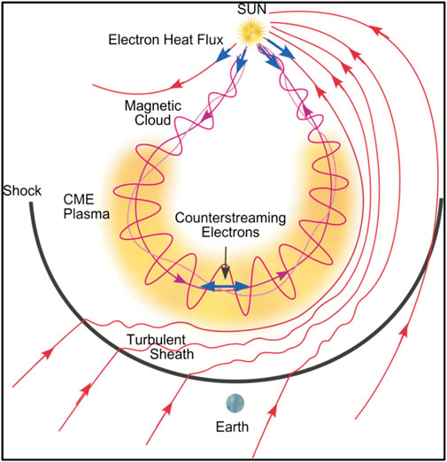
FIGURE 1. A “standard” ICME includes a leading shock, a compressed ambient solar-wind “sheath” where the magnetic field may be perturbed by the shock and foreshock, and a shock “driver” consisting of a magnetic cloud with a flux rope-like magnetic-field structure. Image courtesy of Zurbuchen and Richardson (2006).
STEREO launched in 2006, has provided the heliophysics community a unique and revolutionary view of the Sun-Earth system. Heliospheric images (HI) from STEREO/HI-2 have revealed detailed spatial structures within interplanetary CMEs, including leading-edge pileup, interior cavities, filamentary structure, and rear cusps (DeForest et al., 2011). Various techniques have been developed that enable the spatial locations and propagation directions of CMEs to be inferred, based on fitting their moving radiance patterns (e.g., Davies et al., 2012). With the STEREO/SECCHI package, a CME can be remotely imaged from its nascent stage in the inner corona all the way out to 1 AU and beyond (e.g., Harrison et al., 2008). However, understanding the structural characteristics of ICMEs requires quantitative in situ particle and field measurements from a plurality of well-separated probes, to constrain physical models.
1.2 Simple evolution of interplanetary coronal mass ejections
Single-spacecraft observations have indicated that some ICMEs are simple in structure and evolve self-similarly up to 1 AU, therefore current physical models are successful in determining their characteristics and geo-effectiveness. For example, Davies et al. (2021) reported the in-situ detection of an ICME on 19 April 2020 by Solar Orbiter (SolO) at a heliocentric distance of 0.809 AU. The ICME was later observed (SolO+20.5 h) by Wind near the Sun-Earth Lagrange point L1 at 0.996 AU. Figure 2 provides an overview of magnetic field and spacecraft locations. Figures 2F, G further provides a model of the ICME flux rope using the 3DCORE flux rope modeling technique (Weiss et al., 2021a), assuming a 3D torus-like structure anchored on the surface of the Sun which expands self-similarly during its propagation throughout the heliosphere. The scaling factor between SolO and Wind magnetic field components is close to unity, indicating that the flux rope or magnetic cloud (MC) underwent little to no expansion as it propagated beyond 0.8 AU to L1. However, the authors show that the ICME sheath region sharply expanded (+64%), while the magnetic field magnitude dropped (B ∝ r−2). Similarly, Nieves-Chinchilla et al. (2022) reported the “elastic” interaction of two ICMEs wherein the two ICMEs survived the collision, resulting only in a momentum exchange. A radial distribution of well-separated probes will provide boundary constraints for simple ICME models.
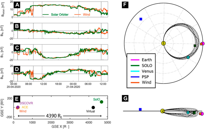
FIGURE 2. (A–D) Magnetic field measurements at Wind (orange) and Solar Orbiter (green). The vertical dashed (dotted) lines constrain the (unperturbed) flux rope. (E) The spatial distribution of L1 observatories and SolO in geocentric solar ecliptic (GSE) coordinates (F) top-down and (G) side views of the 3DCORE geometry within the solar system up to 1 AU. Image courtesy of Davies et al. (2021).
1.3 Complex evolution of interplanetary coronal mass ejections
By contrast, the structure, evolution, and geo-effectiveness of complex ICMEs are very difficult to predict, due to both the complexity of the processes that occur at the Sun during the CME emergence, and specially the various processes that occur during CMEs’ propagation through the interplanetary space. Various aspects of the ICME geo-effectiveness have been previously studied, including the formation of shocks and sheaths (Gosling, 1990), the CME dynamics in the solar corona (Möstl et al., 2010; Owens et al., 2012), as well as compression effects at their back owing to trailing high-speed solar wind streams (Fenrich and Luhmann, 1998; Rouillard et al., 2010a).
The ICME evolution from the solar corona to 1AU and beyond (Gosling J. T. et al., 2006) has been repeatedly shown to substantially differ from the self-similar flux-rope expansion picture (Gosling et al., 2005; Fermo et al., 2014). One process responsible for the complex evolution of ICMEs in the interplanetary environment is magnetic reconnection at the front of ICMEs, as demonstrated in Figure 3. Magnetic reconnection, a ubiquitous process in the solar wind (Farrugia et al., 2001; Gosling et al., 2005; Gosling J. T. et al., 2006; Davis et al., 2006; Phan et al., 2006; Huttunen et al., 2008; Eriksson et al., 2009; Lavraud et al., 2009) can rearrange magnetic fields, including, in this case, eroding away part of the magnetic flux impinging on the Earth’s magnetosphere. One of the key signatures of magnetic reconnection is the presence of a velocity jet (Burch et al., 2016), associated with the explosive conversion of magnetic energy to plasma kinetic energy. Magnetic reconnection has been reportedly observed at various key boundaries, including the heliospheric current sheet (Gosling J. T. et al., 2006; Lavraud et al., 2009) and within (Gosling and Szabo, 2008) and at the front boundary of MCs (Ruffenach et al., 2012). Reconnection is particularly frequent in low-β plasma such as the magnetic cloud, even in the presence of a low magnetic shear (Gosling and Szabo, 2008). Lavraud et al. (2014) showed using both in-situ observations and models that MC-erosion due to magnetic reconnection can reduce the geo-effectiveness of a storm by up to 30%, adding that 50% of the erosion likely takes place between the Mercury and Earth’s obits. These findings highlight the critical need for upstream satellites to sample complex ICMEs at various solar radii to further our understanding of the ICME evolution processes as well as the corresponding geo-effectiveness in the interplanetary medium.
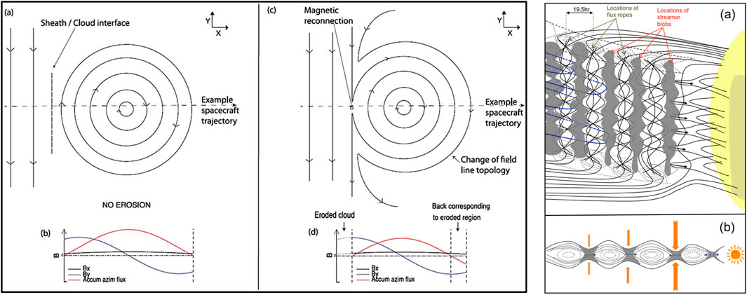
FIGURE 3. (Left) The magnetic structure of a MC, (A) prior to, and (C) during reconnection, together with (B, D) the expected variations in the magnetic field components and accumulated azimuthal magnetic flux. Image Courtesy of Ruffenach et al. (2012). (Right) Sketch of magnetic reconnection as the origin of blobs in a plane (A) containing, and (B) perpendicular to the neutral line. The gray shading denotes the high-density regions (or plasma blobs). The black lines represent the magnetic field lines around the HCS. The magnetic field lines of the flux ropes are represented with dashed black lines. The orange and blue arrows show the reconnection inflow and outflow regions, respectively. Image Courtesy of Sanchez-Diaz et al. (2017a).
1.4 Small- and meso-scale solar wind structures
Small- and meso-scale structures, such as density blobs and flux ropes, exist in the solar wind (Sanchez-Diaz et al., 2017a; Sanchez-Diaz et al., 2017b; Sanchez-Diaz et al., 2019) with scales ranging between 5 and 10,000 Mm (equivalent to transit times of 10 seconds-7 hours) and periodicities of 1–20 h (Allen et al., 2022). The meso-scale structures are released periodically from the tip of helmet streamers (periodicity of 10–20 h; Sheeley et al., 2009; Rouillard et al., 2010b). Smaller density and magnetic structures are also often observed (periodicity on the order of 1–3 h; Viall et al., 2010; Viall & Vourlidas, 2015) in the solar wind. The latter category also involves small flux ropes, as observed by Parker Solar Probe (PSP), with durations ranging between 1 and 4 h (corresponding to a size of 3 solar radii; Kepko et al., 2016).
The heliospheric current sheet (HCS) is a narrow plasma layer that divides the heliosphere into regions of opposite magnetic field polarity. In-situ observations of the HCS crossing (Winterhalter et al., 1994; Zhou et al., 2005) indicate a very thin (0.1–1.0 Earth radii in the interplanetary medium). Instead of passing through zero (change in polarity), the magnetic field rotates (that is, changes its orientation), inside the HCS (Smith et al., 2001; 2008). Magnetic reconnection is also frequently observed within the HCS (Gosling J. T. et al., 2006).
Heliospheric plasma sheet (HPS) is a high-density region, made up of a large reconnection exhaust mostly disconnected from the Sun (Lavraud et al., 2020). HPS is composed of a succession of high-β blobs and flux ropes, as shown in Figure 3, Right). The flux ropes, likely released through sequential magnetic reconnection above the helmet streamers, range in scale between tens of minutes to few tens of hours. Well-separated probes are needed to determine the structural characteristics and drivers of these different scales and periodicities, as well as their evolution and geo-effectiveness, and to derive their association to magnetic reconnection.
Turbulence is a universal process driving the transport of mass, momentum, and energy in plasmas throughout our Solar System and the Universe. Helioswarm (Spence, 2019) aims to investigate turbulence in the weakly-collisional environment of the Earth’s magnetosphere and solar wind, using an array of probes with inter-spacecraft separations ranging from fluid scales (1,000’s of km) to sub-ion kinetic scales (10s of km). Using the SWIFT measurements along the Sun-Earth line, the radial evolution of solar wind turbulence properties, ranging between 10s to 100s of RE (104 km–106 km) can be further discovered.
1.5 Space weather
Knowledge of the structure and evolution of solar wind structures are critical for reliable space weather prediction. While the magnetic cloud of an ICME forms in the solar corona, the sheath region, characterized as having enhanced thermal pressure, accumulates only during the propagation. Presently, the orientation and strength of the interplanetary magnetic field (IMF) and thermal pressure, key parameters driving space weather geo-effectiveness (Akhavan-Tafti et al., 2020), are largely unknown until the ICME has propagated to 1 AU, unless an interplanetary spacecraft with magnetic field instrument is fortuitously in the right place at the right time. Similarly, the arrival at Earth of an interplanetary shock and its accompanying energetic particle intensity enhancements (e.g., Vandegriff et al., 2005) can be forewarned by using a spacecraft conveniently located upstream of Earth (at sub-L1), capable of transmitting near-real time space weather data back to Earth. A radially aligned set of SWIFT-class probes are critical for space weather readiness, enabling doubling the current forecasting lead-times from L1.
2 Mission overview
2.1 Science traceability matrix (STM)
Space Weather Investigation Frontier (SWIFT) aims (science objective) to determine whether local or global processes drive geo-effective solar wind structures, using solar sail technology that, for the first time, will make consistent, in-situ multi-point observations along the Sun-Earth line beyond the Lagrange point L1 (sub-L1; ∼1.8-L1).
To achieve this, three main science questions are introduced. As Table 1 shows, the science questions are organized based on the general form of the energy equation for charged species (Akhavan-Tafti et al., 2019): 1) spatial terms (𝝏/𝝏x), 2) temporal terms (𝝏/𝝏t), and 3) the kinetic energy term (dU/dt).
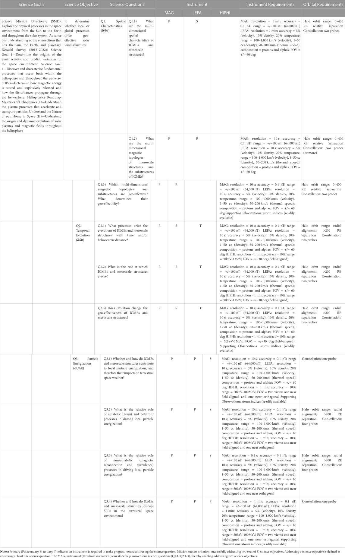
TABLE 1. SWIFT science traceability matrix.
2.1.1 Science questions
2.1.1.1 Spatial characteristics (𝝏/𝝏x)
Our current understanding of the ICME structure is based mostly on single-point or remote measurements. The ICME structures can be further complicated by the interaction of fast and slow ICMEs along their propagation paths in interplanetary space. The interaction of fast and slow ICMEs can result in many different types of complex structures, including complex jets (Gopalswamy et al., 2001; Burlaga et al., 2002; Shen et al., 2012; Lugaz et al., 2017) multi-magnetic clouds (Wang et al., 2003), and a shock-ICME structure, wherein an ICME shock transmits into a preceding ICME (Lugaz et al., 2015).
Because of a long-lasting intense southward magnetic field component (-Bz) (Tsurutani et al., 1988; Kamide et al., 1998), ICMEs can cause major geomagnetic storms (Gonzalez et al., 1994; Zhang et al., 2007; Shen et al., 2017). The geo-effectiveness of complex ICME structures, such as in a shock-ICME structure, are thought to be more significant than typical ICMEs, especially where the magnetic field intensity in the interaction structures is enhanced (Shen et al., 2017; 2018; Srivastava et al., 2018; Scolini et al., 2020). At scales smaller than ICMEs, the spatial characteristics, magnetic topologies, and geo-effectiveness of small- and meso-scale structures in the solar wind, such as density blobs and flux ropes, remain unknown.
Q1. Spatial Characteristics (𝝏/𝝏x): SWIFT will aim to answer questions regarding the multi-dimensional spatial characteristics, magnetic topologies, and geo-effectiveness of ICMEs and mesoscale structures:
Q1. 1) What are the multi-dimensional spatial characteristics of ICMEs and meso-scale structures?
Q1. 2) What are the multi-dimensional magnetic topologies of meso-scale structures and the substructures of ICMEs?
Q1. 3) Which multi-dimensional magnetic topologies and sub-structures are geo-effective? What determines their geo-effectivity?To answer these questions, at least a magnetic field instrument and a low-energy plasma instrument are needed, boarded on more than one probe, separated between 0 and 400 Earth radii, RE, perpendicular to the flow direction. The required separation will resolve small to meso-scale structures (Allen et al., 2022), as well as the substructure of large structures, such as ICMEs (Lugaz et al., 2018; Ala-Lahti et al., 2020; 2021).
2.1.1.2 Temporal evolution (𝝏/𝝏t)
The magnetic elasticity, helicity, and compression of interacting CMEs are key physical factors for determining their formation, propagation, evolution, and resultant geoeffectiveness (Xiong et al., 2006a; Xiong et al., 2006b; Xiong et al., 2007; Xiong et al., 2009). In cases where the expansion and propagation of ICME ejecta are super-magnetosonic speeds relative to the background plasma (Siscoe and Odstrcil, 2008), shock waves are particularly expected to form (Gopalswamy et al., 2010). In the corona, strong CMEs are associated with rather-explosive particle acceleration, within mere minutes after their initiation (Gopalswamy et al., 2012). In contrary, in the interplanetary medium, there are, on average, more ICMEs with shocks at 1 AU than at 0.7 AU, based on analyses of long-term observations obtained during different solar cycles (Jian et al., 2008a; Jian et al., 2008b). Furthermore, ICME sheath regions are highly variable and often very geo-effective, due to large negative Bz and/or turbulence (Huttunen and Koskinen, 2004; Kilpua et al., 2013; Katus et al., 2015; Kilpua et al., 2020). It is unknown how fast these sheaths evolve.
It is still unclear whether small- and meso-scale structures in the solar wind evolve upon generation. Large scale flux ropes, such as the magnetic cloud of an ICME, expand and relax while propagating radially away from the Sun, it is expected that small- and meso-scale structures in the solar wind to interact with each other as well as their surrounding environments, resulting in complex geo-effective characteristics (Ala-Lahti et al., 2020; 2021).
Q2. Temporal Evolution (𝝏/𝝏t): SWIFT will aim to answer questions regarding the temporal and radial evolutions of ICMEs and mesoscale structures:
Q2.1) What processes drive the evolution of ICMEs and mesoscale structures with time and/or heliocentric distance?
Q2.2) What is the rate at which ICMEs and mesoscale structures evolve?
Q2.3) Does evolution change the geo-effectiveness of ICMEs and mesoscale structures?
Answering the above questions, including the evolution of Bz associated with various solar wind structures, will require magnetic field measurements, labeled as primary (P). In this case, having a low-energy plasma instrument will enable additional science, though not required. Two or more probes are needed to answer the science questions. The probes will need to be separated radially by at least 200 RE, enabling studying the evolution of solar wind structures within a span of about 60 min.
2.1.1.3 Particle energization (dU/dt)
Solar energetic particles (SEPs) can be divided into two categories: a) impulsive, and b) gradual events (Cane et al., 1986). Impulsive events are relatively short-lived. They are typically associated with impulsive hard and soft X-ray flares, but not necessarily with large ejections of coronal material. On average, an impulsive SEP event lasts for a few hours, following the onset. These events are characterized as being rich in electron content. The 3He/4He ratio of impulsive SEP events is of the order of one, sometimes even larger than 10. In contrast, the gradual events are observable for days. Up to 96% of gradual SEP events are found to be associated with CMEs (Kahler et al., 1984). They are proton-rich, with very small 3He/4He ratio, compared to the impulsive SEP events.
The effects of small- and meso-scale solar wind structures on SEP populations are still unknown. The impulsive SEPs are thought to be accelerated close to the Sun by the rapid energy release in association with the impulsive phase of a solar flare and by the consequent strong wave activity (non-adiabatic). The non-adiabatic energization of plasmas is typically linked to processes such as magnetic reconnection and wave/turbulence interactions. By contrast, gradual SEP particles are likely driven by adiabatic energization mechanisms. The adiabatic energization of plasmas requires the conservation of the first and second adiabatic invariants, as fast CMEs expand while propagating anti-sunward.
The erosion rate of a magnetic cloud can vary at different solar wind conditions (at different solar radii). The distribution function of magnetic fluctuations in the boundary layer is significantly different from those in the ambient solar wind and the cloud body itself (Wei et al., 2003). The ICME sheath substructure may also contribute to particle energization (e.g., Kilpua et al., 2021).
The arrival of interplanetary shocks driven by ICMEs at 1 AU is not always accompanied by energetic particle intensity enhancements (e.g., Lario et al., 2003). Nevertheless, the most intense high-energy particle enhancements seen in association with shocks tend to occur when the nearby medium through which shocks propagate is affected by the presence of other solar wind structures (Lario et al., 2003). Simultaneous measurements of the magnetic field and solar wind properties are needed to characterize interplanetary shocks, the environment where these shocks propagate, and the particle populations accelerated by the shocks and the accompanying structures.
Q3. Particle Energization (dU/dt): SWIFT will aim to answer questions regarding the energization mechanisms in ICMEs and mesoscale structures:
Q3.1) Whether and how do ICMEs and mesoscale structures contribute to local particle energization, and therefore determine their impacts on terrestrial space weather?
Q3.2) What is the relative role of adiabatic (Fermi and betatron) processes in driving local particle energization?
Q3.3) What is the relative role of non-adiabatic (magnetic reconnection and turbulence) processes in driving local particle energization?
Q3.4) Whether and how do ICMEs and mesoscale structures disrupt SEPs in the terrestrial space environment?
Three of the four science questions require both magnetic field and low-energy plasma suites. The fourth science question further requires an onboard high-energy plasma detector. One probe is sufficient to answer the first and fourth questions, though four probes are needed to provide three-dimensional measurements to reliably answer the second and third questions.
2.2 Mission requirements
SWIFT aims to determine whether local or global processes generate or drive geo-effective solar wind structures. To achieve this, SWIFT will uniquely investigate the spatial (𝝏/𝝏x), temporal (𝝏/𝝏t), and total (d/dt) distributions of solar wind magnetic fields and plasmas at altitudes greater than the Earth’s Lagrange point L1. To reach this unique vantage point, SWIFT will take advantage of state-of-the-art solar sail propulsion to provide near-indefinite maneuvering and monitoring capabilities. These capabilities have been and remain unattainable by any other propulsion systems in service.
2.2.1 Instrumentation
The magnetic field instrument (threshold) can alone help answer four science questions (Q1.1, Q2.1-3), thereby addressing two science objectives (mission success criterion).
2.2.1.1 Magnetic field
The magnetic field instrument (MAG) on SWIFT will be a dual redundant digital fluxgate magnetometer consisting of two triaxial fluxgate sensors. The two sensors allow the ambient field to be separated from magnetic disturbances created by the spacecraft. This requires 1) the spacecraft to be magnetically clean, and 2) the sensors to be mounted on a rigid boom. The two sensors will be mounted at different distances from the spacecraft on the boom, hence operating as a gradiometer and thus enabling the background spacecraft magnetic field to be accurately subtracted from the measurements. MAG will cover a range of −128 to +128 nT, with time cadence of 1 s.
2.2.1.2 Low-energy ions
The low-energy proton and alpha instrument (LEPA) on SWIFT will measure the three-dimensional (3D) ion velocity distribution functions and moments (velocity, density and temperature). To achieve this, a sensor head will need to comprise a deflection unit to selectively steer and measure ions, a top-hat electrostatic analyzer, and micro-channel plates board with anodes. Arriving solar wind ions enter the instrument through an outer aperture grid. LEPA will cover a range of 50 eV to 40 keV with a 1-min (up to 10 s) resolution.
2.2.1.3 High-energy ions
The high-energy proton and heavy-ion instrument (HIPHI) consists of two oppositely-pointing field of views (FOVs): (anti-)parallel and perpendicular to the nominal Parker spiral angle. HIPHI measures protons of a lower energy threshold of 20 keV and higher energy threshold of 105 MeV. The instrument is further capable of stopping and detecting heavy ions up to 210 MeV/nuc (species dependent). HIPHI will have a resolution of 1-min (up to 6 s).
2.2.2 Solar sail technology
Solar sails are large, mirror-like structures made of a lightweight material that reflects sunlight to propel spacecraft. The source of thrust is the continuous solar photon pressure, therefore avoiding the heavy, expendable propellants used by conventional chemical and electric propulsion systems. Solar sail technology has made major advancements over the past 2 decades through Earth orbital and interplanetary flight projects. Figure 4 summarizes the various technology demonstration missions, as well as conceptual studies and ground test programs., providing a foundation for a new era of missions to utilize solar sailing to achieve space science goals (e.g., Harra et al., 2021).
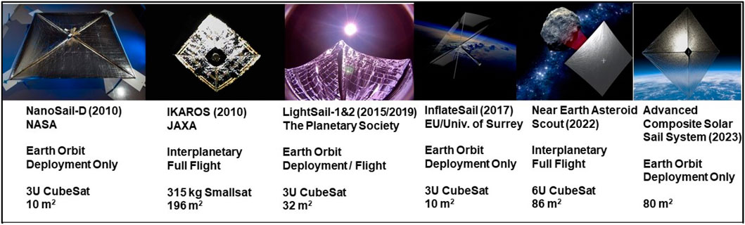
FIGURE 4. Solar sail heritage, technology readiness level (TRL), and specifications.
The Japanese Interplanetary Kite-craft Accelerated by Radiation of the Sun (IKAROS; Tsuda et al., 2013) was the first successful interplanetary solar power sail technology demonstration mission. Launched in 2022, the NASA Near-Earth Asteroid (NEA) Scout utilized an 86 m2 square solar sail to propel the 6-unit CubeSat bus on a reconnaissance flyby trajectory of asteroid 2020 GE. NEA Scout, managed by NASA Marshall Space Flight Center (MSFC), was the first space science mission designed to utilize solar sailing to achieve its science objective(s).
Solar Cruiser (Pezent et al., 2021) aims to demonstrate a 1,653 m2 sailcraft platform with pointing control and attitude stability suitable for heliophysics instruments. The mission is designed to demonstrate sailcraft operation (acceleration, navigation, station keeping, heliocentric plane change) as well as the scalability of sail technologies such as the boom, membrane, and deployer to enable more demanding missions. The sailcraft is designed to separate from the launch vehicle on a sub-L1 trajectory (1.8 L1) and complete its primary mission in 11 months. As of this writing, Solar Cruiser is not confirmed for flight. A full-scale quadrant deployment of the sail was tested (TRL = 5+) in October.
To date, solar sailing is the only viable propulsion system to allow affordable and long-term operations at the desired sub-L1 orbit. SWIFT will take advantage of a Solar Cruiser-derived solar sail propulsion system to achieve a characteristic acceleration of >0.13 mm/s2 to achieve its desired orbit.
2.2.3 Constellation configurations
Figure 5 summarizes three different constellation configurations enabling SWIFT to investigate multi-dimensional structure and dynamics of ICMEs.
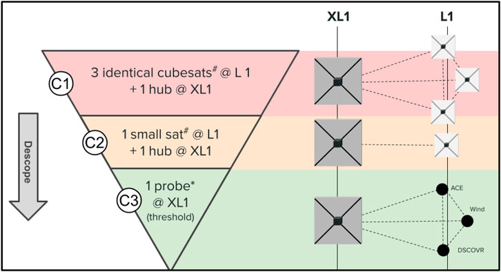
FIGURE 5. SWIFT constellation configurations. (#) sailcraft is optional for the L1 probes. (*) at least one L1 probe (ACE, WIND, DISCOVR, NASA IMAP, and NOAA SWFO) is required for the threshold configuration.
2.2.3.1 The 3:1 spoke-hub probe network
In order to independently measure the required spatial and temporal variations of solar wind structures, SWIFT will consist of four probes: one “hub,” and three “spoke” probes. The hub probe is capable of communicating with the spoke probes and transferring data to and from Earth. The spoke probes are equipped with science data collection and communication with the hub probe. The hub probe is equipped with a solar sail enabling reaching and orbiting beyond L1 (sub-L1; XL1). The spoke probes will be stationed at L1. The four probes will fly in a tetrahedron configuration, providing 3D measurements of the solar wind structures and dynamics, including gradients in magnetic field and plasma moments, similar to NASA’s flagship Magnetospheric Multiscale (MMS) mission.
2.2.3.2 The 1:1 spoke-hub probe network
Alternatively, SWIFT can independently measure the required spatial and temporal variations of solar wind structures and dynamics with the deployment of one hub probe reaching sub-L1 altitudes and one spoke probe stationed at L1. This configuration will provide 1D measurements of the solar wind structures and dynamics, including radial investigation of the magnetic field and plasma moments of solar wind structures. In this configuration, the hub probe at sub-L1, in conjunction with the L1 satellites, will further provide the required spatial and temporal variations of solar wind structures and dynamics.
2.2.3.3 Threshold configuration
SWIFT can also fly to sub-L1 altitudes as a single-probe satellite, equipped with a solar sail and scientific suites of magnetic field and plasma instruments. In this configuration, SWIFT, in conjunction with the L1 and near-Earth satellites, will provide the required spatial and temporal variations of solar wind structures and dynamics.
L1 (ACE, DSCOVR, and Wind) and near-Earth probes (MMS) can fortuitously be used to investigate the 3D characteristics of an ICME structure and its dynamics. Figure 6 shows an ICME sheath observation on 20 April 2020. MMS1 (15 RE) traversed across both the ICME shock and sheath regions. Here, the curlometer technique (Harvey, 1998) is applied on the tetrahedra of 1) L1 and MMS1 (green), and 2) MMS1-4 (black) probes to determine current density. Panels b and c show that the current densities between the two tetrahedra agree and the error is relatively small (ratio <5), respectively, indicating that the curlometer technique is reliable. SWIFT will, for the first time, enable the continuous, in-situ investigation of earthbound ICMEs’ multi-dimensional structures and dynamics.
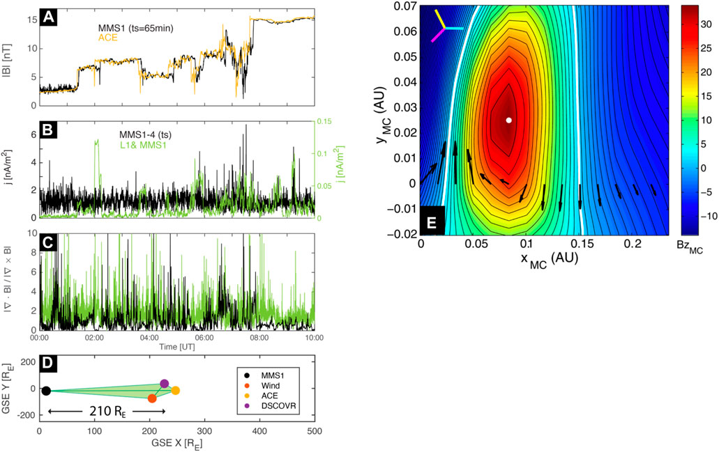
FIGURE 6. The ICME sheath of 20 April 2020. (A) Magnetic field magnitude |B| from ACE (yellow) and time-shifted (ts = 65min) MMS1 (black), (B) Current density, and (C) error, determined using the curlometer technique for MMS1-4 (black), as well as between the L1 satellites and MMS1 (green). The resolution is 10s, (D) The shape of the tetrahedron (height = 210 RE) during the multi-mission observations. (E) Reconstructed magnetic field map for ACE for an ICME observed on 9 November 2004. Image courtesy of Isavnin et al. (2011).
2.2.4 Orbital maneuvers
2.2.4.1 Stationed at sub-L1
By adding a solar sail to a spacecraft in the multi-body gravitational regime, the equilibrium liberation points are artificially shifted. In the Sun-Earth system, this shift results in a sailcraft having Lagrange point orbits that are closer to the Sun than what conventional spacecraft could achieve. Preliminary analysis, as summarized in Figure 7, shows a possible shift of around 750,000 km (∼1.8 L1) closer to the Sun. Once stationed in a sub-L1 orbit, a sailcraft can easily maneuver to other families and orbit amplitudes in the sub-L1 region to collect scientific measurements from a wide range of positions.
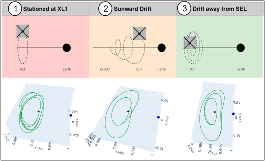
FIGURE 7. SWIFT orbital maneuvers. Sun is to the left. Earth (L1) is marked with blue (black) circle, and trajectory as green arcs.
2.2.4.2 Drifting sunward
With a “Hub” spacecraft stationed at a sail-induced sub-L1 orbit, it could be possible to maneuver the sailcraft to temporarily drift even closer to the Sun than what its sub-L1 orbit naturally does. This sunward drifting maneuver would be performed by leveraging prescribed sail pointing to perform a sail-enabled homoclinic connection to the initial sub-L1 orbit. Preliminary analysis on this maneuver suggests a shift closer to the Sun of around 250,000 km on top of the shift already gained by adding a solar sail.
2.2.4.3 Drifting away from the Sun-Earth line
To further enhance SWIFT’s ability to map the spatial characteristics of an ICME, it is possible for the “hub” spacecraft to perform a sail-enabled maneuver that drifts away from the Sun-Earth line (SEL). Similar to the sunward drift maneuver, this maneuver would utilize sail pointing angles that send the spacecraft along a prescribed path. The destination of this maneuver would be to the Lyapunov family of sub-L1 liberation point orbits, where the sailcraft can reside for as long as desired and then can transfer back to the nominal sub-L1 orbit.
2.3 Science closure
SWIFT at a vantage point of sub-L1 will enable multi-point investigations of the solar wind to distinguish temporal and spatial variations. The juxtaposition of in-situ measurements of solar wind structures and the corresponding magnetospheric response will further enable SWIFT to identify geo-effective solar wind structures. SWIFT can also enable the multi-dimensional investigation of ICMEs and meso-scale solar wind structures, essential for investigating the relative roles of local (adiabatic and non-adiabatic processes) and global (taking place in the solar corona) mechanisms in energizing solar wind plasma. Together, these studies will discover whether local or global processes drive different geo-effective solar wind structures.
2.4 Mission context
The Sentinels element (Szabo, 2005) laid the groundwork for future heliospheric missions. Their goal was to develop “the scientific understanding necessary to effectively address aspects of the Sun-Earth system that directly affect life and society.” The Sentinels envisioned an array of in-situ spacecraft monitoring solar wind characteristics at several heliocentric distances, and solar longitudes and latitudes, together with remote sensing probes. To that end, SWIFT uniquely joins a long list of heliospheric mission concepts, including Lagrange (ESA), Magnetic Topology Reconstruction Explorer (MagneToRE; Maruca et al., 2021), Polar investigation of the Sun (Polaris; Appourchaux et al., 2009; Probst et al., 2022), SPORT (Xiong et al., 2017), Solar Ring (Wang et al., 2023), and InterMeso (Allen et al., 2022) aiming to fill the observational gaps to determine the structure and long-term variations of the inner heliosphere.
3 Summary
SWIFT will aim at making major discoveries on the three-dimensional structure and dynamics of heliospheric structures that drive space weather. The spatial characteristics and temporal evolution of ICMEs are not yet well understood, and the existing remote-sensing and in situ observatories are not well-suited for resolving multi-layered and evolutionary structures in massive storm drivers. Here, we lay out the preliminary design for a groundbreaking mission using solar sail technology that, for the first time, will make consistent, in situ multi-point observations along the Sun-Earth line beyond the Lagrange point L1 (sub-L1). This unique position, in combination with L1 assets and physical models, will allow distinguishing between local and global processes, spatial characteristics, temporal evolution, and particle energization mechanisms related to ICMEs. In addition, measurements of the magnetic field in earthbound ICMEs and their sub-structures from the SWIFT location will double the current forecasting lead-times from L1.
Data availability statement
The original contributions presented in the study are included in the article/supplementary material, further inquiries can be directed to the corresponding author.
Author contributions
MA-T led the investigation, and the co-authors contributed to literature search, traceability study, and manuscript preparation. All authors contributed to the article and approved the submitted version.
Funding
This material is based upon work supported by the National Aeronautics and Space Administration (NASA) under Grant No. 80NSSC23K0674 issued through the Heliophysics Flight Opportunities Studies (HFOS) program under the Research Opportunities in Space and Earth Sciences (ROSES 2022).
Conflict of interest
The authors declare that the research was conducted in the absence of any commercial or financial relationships that could be construed as a potential conflict of interest.
Publisher’s note
All claims expressed in this article are solely those of the authors and do not necessarily represent those of their affiliated organizations, or those of the publisher, the editors and the reviewers. Any product that may be evaluated in this article, or claim that may be made by its manufacturer, is not guaranteed or endorsed by the publisher.
References
Akhavan-Tafti, M., Fontaine, D., Slavin, J. A., Le Contel, O., and Turner, D. (2020). Cross-scale quantification of storm-time dayside magnetospheric magnetic flux content. J. Geophys. Res. Space Phys.125 (10), e2020JA028027. doi:10.1029/2020ja028027
Akhavan-Tafti, M., Slavin, J. A., Sun, W. J., Le, G., and Gershman, D. J. (2019). MMS observations of plasma heating associated with FTE growth. Geophys. Res. Lett.46 (22), 12654–12664. doi:10.1029/2019gl084843
Ala-Lahti, M., Dimmock, A. P., Pulkkinen, T. I., Good, S. W., Yordanova, E., Turc, L., et al. (2021). Transmission of an ICME sheath into the Earth's magnetosheath and the occurrence of traveling foreshocks. J. Geophys. Res. Space Phys.126 (12), e2021JA029896. doi:10.1029/2021ja029896
Ala-Lahti, M., Ruohotie, J., Good, S., Kilpua, E. K., and Lugaz, N. (2020). Spatial coherence of interplanetary coronal mass ejection sheaths at 1 AU. J. Geophys. Res. Space Phys.125 (9), e2020JA028002. doi:10.1029/2020ja028002
Allen, R., Smith, E., Anderson, B., Borovsky, J., Ho, G., Xu, J., et al. (2022). Interplanetary mesoscale observatory (InterMeso): A mission to untangle dynamic mesoscale structures throughout the heliosphere. Front. Astronomy Space Sci.9. doi:10.3389/fspas.2022.1002273
Appourchaux, T., Liewer, P., Watt, M., Alexander, D., Andretta, V., Auchère, F., et al. (2009). POLAR investigation of the Sun—polaris. Exp. Astron.23, 1079–1117. doi:10.1007/s10686-008-9107-8
Burch, J. L., Torbert, R. B., Phan, T. D., Chen, L. J., Moore, T. E., Ergun, R. E., et al. (2016). Electron-scale measurements of magnetic reconnection in space. Science352 (6290), aaf2939. doi:10.1126/science.aaf2939
Burlaga, L. F., Plunkett, S. P., and Cyr, St.O. C. (2002). Successive CMEs and complex ejecta. J. Geophys. Res. Space Phys.107 (A10), SSH–1. doi:10.1029/2001JA000255
Burlaga, L. F., Sittler, E., Mariani, F., and Schwenn, R. (1981). Magnetic loop behind an interplanetary shock: Voyager, Helios and IMP-8 observations. J. Geophys. Res.86, 6673. doi:10.1029/ja086ia08p06673
Cane, H. V., McGuire, R. V., and Von Rosenvinge, T. T. (1986). Two classes of solar energetic particle events associated with impulsive and long-duration soft X-ray flares. Astrophysical J.301, 448–459. doi:10.1086/163913
Davies, E. E., Möstl, C., Owens, M. J., Weiss, A. J., Amerstorfer, T., Hinterreiter, J., et al. (2021). In situ multi-spacecraft and remote imaging observations of the first CME detected by Solar Orbiter and BepiColombo. Astronomy Astrophysics656, A2. doi:10.1051/0004-6361/202040113
Davies, J. A., Harrison, R. A., Perry, C. H., Möstl, C., Lugaz, N., Rollett, T, et al. (2012). A self-similar expansion model for use in solar wind transient propagation studies. Astrophysical J.750 (1), 23. doi:10.1088/0004-637x/750/1/23
Davis, M. S., Phan, T. D., Gosling, J. T., and Skoug, R. M. (2006). Detection of oppositely directed reconnection jets in a solar wind current sheet. Geophys. Res. Lett.33 (19), L19102. doi:10.1029/2006gl026735
DeForest, C. E., Howard, T. A., and Tappin, S. J. (2011). Observations of detailed structure in the solar wind at 1 AU with STEREO/HI-2. Astrophysical J.738 (1), 103. doi:10.1088/0004-637x/738/1/103
Eriksson, S., Gosling, J. T., Phan, T. D., Blush, L. M., Simunac, K. D. C., Krauss-Varban, D., et al. (2009). Asymmetric shear flow effects on magnetic field configuration within oppositely directed solar wind reconnection exhausts. J. Geophys. Res. Space Phys.114 (A7). doi:10.1029/2008ja013990
Farrugia, C. J., Gratton, F. T., and Torbert, R. B. (2001). Viscous-type processes in the solar wind-magnetosphere interaction. Space Sci. Rev.95 (1), 443–456. doi:10.1023/a:1005288703357
Fenrich, F. R., and Luhmann, J. G. (1998). Geomagnetic response to magnetic clouds of different polarity. Geophys. Res. Lett.25 (15), 2999–3002. doi:10.1029/98gl51180
Fermo, R. L., Opher, M., and Drake, J. F. (2014). Magnetic reconnection in the interior of interplanetary coronal mass ejections. Phys. Rev. Lett.113 (3), 031101. doi:10.1103/physrevlett.113.031101
Gonzalez, W. D., Joselyn, J. A., Kamide, Y., Kroehl, H. W., Rostoker, G., Tsurutani, B. T., et al. (1994). What is a geomagnetic storm?J. Geophys. Res. Space Phys.99 (A4), 5771–5792. doi:10.1029/93ja02867
Gonzalez, W. D., and Tsurutani, B. T. (1987). Criteria of interplanetary parameters causing intense magnetic storms (Dst<− 100 nT). Planet. Space Sci.35 (9), 1101–1109. doi:10.1016/0032-0633(87)90015-8
Gopalswamy, N., Xie, H., Mäkelä, P., Akiyama, S., Yashiro, S., Kaiser, M. L., et al. (2010). Interplanetary shocks lacking type II radio bursts. Astrophysical J.710 (2), 1111–1126. doi:10.1088/0004-637x/710/2/1111
Gopalswamy, N., Xie, H., Yashiro, S., Akiyama, S., Mäkelä, P., and Usoskin, I. G. (2012). Properties of ground level enhancement events and the associated solar eruptions during solar cycle 23. Space Sci. Rev.171 (1), 23–60. doi:10.1007/s11214-012-9890-4
Gopalswamy, N., Yashiro, S., Kaiser, M. L., Howard, R. A., and Bougeret, J. L. (2001). Radio signatures of coronal mass ejection interaction: Coronal mass ejection cannibalism?Astrophysical J.548 (1), L91–L94. doi:10.1086/318939
Gosling, J. T. (1990). in Geophys. Monogr. Ser. 58 Editors C. T. Russell, E. R. Priest, and L. C. Lee (Washington: AGU), 343.
Gosling, J. T., Eriksson, S., Skoug, R. M., McComas, D. J., and Forsyth, R. J. (2006b). Petschek-type reconnection exhausts in the solar wind well beyond 1 AU: Ulysses. Astrophysical J.644 (1), 613–621. doi:10.1086/503544
Gosling, J. T., McComas, D. J., Skoug, R. M., and Smith, C. W. (2006a). Magnetic reconnection at the heliospheric current sheet and the formation of closed magnetic field lines in the solar wind. Geophys. Res. Lett.33 (17), L17102. doi:10.1029/2006gl027188
Gosling, J. T., Skoug, R. M., McComas, D. J., and Smith, C. W. (2005). Direct evidence for magnetic reconnection in the solar wind near 1 AU. J. Geophys. Res. Space Phys.110 (A1), A01107. doi:10.1029/2004ja010809
Gosling, J. T., and Szabo, A. (2008). Bifurcated current sheets produced by magnetic reconnection in the solar wind. J. Geophys. Res. Space Phys.113 (A10). doi:10.1029/2008ja013473
Harra, L., Andretta, V., Appourchaux, T., Baudin, F., Bellot-Rubio, L., Birch, A. C., et al. (2021). A journey of exploration to the polar regions of a star: Probing the solar poles and the heliosphere from high helio-latitude. Exp. Astron.54, 157–183. doi:10.1007/s10686-021-09769-x
Harrison, R. A., Davis, C. J., Eyles, C. J., Bewsher, D., Crothers, S. R., Davies, J. A., et al. (2008). First imaging of coronal mass ejections in the heliosphere viewed from outside the Sun–Earth line. Sol. Phys.247, 171–193. doi:10.1007/s11207-007-9083-6
Harvey, C. C. (1998). Spatial gradients and the volumetric tensor. In G. Paschmann, and P. W. Daly (Eds.) Analysis methods for multi-spacecraft data, ISSI Scientific Reports SR-001. (Washington: International Space Science Institute), 07–322.
Huttunen, K. E. J., Bale, S. D., and Salem, C. (2008). Wind observations of low energy particles within a solar wind reconnection region. Ann. Geophys.26, 2701–2710. doi:10.5194/angeo-26-2701-2008
Huttunen, K. E. J., and Koskinen, H. E. J. (2004). Importance of post-shock streams and sheath region as drivers of intense magnetospheric storms and high-latitude activity. Ann. Geophys.22 (5), 1729–1738. doi:10.5194/angeo-22-1729-2004
Isavnin, A., Kilpua, E. K., and Koskinen, H. E. (2011). Grad–shafranov reconstruction of magnetic clouds: Overview and improvements. Sol. Phys.273 (1), 205–219. doi:10.1007/s11207-011-9845-z
Jian, L. K., Russell, C. T., Luhmann, J. G., Skoug, R. M., and Steinberg, J. (2008b). Stream interactions and interplanetary coronal mass ejections at 0.72 AU. Sol. Phys.249 (1), 85–101. doi:10.1007/s11207-008-9161-4
Jian, L. K., Russell, C. T., Luhmann, J. G., Skoug, R. M., and Steinberg, J. T. (2008a). Stream interactions and interplanetary coronal mass ejections at 5.3 AU near the solar ecliptic plane. Sol. Phys.250 (2), 375–402. doi:10.1007/s11207-008-9204-x
Kahler, S. W., Sheeley, N. R., Howard, R. A., Koomen, M. J., Michels, D. J., McGuire, R. V., et al. (1984). Associations between coronal mass ejections and solar energetic proton events. J. Geophys. Res. Space Phys.89 (A11), 9683–9693. doi:10.1029/ja089ia11p09683
Kamide, Y., Yokoyama, N., Gonzalez, W., Tsurutani, B. T., Daglis, I. A., Brekke, A., et al. (1998). Two-step development of geomagnetic storms. J. Geophys. Res. Space Phys.103 (A4), 6917–6921. doi:10.1029/97ja03337
Katus, R. M., Liemohn, M. W., Ionides, E. L., Ilie, R., Welling, D., and Sarno-Smith, L. K. (2015). Statistical analysis of the geomagnetic response to different solar wind drivers and the dependence on storm intensity. J. Geophys. Res. Space Phys.120 (1), 310–327. doi:10.1002/2014ja020712
Kepko, L., Viall, N. M., Antiochos, S. K., Lepri, S. T., Kasper, J. C., and Weberg, M. (2016). Implications of L1 observations for slow solar wind formation by solar reconnection. Geophys. Res. Lett.43 (9), 4089–4097. doi:10.1002/2016gl068607
Kilpua, E. K., Fontaine, D., Good, S. W., Ala-Lahti, M., Osmane, A., Palmerio, E., et al. (2020). Magnetic field fluctuation properties of coronal mass ejection-driven sheath regions in the near-Earth solar wind. Ann. Geophys.38 (5), 999–1017. doi:10.5194/angeo-38-999-2020
Kilpua, E. K. J., Good, S. W., Dresing, N., Vainio, R., Davies, E. E., Forsyth, R. J., et al. (2021). Multi-spacecraft observations of the structure of the sheath of an interplanetary coronal mass ejection and related energetic ion enhancement. Astronomy Astrophysics656, A8. doi:10.1051/0004-6361/202140838
Kilpua, E. K. J., Hietala, H., Koskinen, H. E. J., Fontaine, D., and Turc, L. (2013). Magnetic field and dynamic pressure ULF fluctuations in coronal-mass-ejection-driven sheath regions. Ann. Geophys.31 (9), 1559–1567. doi:10.5194/angeo-31-1559-2013
Klein, L. W., and Burlaga, L. F. (1982). Interplanetary magnetic clouds at 1 AU. J. Geophys. Res.87, 613. doi:10.1029/ja087ia02p00613
Lario, D., Ho, G. C., Decker, R. B., Roelof, E. C., Desai, M. I., and Smith, C. W. (2003). ACE observations of energetic particles associated with transient interplanetary shocks. AIP Conf. Proc.679 (No. 1), 640–643. doi:10.1063/1.1618676
Lavraud, B., Fargette, N., Réville, V., Szabo, A., Huang, J., Rouillard, A. P., et al. (2020). The heliospheric current sheet and plasma sheet during Parker Solar Probe’s first orbit. Astrophysical J. Lett.894 (2), L19. doi:10.3847/2041-8213/ab8d2d
Lavraud, B., Gosling, J. T., Rouillard, A. P., Fedorov, A., Opitz, A., Sauvaud, J. A., et al. (2009). Observation of a complex solar wind reconnection exhaust from spacecraft separated by over 1800 RE. Sol. Phys.256 (1), 379–392. doi:10.1007/s11207-009-9341-x
Lavraud, B., Ruffenach, A., Rouillard, A. P., Kajdic, P., Manchester, W. B., and Lugaz, N. (2014). Geo-effectiveness and radial dependence of magnetic cloud erosion by magnetic reconnection. J. Geophys. Res. Space Phys.119 (1), 26–35. doi:10.1002/2013ja019154
Lepping, R. P., Jones, J. A., and Burlaga, L. F. (1990). Magnetic field structure of interplanetary magnetic clouds at 1 AU. J. Geophys. Res. Space Phys.95 (A8), 11957–11965. doi:10.1029/ja095ia08p11957
Lugaz, N., Farrugia, C. J., Smith, C. W., and Paulson, K. (2015). Shocks inside CMEs: A survey of properties from 1997 to 2006. J. Geophys. Res. Space Phys.120 (4), 2409–2427. doi:10.1002/2014ja020848
Lugaz, N., Farrugia, C. J., Winslow, R. M., Al-Haddad, N., Galvin, A. B., Nieves-Chinchilla, T., et al. (2018). On the spatial coherence of magnetic ejecta: Measurements of coronal mass ejections by multiple spacecraft longitudinally separated by 0.01 au. Astrophysical J. Lett.864 (1), L7. doi:10.3847/2041-8213/aad9f4
Lugaz, N., Temmer, M., Wang, Y., and Farrugia, C. J. (2017). The interaction of successive coronal mass ejections: A review. Sol. Phys.292, 64–37. doi:10.1007/s11207-017-1091-6
Marubashi, K. (1986). Structure of the interplanetary magnetic clouds and their solar origins. Adv. Space Res.6, 335–338. doi:10.1016/0273-1177(86)90172-9
Maruca, B. A., Agudelo Rueda, J. A., Bandyopadhyay, R., Bianco, F. B., Chasapis, A., Chhiber, R, et al. (2021). MagneToRE: Mapping the 3-D magnetic structure of the solar wind using a large constellation of nanosatellites. Front. Astronomy Space Sci.8, 665885. doi:10.3389/fspas.2021.665885
Möstl, C., Rollett, T., Temmer, M., Farrugia, C. J., Veronig, A., Galvin, A. B., et al. (2010). Direction and orientation of CME/ICME events observed by STEREO. 38th COSPAR Sci. Assem.38, 8. https://ui.adsabs.harvard.edu/abs/2010cosp.38.1881M/abstract
Nieves-Chinchilla, T., Alzate, N., Cremades, H., Rodríguez-García, L., Dos Santos, L. F., Narock, A., et al. (2022). Direct first parker solar probe observation of the interaction of two successive interplanetary coronal mass ejections in 2020 november. Astrophysical J.930 (1), 88. doi:10.3847/1538-4357/ac590b
Owens, M. J., Démoulin, P., Savani, N. P., Lavraud, B., and Ruffenach, A. (2012). Implications of non-cylindrical flux ropes for magnetic cloud reconstruction techniques and the interpretation of double flux rope events. Sol. Phys.278, 435–446. doi:10.1007/s11207-012-9939-2
Pezent, J. B., Sood, R., Heaton, A., Miller, K., and Johnson, L. (2021). Preliminary trajectory design for NASA’s solar cruiser: A technology demonstration mission. Acta Astronaut.183, 134–140. doi:10.1016/j.actaastro.2021.03.006
Phan, T. D., Gosling, J. T., Davis, M. S., Skoug, R. M., Øieroset, M., Lin, R. P., et al. (2006). A magnetic reconnection X-line extending more than 390 Earth radii in the solar wind. Nature439 (7073), 175–178. doi:10.1038/nature04393
Probst, A., Anderson, T., Farrish, A. O., Kjellstrand, C. B., Newheart, A. M., Thaller, S. A., et al. (2022). Sun sailing polar orbiting telescope (SunSPOT): A solar polar imaging mission design. Adv. Space Res.70, 510–522. doi:10.1016/j.asr.2022.04.060
Rouillard, A. P., Davies, J. A., Lavraud, B., Forsyth, R. J., Savani, N. P., Bewsher, D., et al. (2010a). Intermittent release of transients in the slow solar wind: 1. Remote sensing observations. J. Geophys. Res. Space Phys.115 (A4). doi:10.1029/2009ja014471
Rouillard, A. P., Lavraud, B., Sheeley, N. R., Davies, J. A., Burlaga, L. F., Savani, N. P., et al. (2010b). White light and in situ comparison of a forming merged interaction region. Astrophysical J.719 (2), 1385–1392. doi:10.1088/0004-637x/719/2/1385
Ruffenach, A., Lavraud, B., Owens, M. J., Sauvaud, J. A., Savani, N. P., Rouillard, A. P., et al. (2012). Multispacecraft observation of magnetic cloud erosion by magnetic reconnection during propagation. J. Geophys. Res. Space Phys.117 (A9). doi:10.1029/2012ja017624
Russell, C. T., Wang, Y. L., Raeder, J., Tokar, R. L., Smith, C. W., Ogilvie, K. W., et al. (2000). The interplanetary shock of september 24, 1998: Arrival at earth. J. Geophys. Res.105, 25143–25154. doi:10.1029/2000ja900070
Sanchez-Diaz, E., Rouillard, A. P., Davies, J. A., Lavraud, B., Pinto, R. F., and Kilpua, E. (2017b). The temporal and spatial scales of density structures released in the slow solar wind during solar activity maximum. Astrophysical J.851 (1), 32. doi:10.3847/1538-4357/aa98e2
Sanchez-Diaz, E., Rouillard, A. P., Davies, J. A., Lavraud, B., Sheeley, N. R., Pinto, R. F., et al. (2017a). Observational evidence for the associated formation of blobs and raining inflows in the solar corona. Astrophysical J. Lett.835 (1), L7. doi:10.3847/2041-8213/835/1/l7
Sanchez-Diaz, E., Rouillard, A. P., Lavraud, B., Kilpua, E., and Davies, J. A. (2019). In situ measurements of the variable slow solar wind near sector boundaries. Astrophysical J.882 (1), 51. doi:10.3847/1538-4357/ab341c
Schrijver, C. J., Kauristie, K., Aylward, A. D., Denardini, C. M., Gibson, S. E., Glover, A., et al. (2015). Understanding space weather to shield society: A global road map for 2015–2025 commissioned by cospar and ilws. Adv. Space Res.55 (12), 2745–2807. doi:10.1016/j.asr.2015.03.023
Scolini, C., Chané, E., Temmer, M., Kilpua, E. K., Dissauer, K., Veronig, A. M., et al. (2020). CME–CME interactions as sources of CME geoeffectiveness: The formation of the complex ejecta and intense geomagnetic storm in 2017 early September. Astrophysical J. Suppl. Ser.247 (1), 21. doi:10.3847/1538-4365/ab6216
Sheeley, N. R., Lee, D. H., Casto, K. P., Wang, Y. M., and Rich, N. B. (2009). The structure of streamer blobs. Astrophysical J.694 (2), 1471–1480. doi:10.1088/0004-637x/694/2/1471
Shen, C., Chi, Y., Wang, Y., Xu, M., and Wang, S. (2017). Statistical comparison of the ICME's geoeffectiveness of different types and different solar phases from 1995 to 2014. J. Geophys. Res. Space Phys.122 (6), 5931–5948. doi:10.1002/2016ja023768
Shen, C., Xu, M., Wang, Y., Chi, Y., and Luo, B. (2018). Why the shock-ICME complex structure is important: Learning from the early 2017 september CMEs. Astrophysical J.861 (1), 28. doi:10.3847/1538-4357/aac204
Shen, F., Wu, S. T., Feng, X., and Wu, C. C. (2012). Acceleration and deceleration of coronal mass ejections during propagation and interaction. J. Geophys. Res. Space Phys.117 (A11). doi:10.1029/2012ja017776
Siscoe, G., and Odstrcil, D. (2008). Ways in which ICME sheaths differ from magnetosheaths. J. Geophys. Res. Space Phys.113 (A9). doi:10.1029/2008ja013142
Smith, E. J.2008, in The heliosphere through the solar activity cycle, ed. A. Balogh, L. J. Lanzerotti, and S. T. Suess, Springer Praxis Books (Berlin, Heidelberg: Springer), 79
Smith, E. J., Balogh, A., Forsyth, R. J., and McComas, D. J. (2001). Ulysses in the south polar cap at solar maximum: Heliospheric magnetic field. Geophys. Res. Lett.28, 4159–4162. doi:10.1029/2001gl013471
Spence, H. E. (2019). HelioSwarm: Unlocking the multiscale mysteries of weakly-collisional magnetized plasma turbulence and ion heating. AGU Fall Meet. Abstr.2019, SH11B–04. https://ui.adsabs.harvard.edu/abs/2019AGUFMSH11B.04S/abstract
Srivastava, N., Mishra, W., and Chakrabarty, D. (2018). Interplanetary and geomagnetic consequences of interacting CMEs of 13–14 June 2012. Sol. Phys.293 (1), 5–12. doi:10.1007/s11207-017-1227-8
Szabo, A. (2005). The living with a star (LWS) Sentinels. Adv. Space Res.35 (1), 61–64. doi:10.1016/j.asr.2004.09.013
Tsuda, Y., Mori, O., Funase, R., Sawada, H., Yamamoto, T., Saiki, T., et al. (2013). Achievement of IKAROS—Japanese deep space solar sail demonstration mission. Acta Astronaut.82 (2), 183–188. doi:10.1016/j.actaastro.2012.03.032
Tsurutani, B. T., Gonzalez, W. D., Tang, F., Akasofu, S. I., and Smith, E. J. (1988). Origin of interplanetary southward magnetic fields responsible for major magnetic storms near solar maximum (1978–1979). J. Geophys. Res. Space Phys.93 (A8), 8519–8531. doi:10.1029/ja093ia08p08519
Vandegriff, J., Wagstaff, K., Ho, G., and Plauger, J. (2005). Forecasting space weather: Predicting interplanetary shocks using neural networks. Adv. Space Res.36 (12), 2323–2327. doi:10.1016/j.asr.2004.09.022
Viall, N. M., Spence, H. E., Vourlidas, A., and Howard, R. (2010). Examining periodic solar-wind density structures observed in the SECCHI heliospheric imagers. Sol. Phys.267 (1), 175–202. doi:10.1007/s11207-010-9633-1
Viall, N. M., and Vourlidas, A. (2015). Periodic density structures and the origin of the slow solar wind. Astrophysical J.807 (2), 176. doi:10.1088/0004-637x/807/2/176
Wang, Y., Bai, X., Chen, C., Chen, L., Cheng, X., Deng, L., et al. (2023). Solar ring mission: Building a panorama of the Sun and inner-heliosphere. Adv. Space Res.71 (1), 1146–1164. doi:10.1016/j.asr.2022.10.045
Wang, Y. M., Ye, P. Z., and Wang, S. (2003). Multiple magnetic clouds: Several examples during march–april 2001. J. Geophys. Res. Space Phys.108 (A10), 1370. doi:10.1029/2003ja009850
Webb, D. F., and Howard, T. A. (2012). Coronal mass ejections: Observations. Living Rev. Sol. Phys.9 (1), 1–83. doi:10.12942/lrsp-2012-3
Wei, F., Liu, R., Fan, Q., and Feng, X. (2003). Identification of the magnetic cloud boundary layers. J. Geophys. Res. Space Phys.108 (A6), 1263. doi:10.1029/2002ja009511
Weiss, A. J., Möstl, C., Amerstorfer, T., Bailey, R. L., Reiss, M. A., Hinterreiter, J., et al. (2021a). Analysis of coronal mass ejection flux rope signatures using 3DCORE and approximate bayesian computation. ApJS252, 9. doi:10.3847/1538-4365/abc9bd
Wilson, R. M. (1987). Geomagnetic response to magnetic clouds. Planet. space Sci.35 (3), 329–335. doi:10.1016/0032-0633(87)90159-0
Winterhalter, D., Smith, E. J., Burton, M. E., Murphy, N., and McComas, D. (1994). The heliospheric plasma sheet. JGR99, 6667. doi:10.1029/93ja03481
Xiong, M., Davies, J. A., Li, B., Yang, L., Liu, Y. D., Xia, L., et al. (2017). Prospective out-of-ecliptic white-light imaging of interplanetary corotating interaction regions at solar maximum. Astrophysical J.844 (1), 76. doi:10.3847/1538-4357/aa7aaa
Xiong, M., Zheng, H., and Wang, S. (2009). Magnetohydrodynamic simulation of the interaction between two interplanetary magnetic clouds and its consequent geoeffectiveness: 2. Oblique collision. J. Geophys. Res. Space Phys.114 (A11). doi:10.1029/2009ja014079
Xiong, M., Zheng, H., Wang, Y., and Wang, S. (2006b). Magnetohydrodynamic simulation of the interaction between interplanetary strong shock and magnetic cloud and its consequent geoeffectiveness. J. Geophys. Res. Space Phys.111 (A8), A08105. doi:10.1029/2005ja011593
Xiong, M., Zheng, H., Wang, Y., and Wang, S. (2006a). Magnetohydrodynamic simulation of the interaction between interplanetary strong shock and magnetic cloud and its consequent geoeffectiveness: 2. Oblique collision. J. Geophys. Res. Space Phys.111 (A11), A11102. doi:10.1029/2006ja011901
Xiong, M., Zheng, H., Wu, S. T., Wang, Y., and Wang, S. (2007). Magnetohydrodynamic simulation of the interaction between two interplanetary magnetic clouds and its consequent geoeffectiveness. J. Geophys. Res. Space Phys.112 (A11). doi:10.1029/2007ja012320
Zhang, J., Richardson, I. G., Webb, D. F., Gopalswamy, N., Huttunen, E., Kasper, J. C., et al. (2007). Solar and interplanetary sources of major geomagnetic storms (Dst≤− 100 nT) during 1996–2005. J. Geophys. Res. Space Phys.112 (A10). doi:10.1029/2007ja012321
Zhou, X.-Y., Smith, E. J., and Winterhalter, D. (2005). in Proceedings of solar wind 11-SOHO 16, connecting Sun and heliosphere, whistler, Canada 12–17 june.
Keywords: space weather, interplanetary coronal mass ejection (ICME), geomagnetic storm, solar sail propulsion, mesoscale solar wind structures, sub-L1
Citation: Akhavan-Tafti M, Johnson L, Sood R, Slavin JA, Pulkkinen T, Lepri S, Kilpua E, Fontaine D, Szabo A, Wilson L, Le G, Atilaw TY, Ala-Lahti M, Soni SL, Biesecker D, Jian LK and Lario D (2023) Space weather investigation Frontier (SWIFT). Front. Astron. Space Sci. 10:1185603. doi: 10.3389/fspas.2023.1185603
Received: 13 March 2023; Accepted: 09 June 2023;
Published: 29 June 2023.
Edited by:
Vladislav Izmodenov, Space Research Institute (RAS), RussiaReviewed by:
Elena Provornikova, Johns Hopkins University, United StatesXueshang Feng, Chinese Academy of Sciences (CAS), China
Copyright © 2023 Akhavan-Tafti, Johnson, Sood, Slavin, Pulkkinen, Lepri, Kilpua, Fontaine, Szabo, Wilson, Le, Atilaw, Ala-Lahti, Soni, Biesecker, Jian and Lario. This is an open-access article distributed under the terms of the Creative Commons Attribution License (CC BY). The use, distribution or reproduction in other forums is permitted, provided the original author(s) and the copyright owner(s) are credited and that the original publication in this journal is cited, in accordance with accepted academic practice. No use, distribution or reproduction is permitted which does not comply with these terms.
*Correspondence: M. Akhavan-Tafti, YWtoYXZhbnRAdW1pY2guZWR1