 Solène Lejosne
 Jay M. Albert
- 1Space Sciences Laboratory, University of California, Berkeley, Berkeley, CA, United States
- 2Air Force Research Laboratory, Kirtland AFB, Albuquerque, NM, United States
Most physics-based models provide a coarse three-dimensional representation of radiation belt dynamics at low time resolution, of the order of a few drift periods. The description of the effect of trapped particle transport on radiation belt intensity is based on the random phase approximation, and it is in one dimension only: the third adiabatic invariant coordinate, akin to a phase-averaged radial distance. This means that these radiation belt models do not resolve the drift phase or, equivalently, the magnetic local time. Yet, in situ measurements suggest that radiation belt intensity frequently depends on magnetic local time, at least transiently, such as during active times. To include processes generating azimuthal variations in trapped particle fluxes and to quantify their relative importance in radiation belt energization, an improvement in the spatiotemporal resolution of the radiation belt models is required. The objective of this study is to pave the way for a new generation of diffusive radiation belt models capable of retaining drift phase information. Specifically, we highlight a two-dimensional equation for the effects of trapped particle transport on radiation belt intensity. With a theoretical framework that goes beyond the radial diffusion paradigm, the effects of trapped particle bulk motion, as well as diffusion, are quantified in terms of Euler potentials,
1 Introduction
The motion of energetic particles trapped in planetary radiation belts is a superposition of three quasi-periodic motions, each evolving on a very distinct spatiotemporal scale, with an amplitude quantified by an adiabatic invariant (e.g., Northrop and Teller, 1960; Schulz and Lanzerotti, 1974):
(1) A very fast and small motion of gyration around the magnetic field direction.
(2) A slower and bigger bounce motion between the planet’s hemispheres, along the magnetic field direction.
(3) A slow and large drift motion around the planet in a direction perpendicular to the magnetic field direction.
The scale separation between these three quasi-periodic motions spans several orders of magnitude in time and space.
Combining adiabatic invariant theory with Fokker–Planck formalism yields the theoretical framework for a probabilistic model of radiation belt dynamics (e.g., Roederer and Zhang, 2014). The Fokker–Planck formalism accounts for uncertainties in electromagnetic field characterization. The adiabatic theory allows for a three-dimensional phase-averaged representation of radiation belt dynamics rather than a full six-dimensional description in phase space.
The description of radiation belt dynamics as a three-dimensional Fokker–Planck equation reduced to a diffusion equation requires minimal computational resources. This quality has enabled the development of many radiation belt computer codes over the years: Salammbô (e.g., Beutier and Boscher, 1995; Nénon et al., 2017), Diffusion in (I,L,B) Energetic Radiation Tracker (DILBERT) (Albert et al., 2009), Versatile Electron Radiation Belt (VERB) (Subbotin and Shprits, 2009), Storm-Time Evolution of Electron Radiation Belt (STEERB) (Su et al., 2010), DREAM3D, as part of the Dynamic Radiation Environment Assimilation Model (DREAM) project (Tu et al., 2013), and British Antarctic Survey Radiation Belt Model (BAS RBM) (Glauert et al., 2014; Woodfield et al., 2014) are all examples of radiation belt codes relying on the same theoretical basis. While first implemented in the case of terrestrial radiation belts, the three-dimensional Fokker–Planck equation has also been transposed to the radiation belts of Jupiter and Saturn. The resulting codes are widely used for scientific research (e.g., Varotsou et al., 2005; Woodfield et al., 2018; Drozdov et al., 2020) and for space weather purposes (e.g., Glauert et al., 2018; Horne et al., 2021).
On the technical side, these computer codes consist of solving a diffusion equation that provides an approximate description for the time evolution of the radiation belts:
where
From a theoretical standpoint, it is a reasonable first approximation to consider that radiation belt intensity is independent of magnetic local time: any
In all cases, processes generating drift-periodic signatures are important due to their connection to radiation belt energization (e.g., Hudson et al., 2020). Yet, three-dimensional radiation belt models cannot account for the generation of drift-periodic signatures. Instead, drift-periodic signatures are usually modeled independently of other processes, by tracking the drift motion of test particles (guiding centers) in prescribed electric and magnetic fields, omitting local processes occurring along the gyration and bounce motions (such as local acceleration by chorus waves for instance) (e.g., Li et al., 1993; Hudson et al., 2017).
In that context, it is necessary to introduce a general equation for radiation belt dynamics that includes
Since this work focuses on improving the modeling of drift effects on radiation belt intensity, we first assume conservation of the first two adiabatic invariants. Thus, all considered quantities are bounce-averaged. We also omit any significant source or loss mechanism. A generalization of the resulting transport equation to include diffusion of the first two adiabatic invariants is straightforward. It is provided at the end of Section 3.
2 Theoretical background
We briefly recall how to derive the standard radial diffusion equation. This informs how to derive the same equation as the one proposed by Birmingham et al. (1967) (Section 3). We also detail the concept of Euler potentials and highlight their connection to the third adiabatic invariant.
2.1 Derivation of the standard radiation belt radial diffusion equation
In the following section, the third adiabatic invariant,
where
which can also be written as
To transform this equation into a radial diffusion equation, we use the fact that the two coefficients
(e.g., Lichtenberg and Lieberman, 1992, their section 5.4a; Lejosne and Kollmann, 2020, their section 2.3.2). This relationship (Eq. 5) relies on the assumption of drift phase homogeneity, also known as random drift phase approximation, meaning that each drift phase location is equiprobable. In this context, the Fokker–Planck Eq. 2 reduces to a diffusion equation:
where
where
2.2 Euler potentials
An appropriate coordinate to discuss radial diffusion is the
2.2.1 Third adiabatic invariant, deconstructed in terms of Euler potentials
The radial diffusion equation, retrieved in Section 2.1 (Eq. 7), describes the time evolution of the number of particles per unit of third adiabatic invariant,
where
An important underlying requirement to sort trapped particle fluxes using the third adiabatic invariant is the so-called frozen field condition, where in the presence of magnetic field time variations, the cold (frozen) plasma
The Euler potentials
Thus, the Euler potentials are constant along the magnetic field lines. Since the vector potential can be viewed as
Although there is no uniformity in the definition of the Euler potentials, a suitable set of Euler potentials in a magnetic dipole field is
where
In the presence of a distorted magnetic field, the expressions provided in Eq. 11 are not valid anymore. That said, it is possible to leverage the facts that (a) the field line footpoints are rooted at ionospheric altitudes, a region where the ambient magnetic field is mainly dipolar, so the Euler potentials can be described by Eq. 11 at ionospheric altitudes and (b) the Euler potentials are constant along the magnetic field lines. With that in mind, we can define a set of Euler potentials
where (
If a distorted magnetic field were to change into a dipole field, each field line would “move” in geospace, adopting a dipolar shape, while its footpoints would stay rooted at fixed ionospheric latitudes. Leveraging Eq. 11 in the newly transformed dipole field, a dipolar field line with footpoints at (
The physical interpretation of this thought experiment is similar to the physical interpretation of the
where
Combining Eqs 10, 15, given that
The parameter
An illustration to the concepts discussed here is provided in Figure 1.
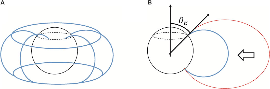
FIGURE 1. (A) A few magnetic field lines constitutive of a trapped particle drift shell, together with the locations of the field line footpoints, necessary to determine the L* parameter—adapted from Roederer (1970). (B) A stretch magnetic field line (in red) is relaxed into its dipolar shape (in blue). The field line footpoint remains rooted at the same ionospheric colatitude,
2.2.2 Euler potentials as appropriate variables to describe bounce-average drift motion of trapped and quasi-trapped particles
The Euler potentials
where
where
One consequence of Eq. 17 is that the variations of the Euler potentials are related:
This property will be leveraged to transform a two-dimensional Fokker–Planck equation in terms of Euler potentials,
3 New derivation of Birmingham et al.’s transport equation to describe trapped particle transport effects on radiation belt intensity
Here, we present a compact way to retrieve the equation proposed by Birmingham et al. (1967). This equation represents the time evolution of radiation belt intensity due to transport processes. We describe the time evolution of a distribution function,
where the angle bracket sign,
The terms between the large parentheses in Eq. 21 are
and
Using the Hamiltonian relationships between the Euler potentials (Eq. 17), we have shown in the Appendix that
provided that the time interval,
Combining Eqs 21–24, Eq. 20 becomes a drift-diffusion equation:
Given Eq. 19, this simplifies to
where
The term depending on
The transport parameters of Eq. 27 are all statistically averaged quantities. The coefficients
That is, it is half the time rate of change of the ensemble average for the product of the time variations of X and Y during a time interval,
According to Eq. 26, variations in the distribution function are due to the bulk motion of the plasma in the presence of density gradients and to diffusive effects in both the localized radial (
where all quantities are bounce-averaged quantities that depend on the drift phase.
4 Conclusion
The objective of this work is to contribute toward improving the spatiotemporal resolution of physics-based diffusive radiation belt models. The resulting transport Eq. 27 can resolve the drift phase, and the outputs are bounce-averaged rather than drift-averaged. This is of use when the objective is to model fast radiation belt dynamics, such as times of fast radiation belt acceleration or losses occurring during the main phase of geomagnetic storms (e.g., Ripoll et al., 2020; Lejosne et al., 2022). It can also be used to increase the energy range modeled, by including ring current energies.
Although Eq. 27 contains some localized (in
Current works leveraging in situ measurements to quantify radial diffusion coefficients require information on average over all magnetic local times of a drift shell. Yet, a spacecraft can only scan the electromagnetic environment along its orbit, limiting the accuracy with which the outputs can be determined (e.g., Sandhu et al., 2021). Because the coefficients introduced in this work depend on magnetic local time, these may be easier to quantify experimentally. Furthermore, describing the effect of drift motion on radiation belt intensity in terms of Euler potentials, or similarly with (
The second part of this work will deal with characterizing the coefficients introduced in Eq. 27 (i.e.,
Data availability statement
The original contributions presented in the study are included in the article/Supplementary Material, further inquiries can be directed to the corresponding author.
Author contributions
We describe contributions to the paper using the CRediT (Contributor Roles Taxonomy) categories (Brand et al., 2015). Conceptualization, writing—original draft, and writing—review and editing: all authors. Visualization: SL. All authors contributed to the article and approved the submitted version.
Acknowledgments
SL’s work was performed under NASA Grants 80NSSC18K1223 and 80NSSC20K1351. The author thanks S.D. Walton for helpful comments on a draft version of this manuscript.
Conflict of interest
The authors declare that the research was conducted in the absence of any commercial or financial relationships that could be construed as a potential conflict of interest.
Publisher’s note
All claims expressed in this article are solely those of the authors and do not necessarily represent those of their affiliated organizations, or those of the publisher, the editors, and the reviewers. Any product that may be evaluated in this article, or claim that may be made by its manufacturer, is not guaranteed or endorsed by the publisher.
References
Albert, J. M., Meredith, N. P., and Horne, R. B. (2009). Three-dimensional diffusion simulation of outer radiation belt electrons during the 9 October 1990 magnetic storm. J. Geophys. Res.114, A09214. doi:10.1029/2009JA014336
Beutier, T., and Boscher, D. (1995). A three-dimensional analysis of the electron radiation belt by the Salammbô code. J. Geophys. Res.100 (8), 14853–14861. doi:10.1029/94JA03066
Birmingham, T. J., and Jones, F. C. (1968). Identification of moving magnetic field lines. J. Geophys. Res.73 (17), 5505–5510. doi:10.1029/JA073i017p05505
Birmingham, T. J., Northrop, T. G., and Fälthammar, C. G. (1967). Charged particle diffusion by violation of the third adiabatic invariant. Phys. Fluids10 (11), 2389. doi:10.1063/1.1762048
Bourdarie, S., Boscher, D., Beutier, T., Sauvaud, J.-A., and Blanc, M. (1997). Electron and proton radiation belt dynamic simulations during storm periods: A new asymmetric convection-diffusion model. J. Geophys. Res.102 (8), 17541–17552. doi:10.1029/97JA01305
Brand, A., Allen, L., Altman, M., Hlava, M., and Scott, J. (2015). Beyond authorship: Attribution, contribution, collaboration, and credit. Learn. Pub.28, 151–155. doi:10.1087/20150211
Drozdov, A. Y., Usanova, M. E., Hudson, M. K., Allison, H. J., and Shprits, Y. Y. (2020). The role of hiss, chorus, and EMIC waves in the modeling of the dynamics of the multi-MeV radiation belt electrons. J. Geophys. Res. Space Phys.125, e2020JA028282. doi:10.1029/2020JA028282
Fälthammar, C.-G., and Mozer, F. S. (2007). [Comment on “Bringing space physics concepts into introductory electromagnetism”] on the concept of moving magnetic fields lines. Eos Trans. AGU88, 169–170. doi:10.1029/2007EO150002
Fok, M.-C., Buzulukova, N. Y., Chen, S.-H., Glocer, A., Nagai, T., Valek, P., et al. (2014). The comprehensive inner magnetosphere-ionosphere model. J. Geophys. Res. Space Phys.119, 7522–7540. doi:10.1002/2014JA020239
Fok, M. C., and Moore, T. E. (1997). Ring current modeling in a realistic magnetic field configuration. J. Geophys. Res.24 (14), 1775–1778. doi:10.1029/97GL01255
Glauert, S. A., Horne, R. B., and Meredith, N. P. (2018). A 30-year simulation of the outer electron radiation belt. Space weather.16, 1498–1522. doi:10.1029/2018SW001981
Glauert, S. A., Horne, R. B., and Meredith, N. P. (2014). Three-dimensional electron radiation belt simulations using the BAS Radiation Belt Model with new diffusion models for chorus, plasmaspheric hiss, and lightning-generated whistlers. J. Geophys. Res. Space Phys.119, 268–289. doi:10.1002/2013JA019281
Hao, Y. X., Sun, Y. X., Roussos, E., Liu, Y., Kollmann, P., Yuan, C. J., et al. (2020). The formation of saturn’s and jupiter’s electron radiation belts by magnetospheric electric fields. Astrophysical J.905 (1), L10. doi:10.3847/2041-8213/abca3f
Hao, Y. X., Zong, Q. G., Zhou, X. Z., Fu, S. Y., Rankin, R., Yuan, C. J., et al. (2016). Electron dropout echoes induced by interplanetary shock: Van Allen Probes observations. Geophys. Res. Lett.43, 5597–5605. doi:10.1002/2016GL069140
Horne, R. B., Glauert, S. A., Kirsch, P., Heynderickx, D., Bingham, S., Thorn, P., et al. (2021). The satellite risk prediction and radiation forecast system (SaRIF). Space weather.19, e2021SW002823. doi:10.1029/2021SW002823
Hudson, M., Jaynes, A., Kress, B. T., Li, Z., Patel, M., Shen, X.-C., et al. (2017). Simulated prompt acceleration of multi-MeV electrons by the 17March 2015 interplanetary shock. J. Geophys. Research:Space Phys.122, 10,036–10,046. doi:10.1002/2017JA024445
Hudson, M. K., Elkington, S. R., Li, Z., and Patel, M. (2020). Drift echoes and flux oscillations: A signature of prompt and diffusive changes in the radiation belts. J. Atmos. Solar-Terrestrial Phys.207, 105332. doi:10.1016/j.jastp.2020.105332
Jordanova, V. K., Kozyra, J. U., Nagy, A. F., and Khazanov, G. V. (1997). Kinetic model of the ring current-atmosphere interactions. J. Geophys. Res.102 (7), 14279–14291. doi:10.1029/96JA03699
Jordanova, V. K., Morley, S. K., Engel, M. A., Godinez, H. C., Yakymenko, K., Henderson, M. G., et al. (2022). The RAM-SCB model and its applications to advance space weather forecasting. Adv. Space Res.doi:10.1016/j.asr.2022.08.077
Lejosne, S., Allison, H. J., Blum, L. W., Drozdov, A. Y., Hartinger, M. D., Hudson, M. K., et al. (2022). Differentiating between the leading processes for electron radiation belt acceleration. Front. Astron. Space Sci.9, 896245. doi:10.3389/fspas.2022.896245
Lejosne, S. (2014). An algorithm for approximating the L * invariant coordinate from the real-time tracing of one magnetic field line between mirror points. J. Geophys. Res. Space Phys.119, 6405–6416. doi:10.1002/2014JA020016
Lejosne, S., and Kollmann, P. (2020). Radiation belt radial diffusion at Earth and beyond. Space Sci. Rev.216, 19. doi:10.1007/s11214-020-0642-6
Lejosne, S., and Mozer, F. S. (2020). Experimental determination of the conditions associated with “zebra stripe” pattern generation in the earth's inner radiation belt and slot region. J. Geophys. Res. Space Phys.125, e2020JA027889. doi:10.1029/2020JA027889
Li, X., Roth, I., Temerin, M., Wygant, J. R., Hudson, M. K., and Blake, J. B. (1993). Simulation of the prompt energization and transport of radiation belt particles during the March 24, 1991 SSC. Geophys. Res. Lett.20 (22), 2423–2426. doi:10.1029/93gl02701
Lichtenberg, A. J., and Lieberman, M. A. (1992). “Regular and chaotic dynamics,” in Applied mathematical Sciences. 2nd (New York: Springer).
Nénon, Q., Sicard, A., and Bourdarie, S. (2017). A new physical model of the electron radiation belts of Jupiter inside Europa's orbit. J. Geophys. Res. Space Phys.122, 5148–5167. doi:10.1002/2017JA023893
Northrop, T. G., and Teller, E. (1960). Stability of the adiabatic motion of charged particles in the earth's field. Phys. Rev.117 (1), 215–225. doi:10.1103/PhysRev.117.215
Patel, M., Li, Z., Hudson, M., Claudepierre, S., and Wygant, J. (2019). Simulation of prompt acceleration of radiation belt electrons during the 16 July 2017 storm. Geophys. Res. Lett.46, 7222–7229. doi:10.1029/2019GL083257
Ripoll, J.-F., Claudepierre, S. G., Ukhorskiy, A. Y., Colpitts, C., Li, X., Fennell, J., et al. (2020). Particle dynamics in the earth's radiation belts: Review of current research and open questions. J. Geophys. Res. Space Phys.125, e2019JA026735. doi:10.1029/2019JA026735
Roederer, J. G. (1967). On the adiabatic motion of energetic particles in a model magnetosphere. J. Geophys. Res.72 (3), 981–992. doi:10.1029/JZ072i003p00981
Roederer, J. G., and Zhang, H. (2014). “Dynamics of magnetically trapped particles,” in Foundations of the physics of radiation belts and space plasmas. Astrophysics and space science library (Berlin: Springer).
Sandhu, J. K., Rae, I. J., Wygant, J. R., Breneman, A. W., Tian, S., Watt, C. E. J., et al. (2021). ULF wave driven radial diffusion during geomagnetic storms: A statistical analysis of van allen probes observations. J. Geophys. Res. Space Phys.126, e2020JA029024. doi:10.1029/2020JA029024
Sauvaud, J.-A., Walt, M., Delcourt, D., Benoist, C., Penou, E., Chen, Y., et al. (2013). Inner radiation belt particle acceleration and energy structuring by drift resonance with ULF waves during geomagnetic storms. J. Geophys. Res. Space Phys.118, 1723–1736. doi:10.1002/jgra.50125
Schulz, M., and Lanzerotti, L. J. (1974). Particle diffusion in the radiation belts. Heidelberg: Springer Berlin.
Shprits, Y. Y., Kellerman, A. C., Drozdov, A. Y., Spence, H. E., Reeves, G. D., and Baker, D. N. (2015), Combined convective and diffusive simulations: VERB-4D comparison with 17 march 2013 van allen probes observations, Geophys. Res. Lett.42, 9600–9608. doi:10.1002/2015GL065230
Stern, D. (1967). Geomagnetic euler potentials. J. Geophys. Res.72 (15), 3995–4005. doi:10.1029/jz072i015p03995
Su, Z., Xiao, F., Zheng, H., and Wang, S. (2010). Steerb: A three-dimensional code for storm-time evolution of electron radiation belt. J. Geophys. Res.115, A09208. doi:10.1029/2009JA015210
Subbotin, D. A., and Shprits, Y. Y. (2009). Three-dimensional modeling of the radiation belts using the Versatile Electron Radiation Belt (VERB) code. Space weather.7, S10001. doi:10.1029/2008SW000452
Tu, W., Cunningham, G. S., Chen, Y., Henderson, M. G., Camporeale, E., and Reeves, G. D. (2013). Modeling radiation belt electron dynamics during GEM challenge intervals with the DREAM3D diffusion model. J. Geophys. Res. Space Phys.118, 6197–6211. doi:10.1002/jgra.50560
Ukhorskiy, A. Y., and Sitnov, M. I. (2013). Dynamics of radiation belt particles. Space Sci. Rev.179, 545–578. doi:10.1007/s11214-012-9938-5
Varotsou, A., Boscher, D., Bourdarie, S., Horne, R. B., Glauert, S. A., and Meredith, N. P. (2005). Simulation of the outer radiation belt electrons near geosynchronous orbit including both radial diffusion and resonant interaction with Whistler-mode chorus waves. Geophys. Res. Lett.32, L19106. doi:10.1029/2005GL023282
Walt, M. (1994). Introduction to geomagnetically trapped radiation. Cambridge: Cambridge University Press. doi:10.1017/CBO9780511524981
Woodfield, E. E., Horne, R. B., Glauert, S. A., Menietti, J. D., Shprits, Y. Y., and Kurth, W. S. (2018). Formation of electron radiation belts at Saturn by Z-mode wave acceleration. Nat. Commun.9, 5062. doi:10.1038/s41467-018-07549-4
Woodfield, E. E., Horne, R. B., Glauert, S. A., Menietti, J. D., and Shprits, Y. Y. (2014). The origin of Jupiter's outer radiation belt. J. Geophys. Res. Space Phys.119, 3490–3502. doi:10.1002/2014JA019891
Yu, Y., Jordanova, V. K., Ridley, A. J., Albert, J. M., Horne, R. B., and Jeffery, C. A. (2016). A new ionospheric electron precipitation module coupled with RAM-SCB within the geospace general circulation model. J. Geophys. Res. Space Phys.121, 8554–8575. doi:10.1002/2016JA022585
Zhao, H., Sarris, T. E., Li, X., Huckabee, I. G., Baker, D. N., Jaynes, A. J., et al. (2022). Statistics of multi-MeV electron drift-periodic flux oscillations using Van Allen Probes observations. Geophys. Res. Lett.49, e2022GL097995. doi:10.1029/2022GL097995
Glossary
Appendix
Here, we detail how to obtain Eq. 24, leveraging the fact that the Euler potentials (
We assume some small variations in
Rewriting
(see also Lichtenberg and Lieberman, 1992; their equation (5.4.10), p. 322).
Combining equations Eqs A1, A2, 17, we have
To the second order in
Thus,
Combining Eqs A3–A5 in terms of expected values for the variations, we have
Assuming that the time interval,
with
Keywords: radiation belts, Fokker–Planck equation, adiabatic invariants, Euler potentials, radial transport, radial diffusion, azimuthal diffusion
Citation: Lejosne S and Albert JM (2023) Drift phase resolved diffusive radiation belt model: 1. Theoretical framework. Front. Astron. Space Sci. 10:1200485. doi: 10.3389/fspas.2023.1200485
Received: 05 April 2023; Accepted: 08 June 2023;
Published: 04 July 2023.
Edited by:
Qianli Ma, Boston University, United StatesReviewed by:
Paul O’Brien, The Aerospace Corporation, United StatesZhenpeng Su, University of Science and Technology of China, China
Copyright © 2023 Lejosne and Albert. This is an open-access article distributed under the terms of the Creative Commons Attribution License (CC BY). The use, distribution or reproduction in other forums is permitted, provided the original author(s) and the copyright owner(s) are credited and that the original publication in this journal is cited, in accordance with accepted academic practice. No use, distribution or reproduction is permitted which does not comply with these terms.
*Correspondence: Solène Lejosne, c29sZW5lQGJlcmtlbGV5LmVkdQ==