A system science methodology develops a new composite highly predictable index of magnetospheric activity for the community: the whole-Earth index E(1)

For community use, a new composite whole-Earth index E₍₁₎ and its matching composite solar wind driving function S₍₁₎ are derived. A system science methodology is used based on a time-dependent magnetospheric state vector and a solar wind state vector, with canonical correlation analysis (CCA) used to reduce the two state vectors to the two time-dependent scalars E₍₁₎(t) and S₍₁₎(t). The whole-Earth index E₍₁₎ is based on a diversity of measures via six diverse geomagnetic indices that will be readily available in the future: SML, SMU, Ap60, SYMH, ASYM, and PCC. The CCA-derived composite index has several advantages: 1) the new “canonical” geomagnetic index E₍₁₎ will provide a more powerful description of magnetospheric activity, a description of the collective behavior of the magnetosphere–ionosphere system. 2) The new index E₍₁₎ is much more accurately predictable from upstream solar wind measurements on Earth. 3) Indications are that the new canonical geomagnetic index E₍₁₎ will be accurately predictable even when as-yet-unseen extreme solar wind conditions occur. The composite solar wind driver S₍₁₎ can also be used as a universal driver function for individual geomagnetic indices or for magnetospheric particle populations. To familiarize the use of the new index E₍₁₎, its behavior is examined in different phases of the solar cycle, in different types of solar wind plasma, during high-speed stream-driven storms, during CME sheath-driven storms, and during superstorms. It is suggested that the definition of storms are the times when E₍₁₎ >1.

1 Introduction

The objective of this paper is to develop and present a convenient, accurate, highly predictable composite geomagnetic index that can be used by the space physics community to gauge global magnetospheric activity. This project addressed a prime goal of the NSF GEM program: “The goal of the GEM program is to make accurate predictions of the geospace environment ….” Accurate predictions of individual geospace indices have been difficult; this project took an innovative approach based on system science (Borovsky and Valdivia, 2018) and developed a magnetospheric activity index E₍₁₎ that is highly predictable based on the knowledge of solar wind on Earth [e.g., a knowledge of the properties of solar wind yields a high prediction efficiency for the value of the activity index E₍₁₎], and the new activity index E₍₁₎ is useful for gauging of the magnitude of magnetospheric activity.

Magnetospheric activity occurs in reaction to the solar wind (Dungey, 1961; Axford and Hines, 1961). This activity takes a number of forms (cf. Table 4 of Borovsky and Valdivia, 2018) and is measured by a number of geomagnetic indices that are sensitive to diverse current systems (cf. Table 1): magnetospheric (and ionospheric) convection, auroral activity, cross-polar cap current, plasma diamagnetism, cross-tail current, ULF wave activity, and Pc1 activity. There are well-known correlations between geomagnetic indices and solar wind, enabling the geomagnetic indices to be predicted (to some degree) from a knowledge of upstream solar wind parameters. Two examples appear in Figure 1, where for the years 1991–2007, the 1-hr-lagged auroral electrojet index AE(t) is plotted in panel (a) as a function of the “Newell” driver function dΦ/dt = _vsw^4/3_B⊥^2/3_{sin8/3(θclock/2)} (Newell et al., 2007) and where the 1-hr-lagged Kp index is plotted in panel (b) as a function of the “quick reconnection function,” R_quick = n_sw^1/2 v_sw² sin²(θ_clock/2) M_A^−1.35 [1 + 680M_A^−3.30]^−1/4 (Borovsky and Yakymenko, 2017a), where v_sw represents the solar wind speed; n_sw represents the solar wind number density; B_⊥ represents the component of the solar wind magnetic field, which is perpendicular to the Sun–Earth line; θ_clock represents the clock angle of the solar wind magnetic field relative to the Earth’s magnetic dipole; and M_A represents the Alfven Mach number of upstream solar wind. Each point in Figure 1 represents 1 h of data. In Figure 1B, the discrete values of Kp are spread vertically in the plot to aid the eye by adding random numbers between −0.3 and +0.3. In both panels, the red line is a least-squares linear regression fit to the black points, and the blue curve is a 50-point vertical running average of the black points.

TABLE 1

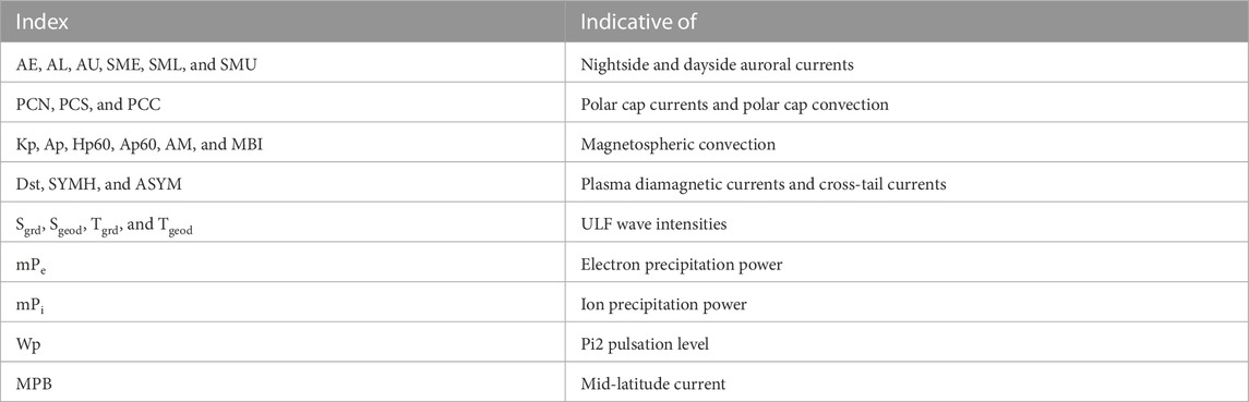
TABLE 1. Some geomagnetic indices and the processes that they respond to.

FIGURE 1

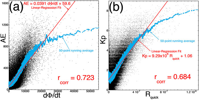
FIGURE 1. Two examples (A and B) of the correlations between a single geomagnetic index (vertical) and a common solar-wind driver function (horizontal). Each point is 1 h of data.

In Figure 1A, the Pearson linear correlation coefficient between AE(t) and the Newell dΦ/dt(t) is r_corr = 0.723. The amount of variance of AE(t) that is not described by dΦ/dt(t) is 1-r_corr² = 0.477; i.e., 47.7% of the variance of AE cannot be predicted from a knowledge of the value of dΦ/dt. As can be noticed by the local vertical spread in points in Figure 1A, there can be large errors in the value of AE, as predicted from a known value of dΦ/dt.

Single geomagnetic indices are predicted from solar wind measurements to gauge the upcoming space weather. For example, the NOAA Space Weather Prediction Center (https://www.swpc.noaa.gov) predicts the Kp index and uses it as a gauge of the strength of the activity. The IZMIRAN Space Weather Prediction Center (http://spaceweather.izmiran.ru/eng/forecasts.html) and the Parsec vzw SpaceWeatherLive (spaceweatherlive.com) also predict Kp. The British Geological Survey geomagnetic and solar activity forecast service (http://geomag.bgs.ac.uk/data_service/space_weather/forecast.html) and the Royal Observatory of Belgium Solar Influences Data Center (http://sidc.oma.be/products/meu/) both predict Ap. The University of Colorado LASP Space Weather Data (http://lasp.colorado.edu/space_weather/dsttemerin/dsttemerin.html) predicts Dst and AE. The single geomagnetic index Dst is used to gauge the intensity of storms (e.g., Sugiura and Chapman, 1960; Loewe and Prolss, 1997), as is the single geomagnetic index Kp (e.g., the NOAA SWPC Space Weather Scales). Borovsky and Sprits (2017a) have criticized the use of the single geomagnetic index Dst for gauging storm properties, in particular because one category of geomagnetic storms (high-speed stream-driven storms) occurs without producing strong Dst signatures (Borovsky and Denton, 2006).

The new composite magnetospheric activity index (Earth index) E₍₁₎ introduced in this paper will provide two, and possibly a third, improvements for magnetospheric research and space weather over the use of a single geomagnetic index. 1) The new “canonical” geomagnetic index E₍₁₎ will provide a more powerful description of magnetospheric activity: a description of the collective behavior of the magnetosphere–ionosphere system. 2) The new canonical geomagnetic index E₍₁₎ will be more accurately predictable from upstream solar wind measurements on Earth. Furthermore, 3) indications are that the new canonical geomagnetic index E₍₁₎ will be accurately predictable even when as-yet-unseen extreme solar wind conditions occur. The new magnetospheric activity index is described in Section 4.

From a systems science point of view, a “state vector” comprising several measures would provide a superior indication of the intensity of global geospace activity (Vassiliadis, 2006; Luo, 2010). In this paper, a composite scalar magnetospheric index E₍₁₎ will be derived from vector–vector correlations between a magnetospheric state vector and a solar wind state vector.

The outline of this paper is as follows: Section 2elaborates the advantages of a system-wide (whole-Earth) index. Section 3explains the canonical correlation analysis (CCA) methodology used to derive the composite Earth index E₍₁₎. Section 4provides the composite index E₍₁₎(t) created from six geomagnetic indices, along with its matching composite solar wind driver S₍₁₎(t). Section 5examines the importance of individual indices and individual solar wind variables. Section 6 examines the behavior of E₍₁₎ in different phases of the solar cycle and in different types of solar wind plasma. Section 7 uses the composite index E₍₁₎ to examine geomagnetic storms. Section 8 discusses future work needed to better understand E₍₁₎ and its driving by S₍₁₎.

2 Advantages of a system-wide (whole-Earth) index

Single geomagnetic indices can be predicted from solar wind measurements to gauge the upcoming space weather, but single geomagnetic indices tend to measure a single aspect of magnetospheric activity (cf. Table 1), and their prediction efficiency from a knowledge of solar wind on Earth is usually weak.

In developing and studying composite magnetospheric activity indices derived with the mathematical technique called canonical correlation analysis (Borovsky, 2014; Borovsky and Denton, 2014; Borovsky and Denton 2018; Borovsky and Osmane, 2019), several properties have been learned that make composite indices ideal for describing magnetospheric activity levels and the solar wind driving of the magnetosphere–ionosphere system. These advantages are enumerated in Table 2.

TABLE 2

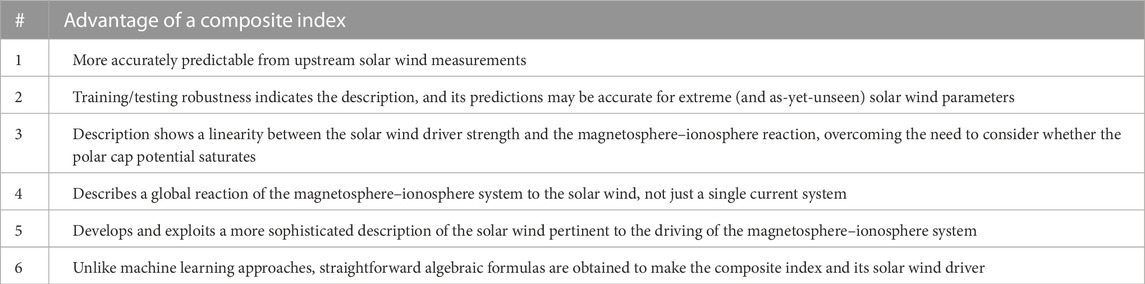
TABLE 2. Advantages of CCA-derived composite magnetospheric activity indices over single geomagnetic indices.

The first advantage listed in Table 2 (more accurately predictable) comes about for a number of reasons: 1) the composite index is describing a global mode of reaction of the magnetosphere to the solar wind with an aggregate variable (which is a weighted average of multiple variables that react to the solar wind in similar fashions), which has less noise than a single variable (a single index). 2) The methodology uses a complex solar wind description that is much more sophisticated than commonly used driver functions based on solar wind electric fields or the amount of magnetic flux delivered to the magnetosphere; composite solar wind driving can account for Mach number effects, number density effects, dipole tilt effects, B_y effects, turbulence effects, solar ionization effects, etc.

The second advantage listed in Table 2 is the robustness of the derivation of the composite index and its solar wind driver. This is an important advantage. Borovsky and Denton (2018) found that comparing derivations made on different subsets of the magnetospheric and solar wind data demonstrates the robustness of the definition of the composite activity index. For example, 1) if the composite variables are derived using only slow solar wind, the method is still very accurate for fast solar wind; 2) if the composite variables are derived using only the low-geomagnetic activity data, the method is still very accurate for high levels of activity; and 3) if the composite variables are derived using only solar-minimum data, they are still very accurate at the solar maximum. This ability to accurately predict when radically different data are presented indicates that this method may be able to predict the magnetospheric composite index accurately if very extreme, not-yet-seen solar wind parameters occur. This will be discussed in Section 7.

The third advantage listed in Table 2 is the linearity of the response of the composite geomagnetic index to the composite solar wind driver via the CCA-derived scalar functions [cf. Figure 2A of Borovsky and Denton (2018)]. This linearity means that the response of the magnetosphere–ionosphere system to solar wind is the same at strong driving (and high activity) as it is at weak driving (and low activity). This is related to the robustness found in deriving with one category of data and testing with another category (advantage 2 in Table 2). The linearity of the response eliminates the consideration of polar cap potential saturation ( Wygant et al., 1983; Reiff and Luhmann, 1986; Weimer et al., 1990; Borovsky et al., 2009; Myllys et al., 2017), which causes some individual geomagnetic indices to saturate under low-Mach number solar wind conditions (Lavraud and Borovsky, 2008; Borovsky, 2021a). The observed linearity may be interpreted as follows: if the “correct” description of magnetospheric activity is used and if the “correct” solar wind driving function is used, the reaction of the magnetosphere to solar wind driving is linear.

FIGURE 2

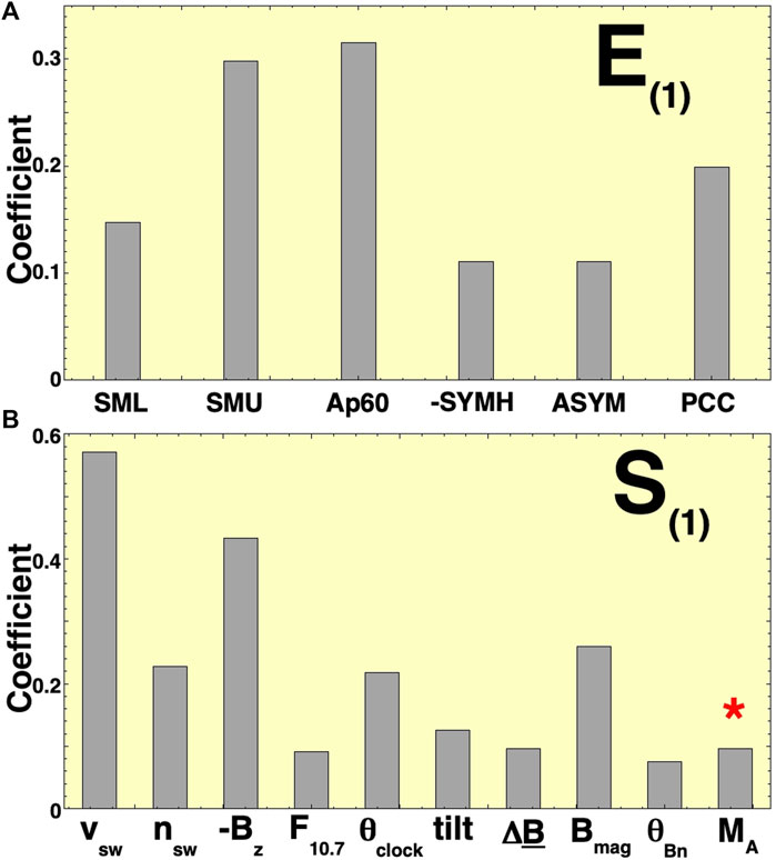
FIGURE 2. Visual representation of the coefficients of expression (1) for E₍₁₎ [panel (A)] and of the coefficients of expression (2) for S₍₁₎ [panel (B)]. The red asterisk reminds the reader that that coefficient [on the log₁₀(M_A)* term] is negative; two other negative coefficients are made positive in the graph by taking −SYMH and −B_z.

The fourth advantage listed in Table 2 is that the composite magnetospheric activity index describes a global mode of reaction of the magnetosphere–ionosphere system to solar wind. Canonical correlation analysis has so far found three independent modes of reaction of the magnetosphere–ionosphere system to solar wind (Borovsky and Osmane, 2019): the mode that will be described by the “canonical” geomagnetic index E₍₁₎ in this paper is the fundamental (first) mode, in which all measures of geomagnetic activity increase together or decrease together. Using a composite geomagnetic index instead of a single geomagnetic index is akin to describing economic activity with a stock-market index instead of a single stock.

The fifth advantage listed in Table 2 is that the processes of using CCA to develop a composite geomagnetic index also develops a much more sophisticated solar wind driver S₍₁₎ than the driver functions developed empirically (Holzer and Slavin, 1982; Newell et al., 2007; 2008; McPherron et al., 2015) or developed via physical derivations (Borovsky, 2008; 2013; Borovsky and Birn, 2014) [for extensive lists of existing driver function, see Table 1 of Newell et al., (2008) and Table 1 of Lockwood and McWilliams (2021)]. The CCA composite solar wind driver can account for Mach number effects, dipole tilt effects, B_y effects, solar ionization effects, upstream turbulence effects, etc., and S₍₁₎ can serve as a “universal driver function” with improved correlations with individual geomagnetic indices.

The sixth advantage listed in Table 2 is that two simple algebraic formulas are given, one to generate the composite magnetospheric index E₍₁₎(t) from the geomagnetic indices and the other to generate the associated solar wind driver function S₍₁₎(t) from upstream solar wind variables. Unlike machine learning methods, one does not need to run the data analysis algorithm to obtain E₍₁₎(t) and S₍₁₎(t). The algebraic formulas yield straightforward interpretations of what E₍₁₎ and S₍₁₎ are. If machine learning (e.g., neural network) algorithms were used for magnetospheric predictions, no such straightforward interpretation would be possible: one would need to run numerical experiments on the machine learning algorithm to determine how it works.

3 Methodology and data used to develop the composite index E₍₁₎ and its solar wind driver S₍₁₎

A multivariable time-dependent “Earth” dataset comprising six commonly available geomagnetic indices is used, along with a multivariable time-dependent “solar wind” dataset comprising 10 standard measurements of solar wind on Earth. The variables of each of the two datasets are listed in Table 3. One-hour averages of all quantities are used for the years 1997–2020, with 1-hr-resolution geomagnetic indices commonly available. The 10 solar wind variables were extracted from the 1-hr-resolution OMNI2 solar wind dataset (King and Papitashvili, 2005), with no time lags between the solar wind on Earth (OMNI2) and the geomagnetic indices (time lags in the CCA analysis between the solar wind and the magnetosphere were studied in Borovsky (2020a) and were found to have little effect). The geomagnetic indices in Table 3 should be mostly familiar. SYMH is very similar to Dst. SML and SMU are SuperMAG (Gjerloev et al., 2012) improvements to the AL and AU auroral electrojet indices. Ap60 is a 60-minute-resolution version of the Ap index. The PCC index is a combination of the PCI-north and PCI-south indices (Stauning, 2021). Standard values for the indices are used where SML, SMU, SYMH, and ASYM are in units of nT; PCC is in units of mV/m, and Ap60 is dimensionless. The solar wind variables in Table 3 should also be mostly familiar; the solar wind flow speed is represented by v_sw (in km/s), n_sw (in cm⁻³) represents the solar wind number density, B_z3 (in nT) represents the GSM Z component of the solar wind magnetic field, B_mag (in nT) represents the magnetic field strength in the solar wind, and F_10.7 (in 10^–22 W m⁻² Hz_-1) represents the 10.7-cm radio flux from the Sun; the tilt (in degrees) is the Sunward tilt of the Earth’s northern magnetic pole, going from −34.8^o to +34.8^o, which governs the angle at which the solar wind hits the dayside magnetosphere and relates to the amount of hinging of the cross-tail current sheet. The dipole tilt angle can be calculated using Eq. 3 of Nowada et al. (2009). The variable θ_Bn (in degrees) represents the angle between the solar wind magnetic field line and the Sun–Earth axis, going from 0^o (radial field) to 90^o. The angle θ_clock (in degrees) represents the (GSM) clock angle θ_clock = arccos(B_z/(B_y²+B_z²)^1/2). ΔB represents the rms amplitude of the vectormagnetic field fluctuations in the upstream solar wind during each hour of the OMNI2 dataset, measured typically at L1. Finally, M_A (dimensionless) is the Alfven Mach number of the upstream solar wind given by M_A = B_mag/(4πm_in_sw)^1/2. Three of the solar wind variables in Table 3 (with subscript “3”) are 3-h averages into the past, involving the present hour and two previous hours: the CCA process is significantly improved when these two 3-h averages are implemented. Most of the solar wind variables used here have appeared in “standard” solar wind driver functions (cf. Table 1 of Newell et al., 2008 or Table 1 of Lockwood and McWilliams (2021): rarer cases are the tilt angle and θ_Bn (e.g., Hoilijoke et al., 2014) and ΔB (e.g., Borovsky, 2013).

TABLE 3

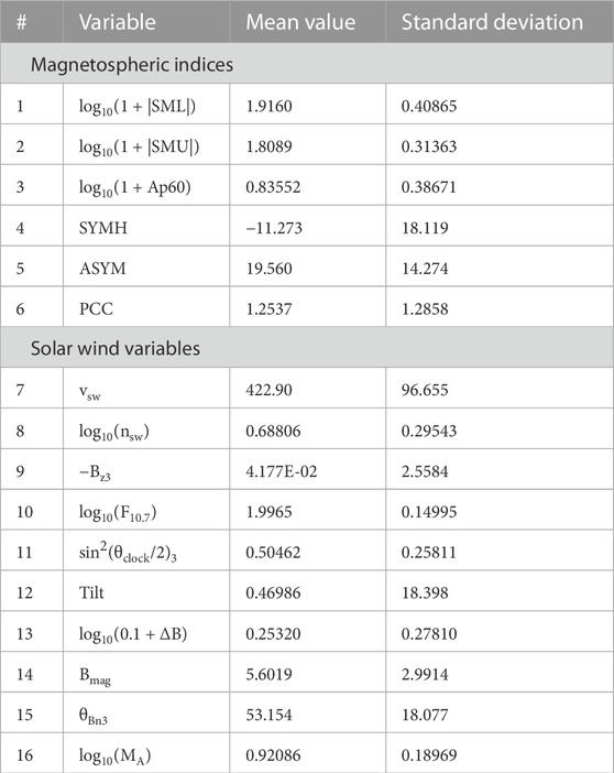
TABLE 3. Standardizing the variables for the 1997–2020 dataset [XX units].

The data used are available as follows: Ap60 is available at ftp://ftp.gfz-potsdam.de/pub/home/obs/Hpo. SML and SMU are available at http://supermag.jhuapl.edu/indices. SYMH, ASYM, and all solar wind variables are available at https://omniweb.gsfc.nasa.gov/. The PCC index is PCC = (PCN + PCS)/2 if PCN and PCS are both positive, PCC = PCN/2 if PCS is negative, PCC = PCS/2 if PCN is negative, and PCC = 0 if both PCN and PCS are negative (Stauning, 2021). PCN and PCS are available at http://isgi.unistra.fr.

The composite Earth index E₍₁₎(t) and its solar wind driver function S₍₁₎(t) are derived using canonical correlation analysis, which finds two projections (linear combinations) of the variables of each of the two datasets such that the two linear combinations E₍₁₎(t) and S₍₁₎(t) have the maximum Pearson linear correlation coefficient between each other. The two time-dependent multivariable datasets can be thought of as two time-dependent state vectors, and CCA can be thought of as the vector–vector correlation. CCA is a matrix (linear algebra) solution; it is not an iterative solver or a machine learning method. Data are not used to “train,” they are used to derive a solution. CCA is a well-known mathematical methodology (Muller, 1982; Johnson and Wichern, 2007; Gatignon, 2010; Nimon et al., 2010; Borovsky, 2014); it has often been used to identify causal factors or correlative factors, often in epidemiology ( Lassig and Duckett, 1979; Frie and Janssen, 2009). Recently, it has been adapted as a systems science tool for the reaction of complicated (multivariable) systems with time-dependent drivers, e.g., the time-dependent solar wind-driven magnetosphere–ionosphere system (Borovsky and Osmane, 2019).

4 The composite whole-Earth index E₍₁₎

Using the two sets of variables from Table 3 for the years 1997–2020, the CCA yields the two “first canonical variables” as the “Earth” index,

$\begin{array}{ll}\hfill {\mathrm{E}}_{\left(1\right)}& =0.1472{\log }_{10}\left(1+\left|\mathrm{S}\mathrm{M}\mathrm{L}\right|\right)*+0.2983{\log }_{10}\left(1+\left|\mathrm{S}\mathrm{M}\mathrm{U}\right|\right)*\hfill \\ \hfill & +0.3157{\log }_{10}\left(1+\mathrm{A}\mathrm{p}60\right)*-0.1108\mathrm{S}\mathrm{Y}\mathrm{M}\mathrm{H}*+0.1109\mathrm{A}\mathrm{S}\mathrm{Y}\mathrm{M}*\hfill \\ \hfill & +0.1987\mathrm{P}\mathrm{C}\mathrm{C}*\hfill \end{array},(1)$

and the “solar wind driver” of the Earth index as

$\begin{array}{c}{\mathrm{S}}_{\left(1\right)}=0.5707{{\mathrm{v}}_{\mathrm{s}\mathrm{w}}}^{*}+0.2284{\log }_{10}{\left({\mathrm{n}}_{\mathrm{s}\mathrm{w}}\right)}^{*}-0.4329{{\mathrm{B}}_{\mathrm{z}3}}^{*}+0.0909{\log }_{10}{\left({\mathrm{F}}_{10.7}\right)}^{*}\\ +0.2177{\sin }^2{\left({\mathrm{\theta }}_{\mathrm{c}\mathrm{l}\mathrm{o}\mathrm{c}\mathrm{k}}/2\right)}_{3^{*}}+0.1261{\mathrm{t}\mathrm{i}\mathrm{l}\mathrm{t}}^{*}+0.0956{\log }_{10}{\left(0.1+\Delta \mathrm{B}\right)}^{*}\\ +0.2590{\mathrm{B}}_{{\mathrm{m}\mathrm{a}\mathrm{g}}^{*}}+0.0757{\mathrm{\theta }}_{{\mathrm{B}\mathrm{n}3}^{*}}-0.0964{\log }_{10}{\left({\mathrm{M}}_{\mathrm{A}}\right)}^{*}\end{array}(2)$

Both E₍₁₎(t) and S₍₁₎(t) are time-dependent scalars. In Formulas 1, 2, the variables with asterisks are standardized: to standardize the variable X, the mean value of X is subtracted from X, and then the result is divided by the standard deviation of X so that the standardized variable X* has a mean value of 0, a standard deviation of unity, and no units. Hence, in expressions (1) and (2), the magnitudes of the coefficients of each standardized variable are indications of the “importance” or “contribution” of the variable to either E₍₁₎ or S₍₁₎. These coefficients (known as “weights”) are listed in the first two data columns of Table 4, and they are plotted in Figures 2A and B. As can be seen in Figure 2A, the contribution of SYMH and ASYM to E₍₁₎ is substantially weaker than that of the other four geomagnetic indices. Note in expression (1) the positive coefficient for the dipole tilt (tilt*), indicating that the solar wind statistically drives E₍₁₎ stronger when the northern hemisphere is tilted toward the Sun: this may be a result of the SML and SMU indices focusing on ground magnetometers in the northern hemisphere.

TABLE 4

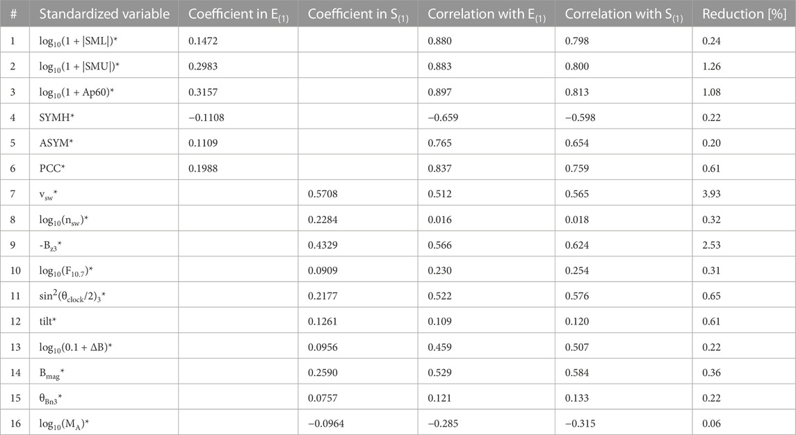
TABLE 4. Coefficients (weights) and correlations (loadings) for the variables going into E₍₁₎(t) and S₍₁₎(t) and the reduction (in percent) of the E₍₁₎(t) ↔ S₍₁₎(t) correlation when that variable is removed.

The factor’s mean value and standard deviation values used to standardize the hourly values of the 16 variables for the years 1997–2020 are listed in Table 3. Using these factors’ expressions, (1) and (2) are rewritten in terms of the 16 non-standardized variables as

$\begin{array}{ll}\hfill {\mathrm{E}}_{\left(1\right)}& =0.36022{\log }_{10}\left(1+\left|\mathrm{S}\mathrm{M}\mathrm{L}\right|\right)+0.95106{\log }_{10}\left(1+\left|\mathrm{S}\mathrm{M}\mathrm{U}\right|\right)\hfill \\ \hfill & +0.81583{\log }_{10}\left(1+\mathrm{A}\mathrm{p}60\right)-0.0061187\mathrm{S}\mathrm{Y}\mathrm{M}\mathrm{H}\hfill \\ \hfill & +0.0077747\mathrm{A}\mathrm{S}\mathrm{Y}\mathrm{M}+0.15468\mathrm{P}\mathrm{C}\mathrm{C}-3.5072\hfill \end{array}(3)$

and

$\begin{array}{ll}\hfill {\mathrm{S}}_{\left(1\right)}& =0.0059043{\mathrm{v}}_{\mathrm{s}\mathrm{w}}+0.77249{\log }_{10}\left({\mathrm{n}}_{\mathrm{s}\mathrm{w}}\right)-0.16923{\mathrm{B}}_{\mathrm{z}3}\hfill \\ \hfill & +0.60634{\log }_{10}\left({\mathrm{F}}_{10.7}\right)+0.84342{\sin }^2{\left({\mathrm{\theta }}_{\mathrm{c}\mathrm{l}\mathrm{o}\mathrm{c}\mathrm{k}}/2\right)}_3\hfill \\ \hfill & +0.0068518\mathrm{t}\mathrm{i}\mathrm{l}\mathrm{t}+0.34336{\log }_{10}\left(0.1+\Delta \mathrm{B}\right)+0.086675{\mathrm{B}}_{\mathrm{m}\mathrm{a}\mathrm{g}}\hfill \\ \hfill & +0.0041892{\mathrm{\theta }}_{\mathrm{B}\mathrm{n}3}-0.50686{\log }_{10}\left({\mathrm{M}}_{\mathrm{A}}\right)-5.0033\hfill \end{array}.(4)$

For expressions (3) and (4), the units of all variables are noted in Section 3.

The new composite magnetospheric activity index E₍₁₎(t) of expression (1) or (3) is plotted in Figure 3A as a function of its composite solar wind driver function S₍₁₎(t) given by expression (2) or (4) is plotted in Figure 3A, each black point being 1 h of data from the years 1997–2020. As a result of the CCA process that derived them, the values of E₍₁₎(t) and S₍₁₎(t) are standardized, with mean values of 0.00, standard deviations of 1.00, and no units. The standardization of E₍₁₎(t) means that E₍₁₎(t) <0 represents below-average magnetospheric activity and E₍₁₎(t) >0 represents above-average magnetospheric activity. Similarly, S₍₁₎(t) <0 represents below-average solar wind driving and S₍₁₎(t) >0 represents above-average driving. In Figure 3A, the Pearson linear correlation coefficient is r_corr = 0.907, meaning that only 1-r_corr² = 17.8% of the variance of E₍₁₎(t) is not described by a knowledge of S₍₁₎(t). It should be noted that this high correlation comes about without introducing time lags between solar wind variables and magnetospheric variables. An earlier study (Borovsky, 2020a) found that introducing and optimizing time lags between the magnetospheric variables and the solar wind variables do not significantly improve the results of the CCA process (the reason why time lags are not important in the CCA systems science methodology is not yet understood).

FIGURE 3

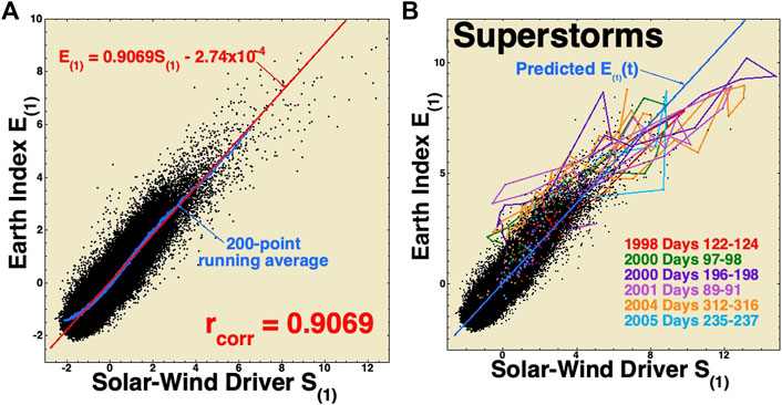
FIGURE 3. In panel (A), the data points for E₍₁₎ (t) are plotted as a function of S₍₁₎ (t) for the years 1997–2020. Each black point is 1 h of data. The red line is a linear regression fit to the black points, and the blue points are 200-point vertical running averages of the black points. In panel (B), the black points are replotted and the times of six superstorms are highlighted in six colors.

In Figure 3A, a least-squares linear regression fit is plotted as the blue line and a 200-point vertical running average is plotted as the red points. Note the linearity of the plot in Figure 3A, with the 200-point running average (blue) tracking the linear-regression fit (red). Using the linear-regression fit

${\mathrm{E}}_{\left(1\right)}\left(\mathrm{t}\right)=0.9069\mathrm{S}\left(1\right)\left(\mathrm{t}\right)-2.81\times {10}^{-4}(5)$

to predict E₍₁₎(t) from a knowledge of the value of S₍₁₎(t), the error E₍₁₎(t)–E_(1)predicted(t) is binned in Figure 4. The standard deviation of this distribution of errors is 0.446, and an error value of magnitude unity [which is one standard deviation of M(t)] is far on the tail of the distribution in Figure 4, with only 1.5% of the values having that magnitude of unity or greater. The prediction efficiency 1 - VAR(E_(1)predict(t)–E₍₁₎(t))/VAR(E₍₁₎(t)) = 82.2%. In Figure 4, it is noted that the standard deviations of E₍₁₎ and S₍₁₎ are both σ = 1.0, and the standard deviation of the error E₍₁₎(t)–E_(1)predicted is σ = 0.421.

FIGURE 4

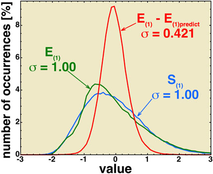
FIGURE 4. Values of E(t) (green), S₍₁₎(t) (blue), and the error E₍₁₎(t)–E_(1)predict(t) (red) are binned for the years 1997–2020 to form occurrence distributions.

It should be noted that using the CCA process composite magnetospheric indices E₍₁₎ can be derived that has higher correlations with their S₍₁₎ drivers if a larger diversity of measurements of the magnetosphere are included in the process, e.g., including ULF indices (Borovsky and Denton, 2014) or including particle population and particle precipitation measurements (Borovsky and Denton, 2018; Borovsky and Osmane, 2019). However, for the purpose of creating this community-useful composite index, the index must be based on measurement quantities that will be easily available in the future; hence, spacecraft-based measurements of particles and precipitation cannot be included.

It is known that some of the vertical error in the CCA-generated E₍₁₎ ↔ S₍₁₎ relationship is associated with the occurrence of substorms (Borovsky and Osmane, 2019), the timing of which is not predicted in the CCA process. This is shown in Figure 5, where 1,117 isolated substorms in the years 1997–2007 are used to create a superposed epoch average plot of E₍₁₎ and E₍₁₎–E_(1)predicted, with the zero epoch being the onset time of each substorm (substorm-onset collection is from Borovsky and Yakymenko (2017b), where the onsets were determined by a numerical algorithm that examines temporal changes in the 1-min-resolution SML index.). The lower curve in Figure 5 is E₍₁₎–E_(1)predicted, where E_(1)predicted is given by the linear regression fit of expression (5). Note in Figure 5 the increase in the magnitude of the error |E₍₁₎-E_(1)predicted| at the time of a substorm occurrence.

FIGURE 5

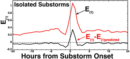
FIGURE 5. Superposed-epoch average plot of E₍₁₎ (black) and E₍₁₎–E_(1)predicted (red) with the zero epoch taken as the onset time of 1,117 isolated substorms.

Examining Figure 3A, it is noted that a slightly more accurate predictor equation for E₍₁₎ could possibly be created by using a curve fit to the 200-point running average in Figure 3A. Note the nonlinear curvature of the running average (blue) away from the linear-regression fit (red) in the bottom left portion of Figure 3A; it has been argued (Borovsky, 2021a) that this curvature might be owed to an atmospheric flywheel effect ( Richmond and Matsushita, 1975), wherein residual geomagnetic activity persists after solar wind driving ceases, owing to upper atmospheric convection driven by the prior activity; adding a time-integrated solar wind variable representing the past 10 h of driving by solar wind reduces the curvature.

5 Relative importance of individual geomagnetic indices and solar wind variables

The relative importance of the various individual variables in the CCA derivations of E₍₁₎ and S₍₁₎ can be judged by the magnitude of the variable’s coefficient in the expressions (1) and (2). These coefficients are listed in Table 4, and they are plotted in Figure 2. The CCA research literature ( Conger, 1974; Tzelgov and Henik, 1991; MacKinnon et al., 2000; Nimon et al., 2010; Hair et al., 2010) discusses further indications of the importance of the individual variables that can be gleaned by examining the correlations of the individual variables with E₍₁₎ and S₍₁₎ (known in the literature as “loadings”), in addition to examining the coefficients (known in the literature as “weights”). The correlations of the individual variables with the composites E₍₁₎ and S₍₁₎ are also listed in Table 4.

Another way to determine the relative importance of the individual variables is explored in the last column of Table 4, where the reduction in the percentage of the Pearson linear correlation coefficient between CCA-derived E₍₁₎ and S₍₁₎ composite variables is listed for cases where one geomagnetic index or one solar wind variable is eliminated from the CCA derivation procedure. This column provides further information about the importance of each index or each variable to the definition of E₍₁₎ and its solar wind driver S₍₁₎. In response to the solar wind, all geomagnetic variables act similarly to 0th order. Hence, as seen in the first six entries in the last column of Table 4, eliminating any one geomagnetic index from the CCA derivation of E₍₁₎ does not significantly reduce the correlation between E₍₁₎ and S₍₁₎.

Solar wind driver variables are different. The last column of Table 4 shows that if the value of v_sw is not known or if the value of B_z3 is not known, then the Pearson linear correlation coefficient between the CCA-derived composite variables E₍₁₎(t) and S₍₁₎(t) decreases very noticeably. According to Table 4, for the set of variables chosen, variables that have a more minor impact are ASYM in the Earth dataset and F_10.7, log₁₀(0.1+ΔB), B_mag, θ_Bn3, and log₁₀(M_A) in the solar wind dataset. It should be noted, however, that information carried in M_A is also carried in n_sw and B_mag. The contribution of the upstream magnetic field fluctuation amplitude ΔB to solar wind/magnetosphere coupling is controversial and is of interest in physics (Borovsky and Funsten, 2003; Osmane et al., 2015; D’Amicis et al., 2007; 2009; 2010; Borovsky, 2022c).

Among the individual geomagnetic variables and solar wind variables, there is also redundant information. This can be discerned in the CCA derivation process, where elimination of one variable results in a substantial increase in the CCA coefficient of the related variable. Exploration of this shows that for the Earth driving (1), B_mag and n_sw carry similar information (cf. Borovsky, 2018) and that for (2), B_mag, n_sw, and M_A are related (of course by the definition M_A = B_mag/(4πm_pn_sw)^1/2). Surprisingly, PCC and SML, which are both high-latitude indices that are highly correlated with each other, do not indicate that they are carrying similar information in the solar wind driving problem: eliminating one of these two variables does not result in a noticeable increase in the magnitude of the CCA coefficient of the other variable.

6 E₍₁₎ and the solar cycle and type of solar wind

In this section, the relations of E₍₁₎(t) to S₍₁₎(t), as defined by expressions (1) and (2), are examined in the different phases of the solar cycle and in the different types of solar wind plasma that drive the Earth’s magnetosphere.

The top panel of Figure 6 plots the yearly average values of E₍₁₎ (green) and the yearly average of S₍₁₎(t) (red). It should be noted that the value of E₍₁₎(t) is typically slightly less than the value of S₍₁₎ [see also expression (5)]. The bottom panel of Figure 6 plots the Pearson linear correlation coefficient r_corr between E₍₁₎(t) and S₍₁₎(t) for each year. It should be noted the drop in the value of r_corr around the year 2010 corresponds to weak activity E₍₁₎ and weak driving S₍₁₎ in the top panel. The years of weaker correlation in the bottom panel are probably owed to a common property of linear regression, wherein if the range of values of the points [e.g., S₍₁₎(t) and E₍₁₎(t)] becomes reduced (because of weak activity), the correlation coefficient tends to drop in magnitude ( Borovsky, 2022a), related to the property of “regression dilution bias” ( Liu, 1988; Hutcheon et al., 2010; Sivadas and Sibeck, 2022).

FIGURE 6

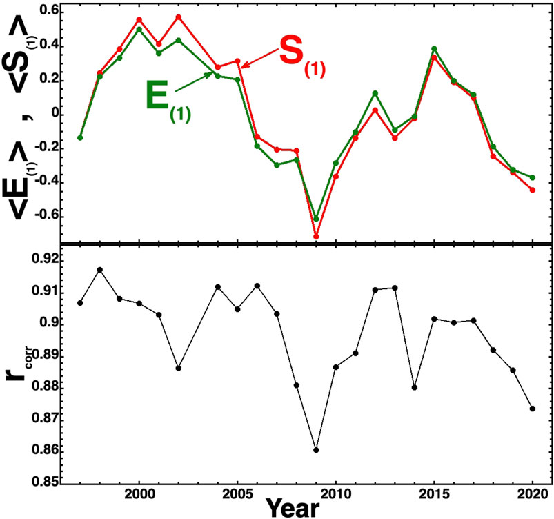
FIGURE 6. In the top panel, the yearly averages of E₍₁₎(t) (green) and S₍₁₎(t) (red) are plotted for years 1997–2020. In the bottom panel, the yearly Pearson linear correlation coefficient r_corr between E₍₁₎(t) and S₍₁₎(t) for each year is plotted.

In Figure 7A, 1997–2020 data are binned into four solar cycle phases and E₍₁₎(t) is plotted as a function of S₍₁₎(t) separately for each of the four phases, and a 100-point vertical running average of the data points is created. In Figure 7A, only the points of the four running averages are plotted, and the four running averages are color-coded as indicated in the figure. As can be seen in Figure 7A, the E₍₁₎ ↔ S₍₁₎ relationship is consistent between the various solar cycle phases.

FIGURE 7

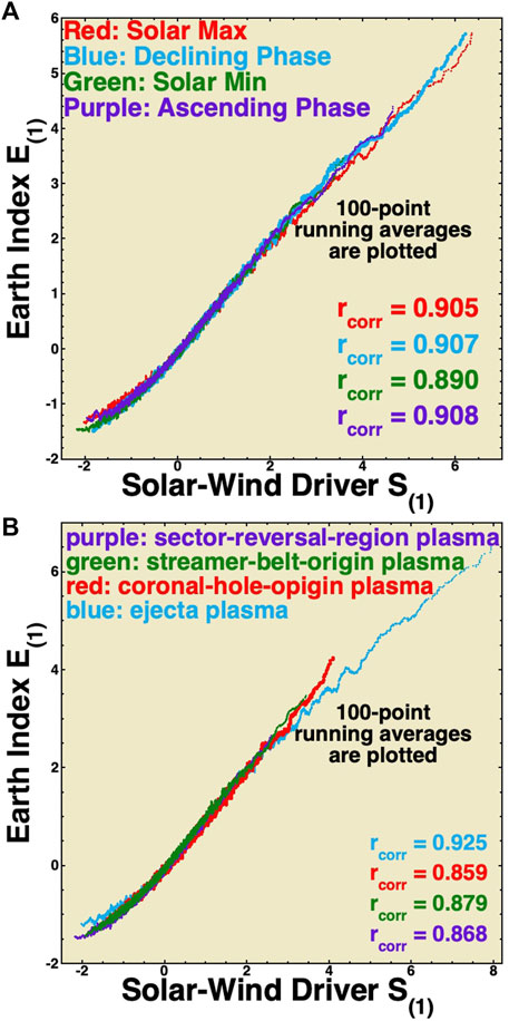
FIGURE 7. In panel (A), the 1997–2020 data are separated into the four phases of the solar cycle, and E₍₁₎ is plotted as a function of S₍₁₎ for the data in each phase (not shown) and 100-point running averages of the data in each phase are plotted in the four colors. In panel (B), the 1997–2020 data are separated into the types of solar wind plasma on Earth, and E₍₁₎ is plotted as a function of S₍₁₎ for the data in each type (not shown) and 100-point running averages of the data in each type are plotted in the four colors.

It should be noted that prior solar wind/magnetosphere coupling studies ( Nakai and Kamide, 1999; Nagatsuma, 2006; McPherron et al., 2009, McPherron et al., 2013) have argued that solar wind coupling changes the strength in the different phases of the solar cycle, i.e., that the ratio of geomagnetic activity to the solar wind driver function varies systematically with the phase of the solar cycle. The CCA-derived E₍₁₎ ↔ S₍₁₎ relationship does not show a solar cycle variation. With a better solar wind driver function S₍₁₎ and a better magnetospheric index E₍₁₎, no such solar cycle trend is seen. It should be noted that in Figure 7A, the Earth activity E₍₁₎ and solar wind driving S₍₁₎ do not go as high in magnitude during the solar minimum (green) as during other phases. In Figure 8A, the values of E₍₁₎ are again binned for each of the four solar cycles and the occurrence distributions are plotted, showing the weaker distribution of activity in the solar minimum (green).

FIGURE 8

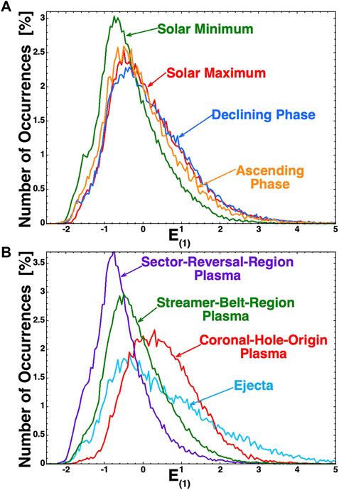
FIGURE 8. In panel (A), the 1997–2020 data are separated into the four phases of the solar cycle, and the values of E₍₁₎ are binned for the data in each phase to create occurrence distribution functions plotted in the four colors. In panel (B), the 1997–2020 data are separated into the types of solar wind plasma on Earth, and the values of E₍₁₎ are binned for the data in each type to create occurrence distribution functions plotted in the four colors.

In Figure 7B, the Xu and Borovsky (2015) solar wind categorization scheme is applied to each hour of the OMNI2 solar wind data in the years 1997–2020 to categorize each hour into the four types of solar wind plasma that bathe the Earth. As seen in Figure 7A, E₍₁₎ is plotted as a function of S₍₁₎ separately for the four types, and separate 100-point running averages are created and plotted for each of the four types. As labeled in Figure 7B, the four types of solar wind plasma are ejecta (blue), coronal hole-origin plasma (red), streamer belt-origin plasma (green), and sector reversal-region plasma (purple). The four types of solar wind plasma have systematically different properties concerning the driving of the Earth’s magnetosphere. Coronal hole-origin plasma is typically fast (high v_sw), with a low number density, weak magnetic field strength, high Alfvenicity, and its magnetic field orientation is Parker spiral-oriented. Streamer belt-origin plasma typically demonstrates medium speed and Alfvenicity, with the magnetic field Parker spiral-oriented. Sector reversal-region plasma is usually very slow, has high number density, and is non-Alfvenic, with a non-Parker spiral orientation of the magnetic field. Ejecta varies, but it can be extremely fast, with strong or weak magnetic field strength, low Alfven Mach numbers, and non-Parker spiral magnetic field orientations. The plotted running averages in Figure 7B indicate that the relationship between E₍₁₎(t) and S₍₁₎(t) is very similar for the four types of solar wind. It should be noted that in Figure 7B, ejecta plasma (blue) is capable of driving the magnetosphere to higher levels of activity [larger values of E₍₁₎]. This is also seen in Figure 8B, where the values of E₍₁₎ for the years 1997–2020 are binned into the four types of solar wind plasma and the occurrence distributions of E₍₁₎ values are plotted. The high E₍₁₎ tail on the ejecta distribution (light blue) is clearly seen. Note also the strong driving of E₍₁₎ in coronal-hole-origin plasma (red) and the weak driving of E₍₁₎ in sector-reversal-region plasma.

7 Using the new composite index E₍₁₎

In the left column of Figure 9, the superposed epoch averages of four quantities are plotted for 25 high-speed stream-driven storms from the collection of Borovsky and Denton (2016). The zero epoch (trigger) for the superposition is the MBI index (Gussenhoven et al., 1983; Madden and Gussenhoven, 1990), crossing 60.7^o equatorward (Borovsky and Denton, 2010), which is approximately when the magnetospheric convection index Kp exceeds 4.3 (cf. Borovsky and Denton, 2008). In the left column of Figure 9, the vertical red dashed line is the zero epoch where the high-speed stream-driven storms commence according to the MBI index. In the top two panels of Figure 9, the superposed average of the new composite magnetospheric index E₍₁₎ and its solar wind driver S₍₁₎ is plotted. As can be seen in E₍₁₎ index transitions from lower activity [E₍₁₎ ∼ 0] to high activity [E₍₁₎ >1] at the onset of storms. The behavior of the driver functions S₍₁₎ in the second panel reflects this. In the bottom two panels of Figure 9, the superposed averages of the two geomagnetic indices Hp60 (magnetospheric convection strength, similar to Kp) and SME (auroral activity) show their transitions from low activity to high activity. One takeaway from the left panel of Figure 9 is that a high-speed stream-driven geomagnetic storm might be defined as commencing when the magnetospheric index E₍₁₎ exceeds 1, which is one standard deviation of the E₍₁₎ distribution of values. For the years 1997–2020, E₍₁₎ is greater than the unity 15.4% of the time, which includes high-speed stream-driven storms, CME and CME-sheath driven storms, and other intervals of strong magnetospheric activity.

FIGURE 9

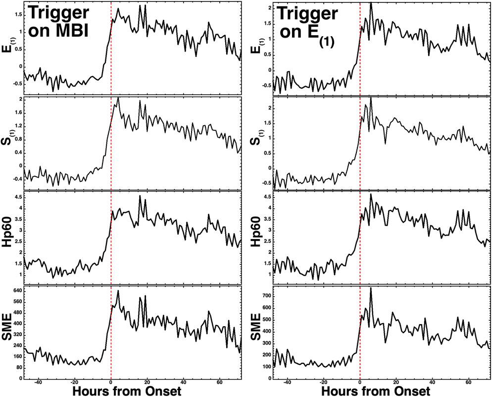
FIGURE 9. Superposed-epoch average plots for 25 high-speed stream-driven storms. In the left-hand column, the zero epoch for the superposition is the storm onset time as determined by the MBI index, and in the right-hand column, the zero epoch is the storm onset time determined as the time when E₍₁₎ first exceeds 1. The zero epoch is marked as the vertical red dashed line.

In the right column of Figure 9, the superposed-epoch averages of the quantities that were plotted in the left column are replotted with the zero epoch for the superposition chosen to be the time at which E₍₁₎ exceeds unity, a suggested new definition of storm activity. The plots of the right-hand Figure 9 are quite similar to the plots of the left column, where the zero epoch was triggered by the convective MBI index.

In Figure 10, the superposed-epoch average of the composite index E₍₁₎ is plotted for 43 CME-sheath-driven storms. The zero epoch is the time of shock passage at ACE at L1 upstream of the Earth. For these shocks, the magnetic cloud appears at ACE from 2.5–22 h after the shock; hence, the early part of the curve after the zero epoch is the uncontaminated sheath-driven storm data, and the later data are a mix of sheath-driven and cloud-driven storms. Comparing Figures 9, 10, it is seen that E₍₁₎ can be significantly higher for the sheath-driven storms than for the high-speed stream-driven storms. For high-speed stream-driven storms, E₍₁₎ is approximately 1 or more standard deviations from 0, whereas for sheath-driven storms, E₍₁₎ is 2 or more standard deviations from 0.

FIGURE 10

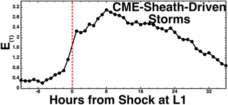
FIGURE 10. Superposed-epoch average plot of E₍₁₎ for 43 CME sheath-driven storms, where the zero epoch is the passage of the interplanetary shock ahead of each sheath as seen by the ACE spacecraft at L1.

In Figure 3B, the data of Figure 3A are replotted with the data from six superstorms (|SYMH| >250 nT) highlighted in six different colors. The hours just before and just after the superstorms are also plotted, with lines connecting the data points. The dark-blue line is the linear regression fit to E₍₁₎ as a function of S₍₁₎ (expression (5) for the entire 1997–2020 dataset). As can be seen, the data points of the superstorms track the linear regression fit quite well, with the linear regression blue line serving as a predictor of E₍₁₎ for a known value of S₍₁₎. The good tracking of the superstorm data to the prediction line may indicate that E₍₁₎(t) can be fairly well-predicted, even when as-yet-unseen extreme solar wind driving occurs, such as Carrington event driving (e.g., Li et al., 2006; Ngwira et al., 2014).

8 Future work

8.1 Exploring the S₍₁₎ driving of individual indices

As noted in Section 2, the CCA-derived solar wind driving function, S₍₁₎, can act as a universal driver function for geomagnetic activity with high correlations with individual geomagnetic indices and with magnetospheric particle populations [cf. Table 2 of Borovsky and Denton (2018)]. The quality of the S₍₁₎ universal driver derived here can be seen by examining the correlation coefficients listed in the first six entries of the second-to-last column of Table 4 (Note that these correlations are high, even without time lagging the indices from the solar wind). In future, the driving of other geomagnetic indices by this new S₍₁₎ should be explored. Furthermore, driving issues beyond the single global correlation coefficient should be examined [see also the warning by Lockwood (2022)], e.g., the correlation coefficients of data sorted by the solar cycle phase and the data sorted by the four types of solar wind plasma. Furthermore, questions about which geomagnetic indices saturate under strong driving (which is under low solar wind Mach numbers) in the driving of single indices by S₍₁₎ [cf. Figure 5 of Borovsky (2021a), which uses a different functional form for S₍₁₎ than the one given in this paper]. Using a different functional form for S₍₁₎, Borovsky (2021a) showed that in general, the individual indices exhibit less saturation when driven by a CCA-derived S₍₁₎ function than they do when driven by standard solar wind driver functions. An example of this is shown in Figure 11, using the new S₍₁₎ function of expression (2) or (4). In the top panel, the 1-h lagged SME index is plotted as a function of the solar wind driver R_quick (Borovsky and Birn, 2014), and in the bottom panel, the 1-hr-lagged SME index is plotted as a function of S₍₁₎. The plotted green points are 21-point running vertical averages of the full data. Linear regression fits are made to the full data from the 50th to the 90th percentile of the strength of the driver function; these fits are the red lines, with the red lines extending toward the top of the plots. As can be seen in Figure 11A, at large values of R_quick, the green running average curves downward away from the red line and flatten out; this is what is meant by “saturation” of the index under strong driving (Note also the saturation in both panels of Figure 1.) In Figure 11B, this flattening-out effect is seen to a lesser degree when SME is driven by the S₍₁₎ value introduced in Section 4, given by the expression (2) or (4). Note in Figure 11B the flattening of the SME curve for weak S(1) driving (similar to the flattening in Figure 3A): as discussed in Section 4, this might be owed to an atmospheric flywheel effect, where residual geomagnetic activity persists after solar wind driving ceases, owing to the inertia of atmospheric convection driven by the prior activity.

FIGURE 11

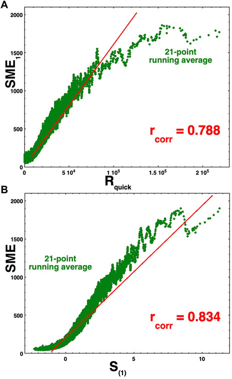
FIGURE 11. In panel (A), the 1-hr-lagged SME index is plotted (not shown) as a function of R_quick or the years 1997–2020, and a 21-point running average is created and plotted in green. In panel (B), the 1-hr-lagged SME index is plotted (not shown) as a function of S₍₁₎ or the years 1997–2020, and a 21-point running average is created and plotted in green. In both panels, linear regression fits are made (red line) for the 50th to 90th percentile of the driver strength, and then the regression line is extended toward the top of each plot.

8.2 The role of upstream solar wind fluctuations

Several studies have shown that geomagnetic activity levels are positively correlated with the amplitude of magnetic field fluctuations ΔB in the upstream solar wind (Borovsky and Funsten, 2003; Borovsky and Steinberg, 2008; Osmane et al., 2015; D’Amicis et al., 2007; D’Amicis et al., 2009; D’Amicis et al., 2010; D’Amicis et al., 2020). The question is whether there is a physical mechanism that underlies these correlations since ΔB could be acting as a proxy for other solar wind variables (Borovsky, 2022c). The CCA process, with the information it uncovers via the magnitudes of its coefficients and the strength of the index-versus-S₍₁₎ correlations (e.g., Table 4), can provide rich insight about the role of ΔB in the coupling process. Future versions of CCA based on information flow ( Wing et al., 2016; Wing and Johnson, 2019) rather than the Pearson linear correlation are under development; these versions will be particularly helpful in finding out how much ΔB drives the magnetosphere.

8.3 Explore the use of the projection state/vectors to identify different types of magnetospheric activity

One of our future goals would be to use E₍₁₎ to identify high-speed stream-driven activity, CME-driven activity, CME-cloud-driven activity, non-cloud ejecta-driven activity, etc., and to develop the critical E₍₁₎ level for the onset of different types of storms. Every time, a six-element state vector of magnetospheric activity can be created (SME*, SMU*, Ap60*, SYMH*, ASYM*, and PCC*). A pathway for a future project would be as follows: 1) to collect examples of known magnetospheric activity, 2) to create an average factor for each type of activity, and 3) for all other times the state vector of activity can be the dot product with the average state vector of each type of activity to see how close a vector is to one of the average vectors. Developing closeness criteria will allow magnetospheric activity to be categorized into one of the different types of activities.

8.4 Exploring the effects of noise and errors in the individual variables going into E₍₁₎ and S₍₁₎

Noise and/or errors in the solar wind variables and geomagnetic indices change the interpretation of how solar wind/magnetosphere coupling works, as seen in data analysis; noise lowers correlations and alters best-fit formulas of solar wind versus the geomagnetic index data (Borovsky, 2022a; Borovsky 2022b). Understanding how the coupling physically works is also made difficult by the multiple intercorrelations between all of the solar wind variables (Borovsky, 2020b; Borovsky 2021b). When fitting formulas by maximizing correlation coefficients, there are math-versus-physics reasons for the optimal correlations (Borovsky, 2021b). Noise in the solar wind variables comes, of course, from inaccuracies in the spacecraft measurements. The error in the solar wind measurements is much larger because, typically, the solar wind that hits an L1 monitor is not the solar wind that hits the Earth (Burkholder et al., 2020; Walsh et al., 2020). There is a triple dawn–dusk aberration that leads to the measured solar wind, typically missing the Earth off on the dusk side (Borovsky, 2022c). This is particularly bad for the small-scale magnetic structure of the solar wind that produces the on–off driving of the magnetosphere with sudden spatial changes in the solar wind magnetic field orientation. Additionally, geomagnetic indices are not perfect indicators of magnetospheric activity. A future project would be to explore the effects of noise and errors (a) in the S₍₁₎ ↔ E₍₁₎ derivation process and (b) in the behavior of the S₍₁₎ ↔ E₍₁₎ interactions for the E₍₁₎ and S₍₁₎ derived in Section 4.

Data availability statement

The original contributions presented in the study are included in the article/Supplementary Material; further inquiries can be directed to the corresponding author.

Author contributions

JB and CL performed all of the research and all of the writing of the manuscript. All authors contributed to the article and approved the submitted version.

Funding

JB was supported at the Space Science Institute by the NSF GEM program via grant AGS-2027569 and by the NASA HERMES Interdisciplinary Science program via grant 80NSSC21K1406. CL was funded at the Mullard Laboratory by the STFC studentship 2573668.

Acknowledgments

The authors thank Gian Luca Delzanno, Mick Denton, Adnane Osmane, and Peter Stauning. The authors also acknowledge GFZ Potsdam for the Ap60 index, which is available at ftp://ftp.gfz-potsdam.de/pub/home/obs/Hpo, and the authors acknowledge the SuperMAG team, where SuperMAG auroral electrojet indices are available at http://supermag.jhuapl.edu/indices. CL wishes to thank the Los Alamos National Laboratory for a Vela Fellowship, while attending the Los Alamos Space Weather Summer School.

Conflict of interest

The authors declare that the research was conducted in the absence of any commercial or financial relationships that could be construed as a potential conflict of interest.

Publisher’s note

All claims expressed in this article are solely those of the authors and do not necessarily represent those of their affiliated organizations, or those of the publisher, the editors, and the reviewers. Any product that may be evaluated in this article, or claim that may be made by its manufacturer, is not guaranteed or endorsed by the publisher.

References

Axford, W. I., and Hines, C. O. (1961). A unifying theory of high-latitude geophysical phenomena and geomagnetic storms Canadian. J. Phys. 39, 1433–1464. doi:10.1139/p61-172

CrossRef Full Text | Google Scholar

Borovsky, J. E. (2020a). A survey of geomagnetic and plasma time lags in the solar-wind-driven magnetosphere of Earth. J. Atmos. Solar-Terr. Phys. 208, 105376. doi:10.1016/j.jastp.2020.105376

CrossRef Full Text | Google Scholar

Borovsky, J. E., and Birn, J. (2014). The solar-wind electric field does not control the dayside reconnection rate. J. Geophys. Res. 119, 751–760. doi:10.1002/2013ja019193

CrossRef Full Text | Google Scholar

Borovsky, J. E. (2014). Canonical correlation analysis of the combined solar-wind and geomagnetic-index data sets. J. Geophys. Res. 119, 5364–5381. doi:10.1002/2013ja019607

CrossRef Full Text | Google Scholar

Borovsky, J. E., and Denton, M. H. (2016). Compressional perturbations of the dayside magnetosphere during high-speed-stream-driven geomagnetic storms. J. Geophys. Res. 121, 4569–4589. doi:10.1002/2015ja022136

CrossRef Full Text | Google Scholar

Borovsky, J. E., and Denton, M. H. (2006). Differences between CME-driven storms and CIR-driven storms. J. Geophys. Res. 111, A07S08. doi:10.1029/2005ja011447

CrossRef Full Text | Google Scholar

Borovsky, J. E., and Denton, M. H. (2018). Exploration of a composite index to describe magnetospheric activity: reduction of the magnetospheric state vector to a single scalar. J. Geophys. Res. 123, 7384–7412. doi:10.1029/2018ja025430

CrossRef Full Text | Google Scholar

Borovsky, J. E., and Denton, M. H. (2014). Exploring the cross-correlations and autocorrelations of the ULF indices and incorporating the ULF indices into the systems science of the solar-wind-driven magnetosphere. J. Geophys. Res. 119, 4307–4334. doi:10.1002/2014ja019876

CrossRef Full Text | Google Scholar

Borovsky, J. E., and Denton, M. H. (2010). The magnetic field at geosynchronous orbit during high-speed-stream-driven storms: connections to the solar wind, the plasma sheet, and the outer electron radiation belt. J. Geophys. Res. 115, a08217. doi:10.1029/2009JA015116

CrossRef Full Text | Google Scholar

Borovsky, J. E., and Funsten, H. O. (2003). Role of solar wind turbulence in the coupling of the solar wind to the Earth's magnetosphere. J. Geophys. Res. 108, 1246. doi:10.1029/2002ja009601

CrossRef Full Text | Google Scholar

Borovsky, J. E., Lavraud, B., and Kuznetsova, M. M. (2009). Polar cap potential saturation, dayside reconnection, and changes to the magnetosphere. J. Geophys. Res. 114, a03224. doi:10.1029/2009ja014058

CrossRef Full Text | Google Scholar

Borovsky, J. E. (2022b). Noise and solar-wind/magnetosphere coupling: data. Front. Astron. Space Sci. 9, 990789. doi:10.3389/fspas.2022.990789

CrossRef Full Text | Google Scholar

Borovsky, J. E. (2022a). Noise, regression dilution bias, and solar-wind/magnetosphere coupling studies. Front. Astron. Space Sci. 9, 867282. doi:10.3389/fspas.2022.867282

CrossRef Full Text | Google Scholar

Borovsky, J. E. (2018). On the origins of the intercorrelations between solar wind variables. J. Geophys. Res. 123, 20–29. doi:10.1002/2017ja024650

CrossRef Full Text | Google Scholar

Borovsky, J. E. (2021a). On the saturation (or not) of geomagnetic indices. Front. Astron. Space Sci. 8, 740811. doi:10.3389/fspas.2021.740811

CrossRef Full Text | Google Scholar

Borovsky, J. E., and Osmane, A. (2019). Compacting the description of a time-dependent multivariable system and its multivariable driver by reducing the state vectors to aggregate scalars: the Earth's solar-wind-driven magnetosphere. Nonlin. Process. Geophys 26, 429–443. doi:10.5194/npg-26-429-2019

CrossRef Full Text | Google Scholar

Borovsky, J. E. (2021b). Perspective: is our understanding of solar-wind/magnetosphere coupling satisfactory? Front. Astron. Space Sci. 8, 634073. doi:10.3389/fspas.2021.634073

CrossRef Full Text | Google Scholar

Borovsky, J. E. (2013). Physics based solar-wind driver functions for the magnetosphere: combining the reconnection-coupled MHD generator with the viscous interaction. J. Geophys. Res. 118, 7119–7150. doi:10.1002/jgra.50557

CrossRef Full Text | Google Scholar

Borovsky, J. E., and Shprits, Y. (2017a). Is the Dst index sufficient to define a storm? J. Geophys. Res. 122, 11543. doi:10.1002/2017JA024679

CrossRef Full Text | Google Scholar

Borovsky, J. E., and Steinberg, J. T. (2006). “The freestream turbulence effect in solar-wind/magnetosphere coupling: analysis through the solar cycle and for various types of solar wind,” in Recurrent magnetic storms: Cororating solar wind streams (Washington, United States: American Geophysical Union), 59.

CrossRef Full Text | Google Scholar

Borovsky, J. E. (2008). The rudiments of a theory of solar-wind/magnetosphere coupling derived from first principles. J. Geophys. Res. 113, a08228. doi:10.1029/2007ja012646

CrossRef Full Text | Google Scholar

Borovsky, J. E. (2022c). The triple dusk-dawn aberration of the solar wind at Earth. Front. Astron. Space Sci. 9, 917163. doi:10.3389/fspas.2022.917163

CrossRef Full Text | Google Scholar

Borovsky, J. E., and Valdivia, J. A. (2018). The Earth’s magnetosphere: a systems science overview and assessment. Surv. Geophys 39, 817–859. doi:10.1007/s10712-018-9487-x

PubMed Abstract | CrossRef Full Text | Google Scholar

Borovsky, J. E. (2020b). What magnetospheric and ionospheric researchers should know about the solar wind. J. Atmos. Solar-Terr. Phys. 204, 105271. doi:10.1016/j.jastp.2020.105271

CrossRef Full Text | Google Scholar

Borovsky, J. E., and Yakymenko, K. (2017b). Systems science of the magnetosphere: creating indices of substorm activity, of the substorm-injected electron population, and of the electron radiation belt. J. Geophys. Res. 122, 10012–10,035. doi:10.1002/2017ja024250

CrossRef Full Text | Google Scholar

Burkholder, B. L., Nykyri, K., and Ma, X. (2020). Use of the L1 constellation as a multispacecraft solar wind monitor. J. Geophys. Res. 125, e2020JA027978. doi:10.1029/2020ja027978

CrossRef Full Text | Google Scholar

Conger, A. J. (1974). A revised definition for suppressor variables: a guide to their identification and interpretation. Educ. Psychol. Meas. 34, 35–46. doi:10.1177/001316447403400105

CrossRef Full Text | Google Scholar

D’Amicis, R., Bruno, R., and Bavassano, B. (2009). Alfvénic turbulence in high speed solar wind streams as a driver for auroral activity. J. Atmos. Sol. -Terr. Phys. 71, 1014–1022. doi:10.1016/j.jastp.2008.05.002

CrossRef Full Text | Google Scholar

D’Amicis, R., Bruno, R., and Bavassano, B. (2010). Geomagnetic activity driven by solar wind turbulence. Adv. Space Res. 46, 514–520. doi:10.1016/j.asr.2009.08.031

CrossRef Full Text | Google Scholar

D’Amicis, R., Bruno, R., and Bavassano, B. (2007). Is geomagnetic activity driven by solar wind turbulence? Geophys. Res. Lett. 34, l05108. doi:10.1029/2006gl028896

CrossRef Full Text | Google Scholar

D’Amicis, R., Telloni, D., and Bruno, R. (2020). The effect of solar-wind turbulence on magnetospheric activity. Front. Phys. 8, 604857. doi:10.3389/fphy.2020.604857

CrossRef Full Text | Google Scholar

Dungey, J. W. (1961). Interplanetary magnetic field and the auroral zones. Phys. Rev. Lett. 6, 47–48. doi:10.1103/physrevlett.6.47

CrossRef Full Text | Google Scholar

Frie, K. G., and Janssen, C. (2009). Social inequality, lifestyles and health – A non-linear canonical correlation analysis based on the approach of pierre bourdieu. Int. J. Public Health 54, 213–221. doi:10.1007/s00038-009-8017-5

PubMed Abstract | CrossRef Full Text | Google Scholar

Gatignon, H. (2010). Statistical analysis of management data. New York: Springer.

Google Scholar

Gjerloev, J. W. (2012). The SuperMAG data processing technique. J. Geophys. Res. 117, a09213. doi:10.1029/2012ja017683

CrossRef Full Text | Google Scholar

Gussenhoven, M. S., Hardy, D. A., and Heinemann, N. (1983). Systematics of the equatorward diffuse auroral boundary. J. Geophys. Res. 88, 5692. doi:10.1029/ja088ia07p05692

CrossRef Full Text | Google Scholar

Hair, J. F., Black, W. C., Babin, B. J., and Anderson, R. E. (2010). Canonical correlation: A supplement to multivariate data analysis. Upper Saddle River, NJ: Pearson Prentice Hall Publishing.

Google Scholar

Hoilijoki, S., Souza, V. M., Walsh, B. M., Janhunen, P., and Palmroth, M. (2014). Magnetopause reconnection and energy conversion as influenced by the dipole tilt and the IMF B_x. J. Geophys. Res. 119, 4484–4494. doi:10.1002/2013ja019693

CrossRef Full Text | Google Scholar

Holzer, R. E., and Slavin, J. A. (1982). An evaluation of three predictors of geomagnetic activity. J. Geophys. Res. 87, 2558. doi:10.1029/ja087ia04p02558

CrossRef Full Text | Google Scholar

Hutcheon, J. A., Chiolero, A., and Hanley, J. A. (2010). Random measurement error and regression dilution bias. BMJ 340, c2289–c1406. doi:10.1136/bmj.c2289

PubMed Abstract | CrossRef Full Text | Google Scholar

Johnson, R. A., and Wichern, D. W. (2007). Applied multivariate statistical analysis. 6. Upper Saddle River, New Jersey: Pearson Prentice Hall.

Google Scholar

King, J. H., and Papitashvili, N. E. (2005). Solar wind spatial scales in and comparisons of hourly Wind and ACE plasma and magnetic field data. J. Geophys. Res. 110, 2104. doi:10.1029/2004JA010649

CrossRef Full Text | Google Scholar

Lassig, R. E., and Duckett, E. J. (1979). Canonical correlation analysis: potential for environmental health planning. Am. J. Public Health 54, 213.

Google Scholar

Lavraud, B., and Borovsky, J. E. (2008). Altered solar wind-magnetosphere interaction at low Mach numbers: coronal mass ejections. J. Geophys. Res. 113, a00B08. doi:10.1029/2008ja013192

CrossRef Full Text | Google Scholar

Li, X., Temerin, M., Tsurutani, B. T., and Alex, S. (2006). Modeling of 1-2 September 1859 super magnetic storm. Adv. Space Res. 38, 273–279. doi:10.1016/j.asr.2005.06.070

CrossRef Full Text | Google Scholar

Liu, K. (1988). Measurement error and its impact on partial correlation and multiple linear regression analysis. Amer. Jour. Epidemiol. 127, 864–874. doi:10.1093/oxfordjournals.aje.a114870

PubMed Abstract | CrossRef Full Text | Google Scholar

Lockwood, M., and McWilliams, K. A. (2021). On optimum solar wind-magnetosphere coupling functions for transpolar voltage and planetary geomagnetic activity. J. Geophys. Res. 126, e2021JA029946. doi:10.1029/2021ja029946

CrossRef Full Text | Google Scholar

Lockwood, M. (2022). Solar wind--magnetosphere coupling functions: pitfalls, limitations, and applications. Space Weath 20, e2021SW002989. doi:10.1029/2021sw002989

CrossRef Full Text | Google Scholar

Loewe, C. A., and Prolss, G. W. (1997). Classification and mean behavior of magnetic storms. J. Geophys. Res. 102, 14209–14213. doi:10.1029/96ja04020

CrossRef Full Text | Google Scholar

Luo, A. C. J. (2010). Dynamical systems. New York: Springer.

Google Scholar

MacKinnon, D. P., Krull, J. L., and Lockwood, C. M. (2000). Equivalence of the mediation, confounding, and suppression effect. Prev. Sci. 1, 173–181. doi:10.1023/a:1026595011371

PubMed Abstract | CrossRef Full Text | Google Scholar

Madden, D., and Gussenhoven, M. S. (1990). Auroral boundary index from 1983 to 1990, tech report GL-TR-90-0358. Hanscom AFB, MA: Air Force Geophysics Laboratory.

Google Scholar

McPherron, R. L., Baker, D. N., Pulkkinen, T. I., Hsu, T.-S., Kissinger, J., and Chu, X. (2013). Changes in solar wind-magnetosphere coupling with solar cycle, season, and time relative to stream interfaces. J. Atmos. Solar-Terr. Phys. 99, 1–13. doi:10.1016/j.jastp.2012.09.003

CrossRef Full Text | Google Scholar

McPherron, R. L., Hsu, T.-S., and Chu, X. (2015). An optimum solar wind coupling function for the AL index. J. Geophys. Res. 120-2494, 2494–2515. doi:10.1002/2014ja020619

CrossRef Full Text | Google Scholar

McPherron, R. L., Kepko, L., Pulkkinen, T. I., Hsu, T. S., Weygand, J. W., and Bargatze, L. F. (2009). Changes in the response of the AL index with solar cycle and epoch within a corotating interaction region. Ann. Geophys. 27, 3165–3178. doi:10.5194/angeo-27-3165-2009

CrossRef Full Text | Google Scholar

Muller, K. E. (1982). Understanding canonical correlation through the general linear model and principal components. Amer. Stat. 36, 342. doi:10.2307/2683082

CrossRef Full Text | Google Scholar

Myllys, M., Kipua, E. K. J., and Lavraud, B. (2017). Interplay of solar wind parameters and physical mechanisms producing the saturation of the cross polar cap potential. Geophys. Res. Lett. 44, 3019–3027. doi:10.1002/2017gl072676

CrossRef Full Text | Google Scholar

Nagatsuma, T. (2006). Diurnal, semiannual, and solar cycle variations of solar wind-magnetosphere-ionosphere coupling. J. Geophys. Res. 111, A09202. doi:10.1029/2005ja011122

CrossRef Full Text | Google Scholar

Nakai, H., and Kamide, Y., (1999). Solar cycle variations in the storm-substorm relationship. J. Geophys. Res. 104, 22695–22700. doi:10.1029/1999ja900278

CrossRef Full Text | Google Scholar

Newell, P. T., Sotirelis, T., Liou, K., Meng, C. I., and Rich, F. J. (2007). A nearly universal solar wind-magnetosphere coupling function inferred from 10 magnetospheric state variables. J. Geophys. Res. 112, A01206. doi:10.1029/2006ja01-2015

CrossRef Full Text | Google Scholar

Newell, P. T., Sotirelis, T., Liou, K., and Rich, F. J. (2008). Pairs of solar wind-magnetosphere coupling functions: combining a merging term with a viscous term works best. J. Geophys. Res. 113, A04218. doi:10.1029/2007ja012825

CrossRef Full Text | Google Scholar

Ngwira, C. M., Pulkkinen, A., Kusnetsova, M. M., and Glocer, A. (2014). Modeling extreme “Carrington-type” space weather events using three-dimensional global MHD simulations. J. Geophys. Res. 119, 4456–4474. doi:10.1002/2013ja019661

CrossRef Full Text | Google Scholar

Nimon, K., Henson, R. K., and Gates, M. S. (2010). Revisiting interpretation of canonical correlation analysis: a tutorial and demonstration of canonical commonality analysis. Multivar. Behav. Res. 45, 702–724. doi:10.1080/00273171.2010.498293

PubMed Abstract | CrossRef Full Text | Google Scholar

Nowada, M., Shue, J.-H., and Russell, C. T. (2009). Effects of dipole tilt angle on geomagnetic activity. Space Sci. 57, 1254–1259. doi:10.1016/j.pss.2009.04.007

CrossRef Full Text | Google Scholar

Osmane, A., Dimmock, A. P., Naderpour, R., Pulkkinen, T. I., and Nykyri, K. (2015). The impact of solar wind ULF B_z fluctuations on geomagnetic activity for viscous timescales during strongly northward and southward IMF. J. Geophys. Res. 120, 9307–9322. doi:10.1002/2015ja021505

CrossRef Full Text | Google Scholar

Reiff, P. H., and Luhmann, J. G. (1986). “Solar wind control of the polar-cap voltage,” in Solar wind-magnetosphere coupling. Editors Y. Kamide, and J. A. Slavin (Tokyo: Terra Scientific), 453.

CrossRef Full Text | Google Scholar

Richmond, A. D., and Matsushita, S. (1975). Thermospheric response to a magnetic substorm. J. Geophys. Res. 80, 2839–2850. doi:10.1029/ja080i019p02839

CrossRef Full Text | Google Scholar

Sivadas, N., and Sibeck, D. G. (2022). Regression bias in using solar wind measurements. Front. Astron. Space Sci. 9, 924978. doi:10.3389/fspas.2022.924976

CrossRef Full Text | Google Scholar

Stauning, P. (2021). The polar cap (PC) index combination, PCC: relations to solar wind properties and global magnetic disturbances. J. Space Weather Space Clim. 11, 19. doi:10.1051/swsc/2020074

CrossRef Full Text | Google Scholar

Sugiura, M., and Chapman, S. (1960). The average morphology of geomagnetic storms with sudden commencement. Göttingen: Sondernheft Nr.4. Abandl. Akad. Wiss. Göttingen Math. Phys. Kl.

Google Scholar

Tzelgov, J., and Henik, A. (1991). Suppression situations in psychological research: definitions, implications, and applications. Bull 109, 524–536. doi:10.1037/0033-2909.109.3.524

CrossRef Full Text | Google Scholar

Vassiliadis, D. (2006). Systems theory for geospace plasma dynamics. Rev. Geophys. 44, RG2002. doi:10.1029/2004rg000161

CrossRef Full Text | Google Scholar

Walsh, B. M., Bhakyapaibul, T., and Zou, Y. (2020). Quantifying the uncertainty of using solar wind measurements for geospace inputs. J. Geophys. Res. 124, 3291–3302. doi:10.1029/2019ja026507

CrossRef Full Text | Google Scholar

Weimer, D. R., Reinleitner, L. A., Kan, J. R., Zhu, L., and Akasofu, S.-I. (1990). Saturation of the auroral electrojet current and the polar cap potential. J. Geophys. Res. 95, 18981. doi:10.1029/ja095ia11p18981

CrossRef Full Text | Google Scholar

Wing, S., and Johnson, J. R. (2019). Applications of information theory in solar and space physics. Entropy 21, 140. doi:10.3390/e21020140

PubMed Abstract | CrossRef Full Text | Google Scholar

Wing, S., Johnson, J. R., Camporeale, E., and Reeves, G. D. (2016). Information theoretical approach to discovering solar wind drivers of the outer radiation belt. J. Geophys. Res. 121, 9378–9399. doi:10.1002/2016ja022711

CrossRef Full Text | Google Scholar

Wygant, J. R., Torbert, R. B., and Mozer, F. S. (1983). Comparison of S3-3 polar cap potential drops with the interplanetary magnetic field and models of magnetopause reconnection. J. Geophys. Res. 88, 5727. doi:10.1029/ja088ia07p05727

CrossRef Full Text | Google Scholar

Xu, F., and Borovsky, J. E., (2015). A new four-plasma categorization scheme for the solar wind: 4-Plasma solar-wind categorization. J. Geophys. Res. 120, 70–100. doi:10.1002/2014ja020412

CrossRef Full Text | Google Scholar