 Russell A. Howard
 Angelos Vourlidas
 Guillermo Stenborg
- Applied Physics Laboratory, Johns Hopkins University, Laurel, MD, United States
The unexpected observation of a sudden expulsion of mass through the solar corona in 1971 opened up a new field of interest in solar and stellar physics. The discovery came from a white-light coronagraph, which creates an artificial eclipse of the Sun, enabling the viewing of the faint glow from the corona. This observation was followed by many more observations and new missions. In the five decades since that discovery, there have been five generations of coronagraphs, each with improved performance, enabling continued understanding of the phenomena, which became known as Coronal Mass Ejection (CME) events. The conceptualization of the CME structure evolved from the elementary 2-dimensional loop to basically two fundamental types: a 3-dimensional magnetic flux rope and a non-magnetic eruption from pseudo-streamers. The former persists to 1 AU and beyond, whereas the latter dissipates by 15 R⊙. Historically, most of the studies have been devoted to understanding the CME large-scale structure and its associations, but this is changing. With the advent of the fourth and fifth coronagraph generations, more attention is being devoted to the their internal structure and initiation mechanisms. In this review, we describe the evolution of CME observations and their associations with other solar and heliospheric phenomena, with one of the more important correlations being its recognition as a driver of space-weather. We conclude with a brief overview of open questions and present some ideas for future observations.
1 Introduction
We present an historical overview of the significant milestones in Coronal Mass Ejection (CME) research that led to our current understanding of the CME process. There have been over 20,000 papers on CMEs, so this is a consequential field of research. It is also personal, since one of us (RAH) joined the U.S. Naval Research Laboratory (NRL) coronagraph group a week after the launch of the spacecraft that observed the first direct evidence of mass leaving the Sun. That observation spawned a truly international research effort.
The white-light coronagraph (WLC) is the instrument which best observes the medium (i.e., the solar corona) the CME is traveling through. This type of instrument deals with the detection of a faint signal very close to a bright source. In a nutshell, they work by blocking out the light from the solar disk, creating an artificial eclipse of the Sun. A hindrance to this invention is that the occulter used to block out the Sun generates a lot of stray light. The stray light problem was first tackled by Lyot (1932) enabling ground based telescopes to observespectral lines in the corona just off the limb of the Sun. Later, Wlérick and Axtell (1957) added polarizers to the Lyot design to allow the detection of the electron corona (i.e., the so-called K-corona) further out by suppressing the contribution of the unpolarized F-corona (i.e., photospheric light scattered by the dust particles revolving around the Sun). But that still was not as far out into the corona as eclipses allow.
Evans (1948) developed the concept of adding an external occulter onto a Lyot coronagraph, which required an internal occulter and some additional Lyot type apertures to suppress the stray light. Newkirk and Eddy (1962) flew such an externally occulted Lyot coronagraph on a high-altitude balloon, obtaining very good coronal profiles from 40,000 to 80,000 feet. Unfortunately, the imaging did not work due to excessive scattered light from the single external occulter disk. Later on, Tousey (1965) reported the first successful imaging of the solar corona outside of an eclipse from an Aerobee rocket flight on 28 June 1963 (Koomen et al., 1964). The rocket carried an externally occulted Lyot coronagraph, in which the single occulter was a serrated design developed by Purcell and Koomen (1962), who showed that it was more effective in reducing the stray light than the single disk with a smooth edge. Newkirk and Bohlin (1963) investigated the stray light reduction using three concentric disks rather than one demonstrating the effectiveness of it in a later high-altitude balloon experiment (Newkirk and Bohlin, 1965). The later coronagraphs, e.g., those onboard the OSO-7 satelite (Koomen et al., 1975, see also Section 2.1) have almost exclusively used the triple disk with smooth edges, because they are much easier to clean as well as fabricate.
CMEs have been best observed in visible wavelengths by a WLC or its cousin, the heliospheric imager (HI). A coronagraph occults the Sun using a circular occulter, thereby showing the entire corona surrounding the disk, whereas the HI uses a linear occulter assembly to occult the solar disk, thereby showing only one hemisphere. As will be shown later, extreme-ultraviolet (EUV) imaging observations are well suited to observe the very critical initiation and low coronal manifestations of the CME events. On the other hand, the observations from the WLC or HI are better suited to show the evolution of the events’ morphology and kinematics as they leave the Sun and evolve in the low and middle corona.
Table 1 gives a timeline of all of the spacecraft missions that have been launched and carried either a WLC or HI instrument. We have chosen to describe the results along with the evolution of the instrument technology, which have virtually followed a decadal evolution. In each decade since 1970 there were one or two missions that carried coronagraph(s). In the following we will refer to them as Generation 1 (1970s), Generation 2 (1980s), Generation 3 (1990s), Generation 4 (2000s), and Generation 5 (2010s).
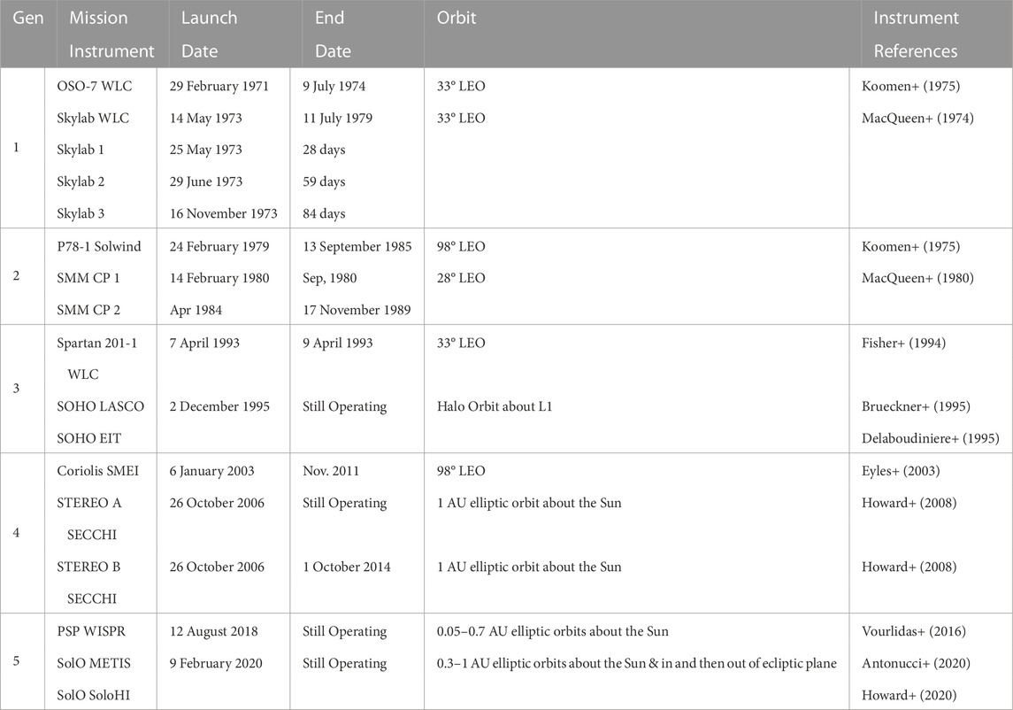
TABLE 1. Generations of white-light Coronagraphs and Heliospheric Imagers.
2 First generation missions - 1970s
2.1 OSO-7
On 29 December 1971, the National Aeronautics and Space Administration (NASA) launched the 7th in the series of Orbiting Solar Observatories (OSO-7). This series of spacecraft consisted of a rotating wheel section and a despun section pointed at the Sun. The wheel section contained the spacecraft electronics and instruments which did not need pointing such as the in-situ instruments that measure the local solar wind. The despun section contained the solar array(s) and two remote sensing instruments. One of the OSO-7 sun-pointed instruments was a combined WLC (Koomen et al., 1975) and Extreme Ultraviolet (EUV) coronagraph ((XUVC) Michels and Tousey, 1971). The other sun-pointed instrument was an EUV and X-Ray Spectroheliograph (Underwood and Neupert, 1974). The XUVC and EUV/X-Ray instruments would build up an image by rastering the pointed section across the solar disk. A WLC observes the photospheric light Thomson-scattered by the free electrons in the corona/solar wind. The scattering is optically thin, so that the detection is an integration of the scattering all along the line of sight for each pixel, (see, e.g., Vourlidas and Howard, 2006). This was the first instance of such an instrument being flown on a spacecraft. The impetus for this may have been due to a pair of identical rockets launched on successive days in the mid 1960s by Martin Koomen with his team. The images showed significant evolution in the coronal structure, which was thought to change on solar cycle scales up to that point. Naturally, these observations raised the question: How does this happen?
The OSO-7 WLC was an instrument similar to the rocket instruments (Koomen et al., 1970; Bohlin et al., 1971), i.e., an externally-occulted Lyot coronagraph with a field of view (FOV) of the solar corona from 3 to 10 R⊙. The light from the solar disk was blocked out by an external disk assembly of three concentric disks with smooth edges. For the spacecraft version of this instrument, the film was not an option as the detector, so they used instead a new (for space) Secondary Electron Conduction (SEC) Vidicon (Tousey and Limansky, 1972; Zucchino and Lowrance, 1972) to record the coronal intensity. The Vidicon detector was read out with 256 × 256 pixels and 7-bit/pixel intensity resolution. The spatial resolution was 1.25 arcmin/pixel. There were two modes of data compression—sending down only a quadrant of the image, and a run-length encoding scheme which sent down the full intensity and then the number of consecutive pixels that were within a preselected corridor of the initial pixel. There were several different corridors of different widths. The most significant bit of each byte was used to signify whether the data byte was an intensity or run-length.
A safety concern arose early in the operations of the two sun-pointed instruments. The WLC required sun-centered pointing, whereas the other would off-point from sun-center or scan across the Sun. This resulted in the WLC operating for 4 consecutive orbits out of the 15 per day. The bit rate of the WLC was 200 bits/sec, which allowed about 1 image to be read out per orbit. The run-length and quadrant allowed more images to be collected, but at the expense of scene coverage or reduced intensity resolution.
The OSO-7 mission duration was planned to be 1 year, but it actually lasted for over 4 years. Problems during the launch created a bad elliptic orbit and the spacecraft re-entered the atmosphere on 9 July 1974 (see Table 1); but effectively, the mission ended in 1973 due to failures in various subsystems, including the tape recorder.
Figure 1, panels (a) through (f), show the sequence of direct intensity images collected on December 13-14, 1971 of the first CME event captured by the instrument, and panels (g) through (l) show the same image sequence with a pre-event base image subtracted from them. This event was a total surprise as no one had ever expressed such a possibility. Erupting filaments or prominences had been known to slowly lift off the surface, but the general consensus was that the material drained back because they were not anywhere close to the speed needed to escape the solar gravity. On seeing the first few images, a concern was that the SEC Vidicon, which was very sensitive to excessive vibration and intensities, had suffered some damage, but the following images relieved that concern.
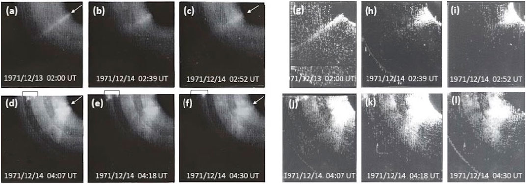
FIGURE 1. Panels (a) through (f): Sequence of images obtained with the Naval Research Laboratory Experiment on OSO-7 on 13-14 December 1971, showing the first evidence of mass transiting through the corona. Panels (g) through (l): Same sequence with a pre-event image subtracted from each image to highlight the evolution of the coronal transient. A preexisting streamer widens and disappears (panels A–C, pointed out by an arrow in the occulter, and G-I). This was followed by the sudden development of a diffuse, enhanced brightness region to the south of the disappearing streamer (panels D-L). Two blobs are seen transiting at the tops of panels (D–L) and pointed to by the black rectangle above panels (D) thru (F). Adapted from NRL Press Release #3-71-1, dated 10 January 1972.
The sequence shows the swelling at the base of a streamer, which loses its top, some brightening and then complete disappearance of the streamer. A sequence of three small, bright patches (blobs) are seen (in panel J, at the top edge of the image, moving outward to the outer left edge of the FOV at a speed less than the escape speed. Exhibiting a slight brightening in an area half way through the FOV, just below the moving blobs and an apparently static diffuse brightening at mid-southern latitudes. The discrete blobs were certainly mass moving outward, but the meaning of the other features and the relation to the other differences, was unknown. A total of nearly 90 min (one orbit) elapsed between the streamer swelling and its disappearance. In hindsight this gap would certainly have been enough time for a streamer blowout CME (Vourlidas and Webb, 2018) as we now know them to have erupted with a broad new streamer forming to the south. The blobs could have been outflow of plasma, which has been seen, recently, very clearly to follow in the wake of a CME (Howard et al., 2022). But at the time, it was realized that this was very unusual and hence a press release was issued in 10 January 19721. All of the data readout modes were present in this sequence: none, quadrant and run-length. Luckily the choice of quadrant was the one that showed the event. The event sequence changed the operational concept to look for brightening/broadening streamers and then to switch to quadrant mode to try to capture it. Unfortunately, OSO-7 only captured 12 events in 20 months or about 0.02/day, so it is safe to say that the new observing strategy was not very successful.
Two homologous CMEs were observed on 11 January 1973 in Hα, white-light and radio from the surface of the Sun out to about 9 R⊙. The WL observations were recorded by the ground-based K-coronameter on Mauna Loa (Hansen et al., 1969) below 2 R⊙ and OSO-7 above 3 R⊙. Stewart et al. (1974b,a) interpreted the events as piston-driven shock waves, originating in a coronal enhancement in the lower corona. The leading edge of the first CME was traveling at about 620 km/s (the type II burst indicated an speed of 800–1,200 km/s) and the second CME at 750 km/s (850 km/s). Moving type IV radio bursts were also seen at both events at the maximum brightness locations of the WL images. A calculation of the mass decrease seen in the K-coronameter was consistent with the mass increase seen in the OSO-7.
2.2 Skylab/ATM
The Skylab spacecraft2 was NASA’s first crewed space laboratory. It was where the astronauts lived, exercised and also operated a number of instruments within Skylab including the six solar pointed instruments within the Apollo Telescope Mount (ATM), a large module attached to Skylab. As shown in Table 1, the launch of the Skylab occurred on 14 May 1973, followed by three crewed mission phases operated by different astronaut crews each with different astronauts, labeled in Table 1 as Skylab 1, 2 and 3. The durations of each crewed mission were 28 days (≈1 solar rotation), 59 days (≈2 solar rotations) and 84 days (≈3 solar rotations), respectively. There was a high degree of observation planning to optimize the science, called Joint Observing Programs (JOPs). The JOPs were developed by the instrument teams who each had a group of scientists in residence during the crewed operations. The National Oceanographic and Atmospheric Administration (NOAA) coordinated their usual space- and ground-based solar data and helped develop the plans of the JOPs. To support the planning process, OSO-7 images were faxed down to the NOAA team.
The crewed missions enabled a unique capability–modifying the observing program while an event was in progress. This was quite effective for a number of the ATM instruments. Between the crewed missions, the coronagraph (described in MacQueen, 1974) data were obtained at a 6-12 h cadence, not enough to capture fast CMEs, but certainly sufficient to capture the large-scale structure of the corona. Briefly, the field of view the telescope is from 1.5 to 6 R⊙ with an 8 arc sec spatial resolution and the detector is film during the crewed phases and a vidicon detector between the crewed phases. The initial results were reported by MacQueen et al. (1976). Figure 2 displays an image from the Skylab coronagraph (Gosling et al., 1974) taken on 10 August 1973, showing a CME in progress. The shape of the structure is similar to the form of what we now know as a magnetic flux rope CME (see Sections 4.3; 5.3).
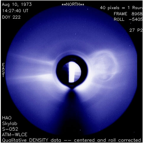
FIGURE 2. A single image of a coronal transient observed by the WLC onboard the Skylab showing a discrete structure on the west limb. We recognize this structure as CME-like (much more so than the one observed by OSO-7). Credit: High Altitude Observatory, National Center for Atmospheric Research, Boulder, Colorado.
The large-scale structure of the solar corona during the 7-month period of Skylab observations was a little unusual. It consisted of two large, strong coronal holes (CHs) at the north and south poles and a rather large low-latitude CH with a CH lane connecting the low latitude CH with the northern polar CH. One side of the Sun was dominated by the large CH while the other side was active and generating CMEs. Solar rotation would then bring these two sides into Skylab coronagraph view, effectively creating a mini-solar cycle in each solar rotation.
2.3 CME science highlights from generation 1
1. The observation of mass leaving the Sun was recognized as an important and regularly occurring solar event. The kinetic energy was estimated as greater than the radiated energy released by a flare and would have a significant effect at Earth. There were events seen in association with other solar phenomena, erupting prominences, flares, radio emission.
2. The occurrence of two homologous events, seen in Hα and radio (Type II and moving IV), showed the timing of the events appropriately aligned (Stewart et al., 1974b; a). An association between the radio observations and the white-light features could be established: the Type II wave was traveling faster than the leading edge of the CME, while the moving Type IV emission was traveling at the position of the maximum brightness of the CME. The estimates of the mass loss in the low corona were consistent with the mass increase in the outer corona.
3. OSO-7 recorded 12 events in 20 months (Koomen et al., 1974), and Skylab recorded 110 in 7 months (227 days) (MacQueen, 1980). Using the definition that a transient is a rapid change (a few tens of minutes) in apparent coronal structure, Skylab observed 115 transients in the 227 days of observations and 77 were definite mass ejections (Munro et al., 1979). Of the remaining 38 events, 26 were changes in the large-scale corona, 4 were possible CMEs, and 8 were questionable. We now know that CMEs are related to large-scale re-arrangements. With the large variation of sunspot number during Skylab, Hildner et al. (1976) was able to see a good correlation (r = +0.67) of the daily frequency of CMEs with sunspot number and also with the Ca II place index (area × brightness). The Skylab rate was about 0.5 CMEs/day, with a strong dependence on heliographic longitude. The fit showed that CMEs were still occurring with a zero sunspot number (more on this in the next-generation discussion). These relationships indicated that the events occurred more often above strong field regions, which also implied that the driving force expelling the mass was magnetic.
4. Gosling et al. (1976) analyzed 38 Skylab CMEs for their speeds and whether they were associated with eruptive prominences (16), flares (11) and radio Type II or IV events (14). The speeds ranged from 100 km/s to 1,200 km/s, with the most probable speeds for all events being about 470 km/s. The flare and Type II/IV associated events had similar speeds, which were about twice as fast as the eruptive prominence associated events. Seven of the events showed accelerations out to the outer limit of the FOV, 5 R⊙. All but one had similar accelerations, resulting in a 200 km/s increase in their speeds during their transport through the FOV. Since none of the events were decelerating, they were not ballistic ejections and there must be a driving force, to, at least, match the gravitational force.
5. Munro et al. (1979) gave a summary of the associations of the Skylab CMEs with other solar phenomena. More mass ejection events (70%) were associated with erupting prominences or disappearing filaments than any other phenomenon. All prominences seen above 0.3 R⊙ from the solar limb were associated with a CME. Of those events most were not associated with a solar flare. The next most frequent association (40%) was with flares, of which 1/2 were with eruptive events. About 1/3 of all events had associated a metric event (Type II or IV) or an X-ray event (Long Duration event, LDE, or a Gradual Rise and Fall event, GRF).
6. The loop-like structure was the most common form seen (about 1/3 of all events), but injections into streamers and amorphous clouds were also seen (Munro et al., 1979).
7. A variety of models were developed, but they generally consisted of a single loop, a manifestation of the flare process or some instability of the magnetic field (e.g., Heyvaerts, 1974; Uchida, 1974; Anzer, 1978; Steinolfson et al., 1978; Hood and Priest, 1979).
3 Generation 2 missions - 1980s
3.1 P78-1/solwind
In late 1973/early 1974, Donald Michels (at the U. S. Naval Research Laboratory) had the idea of flying the OSO-7 flight spare instrument configuration of the WLC and XUV telescopes, with some modifications, on the U.S. Department of Defense (DoD) Space Test Program, which was administered by the U.S. Air Force. The mission received the name Solwind. This proposal process was different from the usual process of responding to NASA’s release of an Announcement of Opportunity (to propose), which is the way almost all of the projects described here have been initiated.
The significant modification for the Solwind mission was the increase of the telemetry rate of the instruments by 10×, i.e., from 200 bits/s to 2000 bits/s. This would involve modifying the WLC electronics package to increase the SEC Vidicon detector readout rate and replace the photomultiplier assembly on the XUV package to use an imaging CCD detector with a microchannel plate (MCP) to convert the UV light into visible photons for the CCD. The only other planned modification was to decrease the inner FOV of the WLC from 3 R⊙ to 2.5 R⊙. The pixel resolution was the same as the OSO-7 coronagraph - 1.25 arcmin/pixel. During the course of the electronics box checkout, several functions had failed due to aging and so they had to be replaced. Other than these modifications, the specifications were the same as for the OSO-7 instrumentation (Koomen et al., 1975). The P78-1 spacecraft was also the OSO-7 flight spare, which had been modified to accommodate the new instrumentation and to provide a larger solar array. The launch of the P78-1 spacecraft occurred on 24 February 1979 into a sun-synchronous noon-midnight orbit, which still had a day/night cycle. In May 1985, the last of the three tape recorders failed, which meant that data could only be taken in real-time, while the spacecraft was in contact with a ground station. In addition the batteries were failing, creating power outages due to under voltage. The mission ended on 13 September 1985, when it was used as the target of an Anti-Satellite weapon test3.
3.2 SMM coronagraph/polarimeter
The Solar Maximum Mission (SMM) was launched on 14 February 1980 carrying a WLC, the Coronagraph/Polarimeter (C/P), as one of six instruments to study the Sun. The C/P is described in detail by MacQueen et al. (1980). Briefly, it is a follow-on to the Skylab and balloon coronagraphs discussed earlier. It was an externally-occulted coronagraph with 3 external disks and an SEC Vidicon as the detector. The FOV covered coronal heights between 1.5 and 6 R⊙, but a mirror would project a quadrant of the full field onto the detector. There were a total of six quadrants that could be used. A polarizer wheel with 3 linear polarizers enabled a polarization analysis of the signal to help distinguish between the scattering of electrons (K-corona) or dust (F-corona). The pixel resolution was 6.4 arc sec/pixel. A number of spectral filters were included to obtain images in the Fe XIV green line and H-α as well as various broad band colors.
The C/P operated from 1980 to 17 November 1989 with an interruption from September 1980 to April 1984, due to several hardware failures. About 1,300 CMEs were observed during the SMM operating period (Hundhausen, 1993a).
3.3 CME science highlights from generation 2
1. The combination of SMM and P78-1 covered nearly a solar cycle with good coverage, resulting in very good characterizations of CMEs, their associations and kinematics.
2. The view of a CME heading straight at the observer is shown in Figure 3. It was called a halo (Howard et al., 1982) due to the annulus of brightness surrounding the occulting disk. This was the first observation of a CME headed toward Earth. This observation demonstrated that the CME was not a planar structure but had a 3D shape. One outstanding issue at the time was whether the observed feature corresponded to the CME itself or to the associated shock. This CME went on to cause a geomagnetic storm, indicating the potential of such observations for forecasting geospace disturbances.
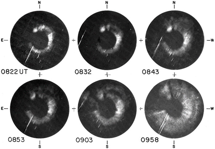
FIGURE 3. Sequence of images of a halo CME, observed by the Solwind WLC on 27 November 1979, showing enhanced emission surrounding the occulting disk. This is indicative of a CME propagating along the Sun-observer line either toward or away from the observer. In this case the CME was coming toward the observer. Adapted from Howard et al. (1982).
3. The associations seen in Gen 1 were confirmed with Gen 2 with excellent statistics now due to the increased number of CMEs observed. Sheeley et al. (1983) found that the longer the duration of the soft X-ray event, the higher the likelihood of a CME (durations ≥6 h were 100% likely to have a CME). For 50 prompt proton events between April 1979 and February 1982 for which Solwind data were available, Kahler et al. (1984) found that there were 26 associated H alpha flares, and of those there were 26 CME events, indicating a strong but not perfect correlation. Cliver et al. (1983) found that a series of CMEs and flares from 45° range of Carrington longitudes occurred during mid-1982. Due to solar rotation the CMEs and shocks from those events were spread out across many ecliptic longitudes and generated an outward propagating shell that surrounded the Sun. This produced the observed azimuthal symmetry of the cosmic ray modulation in the Pioneer 11 and Pioneer 10 (McNutt et al., 1996, see also https://www.nasa.gov/centers/ames/missions/archive/pioneer.html) data. Finally, in a study of CMEs and metric Type II events, Sheeley et al. (1984) found that shocks without CMEs have a relatively impulsive origin and may die out sooner that CME piston-driven shocks, and either some fast CMEs do not reach shock-producing super-Alfvénic speeds within the low corona where the metric emission is formed.
4. The archetypal form of a CME was identified as a three-part structure (Illing and Hundhausen, 1985). Namely, a bright front followed by a dimmer region and a bright core behind (see Figure 4; the core is prominence material, clearly shown in the lower right frame, which is not always visible). Later on, this structure became identified as a magnetic flux rope (MFR; Chen et al., 1997).
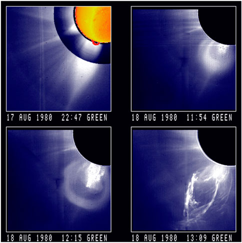
FIGURE 4. The three-part CME observed by C/P on 18 August 1980. The streamer in the upper left panel is seen to broaden and then disappears as the CME starts outward. In the lower left the 3 parts are clearly visible. Adapted from Illing and Hundhausen (1985).
5. Howard et al. (1985) performed statistical analysis of nearly 1,000 CMEs from 1979 to 1981. Several structural forms were added to those seen by Generation 1. The lower resolution and sensitivity of Solwind compared to C/P resulted in different apparent forms being identified. Figure 5 shows the 9 forms that were identified by Solwind. The loop and double spike are most likely the same. The Solwind and C/P data for a few events were checked and the loop tops that were present in the C/P images were missing from the Solwind data. The curved front, halo, and multiple spike types could be the same structure, just seen from different perspectives. The single spike is an ejection along a streamer. A multiple spike might be multiple events. A fan shows no internal structure. This will be discussed in Section 4. The statistics of the various structural forms are given in Table 2. Although this table is from Solwind, the C/P statistics (Hundhausen, 1993b; Hundhausen et al., 1994) were consistent.
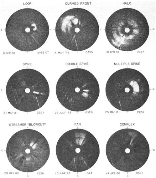
FIGURE 5. Examples of the various categories of CME shapes that were used in the Solwind analyses. See text for further description. Adapted from Howard et al. (1985).
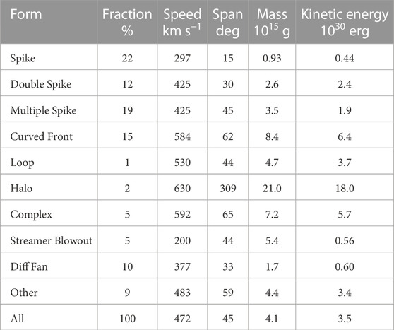
TABLE 2. Average Properties of Coronal Mass Ejections 1979-1981 (From the Solwind mission data.) Examples of the various CME types are shown in Figure 5.
6. The association of CMEs to interplanetary (IP) shocks and IP magnetic clouds was clearly established. Sheeley et al. (1985) showed that about 72% of the shocks seen at the Helios 1 (Marsch and Schwenn, 1990) spacecraft during the interval 1979-82 were definitely associated with low latitude CMEs. Another 27% were possibly associated with a CME but there were issues that made them less certain. This study was so successful due to the orientation of the Helios 1 orbits during these years, which was approximately 90° from the Sun-Earth line. The Helios 1 was in an approximately 6-month orbit about the Sun with a 0.3 au perihelion and 1.0 au aphelion. Thus, it would spend most of the orbit near the aphelion over one limb and then in a few weeks go through perihelion to the other limb. Spending most of its time over a limb made it ideal for coronagraph collaborations. As an extension to the shock study, Woo et al. (1985) used the Doppler scintillations obtained from the Jet Propulsion Laboratory tracking of the various planetary probes. With the timing of the scintillations he was able to track the passage of the shocks from the Sun to Helios and found that the shocks decelerated more the faster they were and not at all if slow enough.
7. Howard et al. (1986) plotted the yearly averages of the number of Solwind CMEs/day against the Solar sunspot Number (SSN) for years 1979-1982 and 1984-85 and found that the slope was the same as Hildner’s Skylab rate but the absolute rate was 0.1 CME/day lower. Webb and Howard (1994) extended the study to include data from all four instruments in Generations 1 and 2 showing correlations of frequency with SSN, Metric II and flares by year.
8. The upper panel of Figure 6 displays the flare latitudes as recorded in data from the NOAA World Data Center A in Boulder, Colorado. The bottom panel shows the latitude of the CME central axis (as observed with the C/P instrument onboard the SMM), indicating that it follows the solar cycle (Hundhausen, 1993b). At the maximum of the solar cycle, the central axis could occur at any latitude, but as the solar cycle approached minimum, the range of latitudes narrowed, until at minimum it was narrowly distributed around the heliographic equator. This was partly due to the deflection of the eruption toward the solar magnetic equator. The two types of events follow the solar cycle, but the flare latitudes are restricted to ≈ ± 30°, much less than the extent of the central CME latitudes. This was one of the arguments made by Gosling (1993, 1994) in his discussion of the Solar Flare Myth.
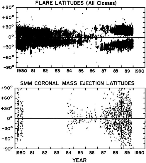
FIGURE 6. Solar latitudes of solar flares (from the NOAA World Data Center A in Boulder, Colorado) and of SMM C/P CMEs from 1980 to 1990. No SMM CMEs were observed from 1991 to 1994. See the text for further information. Adapted from Hundhausen (1993b).
9. Jackson and Howard (1993) plotted the number of Solwind CMEs with a given mass against that mass on a log-linear scale, and found that the mass distribution was linear over more than a decade of CME masses. This allowed for an easy determination of the total mass ejected into the solar wind in the form of CMEs. They found that approximately 16% of the solar wind at solar maximum can be comprised of CME mass. Furthermore, there is a fall off at the low-mass end and no indication that an increase exists in the number of low-mass CMEs. The fall off at low mass end could be due to the detection limit imposed by the detector or the low speed limit of 50 km/s for distinguishing a CME from outflow.
10. Streamer blowout (SBO) events were identified as a unique event (Howard et al., 1985) and will be discussed more fully in Generation 3 results. The streamer blowout (SBO) event refers to those events in which the large-scale magnetic field pattern was altered and the post-CME streamer appeared at a different location, in contrast to when the large-scale pattern did not change and the streamer reappeared at the same location. That is, a CME often occurred in the location of a streamer, which then disappeared. If the streamer reappeared at a different latitude, this is the indication that the large-scale pattern was altered, and the streamer eruption was due to that alteration. If the streamer reappeared at the same latitude, then the large-scale pattern was not altered. It was speculated that the mechanisms for these two different events are different (Howard et al., 1986; Vourlidas and Webb, 2018). It was also observed that the frequency of SBO events did not increase throughout the solar activity cycle, but was fairly constant (Howard et al., 1986).
11. CME modeling seemed to follow on to the previous ideas of modeling identified in the Generation 1 results.
4 Generation 3 missions - 1990s
4.1 Spartan 201-1 white-light coronagraph
Following the launch of the first space shuttle (Naugle, 1973), a new concept was developed (Cruddace et al., 1985) to extend the short flight time of rockets, about 8 min of flight, to a few days. The concept was to carry rocket-like instruments in the bay of the shuttle and then deploy them in space, allowing them to orbit near the shuttle and finally retrieve the instrument before the end of the sortie mission. Observations would be independent from the shuttle.
The Spartan 201-1 mission was one of such programs, which consisted of a WLC (Fisher and Guhathakurta, 1994) and an Ultraviolet Spectrometer (Kohl et al., 1994). The mission was launched on the Discovery shuttle on 7 April 1993. This WLC was built with a single serrated external occulter (Fort et al., 1978) and a Charged Coupled Device (CCD) for the detector (Blouke et al., 1981). The cadence of image acquisition was very good, and it was able to acquire simultaneous observations of a CME in WL and Ly-α.
4.2 Large Angle and Spectrometric coronagraph (LASCO) and extreme-ultraviolet imaging telescope (EIT)
The European Space Agency’s (ESA) Solar and Heliospheric Observatory (SOHO) (Domingo et al., 1995) was launched on 2 December 1995 from Cape Canavaral, Florida. It was an ESA mission, with extensive NASA participation in a good partnership. The spacecraft was sent into orbit about the L1 Lagrangian point, a point about 1.5 × 10⁶ km sunward from Earth, where the gravitational forces of the Sun and Earth balance the centripetal force required for the spacecraft to move with them. The L1 location was a game changer–it provided continuous solar viewing for the remote sensing imagers and no shadowing from the Earth or magnetosphere for the in-situ instruments.
SOHO was one of the cornerstone missions of ESA that had been under discussion within the scientific community for nearly 20 years. It was designed to be and became a significant solar and heliospheric observatory with a set of 12 instruments to study the Sun, from its interior to the surface, and from the corona out to the solar wind crossing the spacecraft. Designed to work for 2 1/2 years, it is still working. Initially, the instrument teams were in residence at the control center at NASA’s Goddard Space Flight Center (GSFC), but in 2011, the operations concept changed and became virtual. NASA had then launched the Solar Dynamics Observatory on 11 February 2010 (Pesnell et al., 2012), which replaced some of the SOHO instruments.
The remote sensing instruments in the SOHO payload best suited for the observation and study of CMEs are the Large Angle and Spectrometric COronagraph (LASCO, Brueckner et al., 1995) suite and the Extreme Ultraviolet Imaging Telescope (EIT, Delaboudinière et al., 1995). LASCO consists of three visible light telescopes to image the solar corona from 1.1 R⊙ to 30 R⊙. The telescopes have nested and overlapping FOVs: C1 from 1.1 to 3 R⊙, C2 from 2 to 6 R⊙ and C3 from 3.7 to 30 R⊙. EIT is a normal-incidence ultraviolet telescope with a FOV of ±1.4 R⊙ to image the solar disk and corona at four UV wavelengths. The combination of EIT and LASCO allowed for the continuous viewing of the solar corona from the disk out to beyond the Alfvén critical surface, i.e., where the solar wind separates from the Sun (e.g., Kasper et al., 2021).
C1 is an internally-occulted Lyot mirror coronagraph with a Fabry-Perot interferometer enabling scans around the coronal lines of Fe XIV, Fe X, Ca XV, Na I, and H-alpha, as well as a broad band continuum. C1 failed at the SOHO spacecraft loss of pointing in 1998, when the instruments were powered off and the LASCO temperature dropped below −90 C, well below the design limit of −40 C.
C2 and C3 are externally-occulted Lyot WLCs, similar to what has flown previously. Both have polarization wheels to determine the state of polarization of the coronal signal, to create the pB signal, which greatly enhances the relative contribution of the K-corona component, and hence help separate the F- and K-coronae.
The EIT uses four multi-layer thin filters to select the EUV emission in four wavelengths–Fe IX (17.1 nm), Fe XII (19.5 nm), Fe XV (28.4 nm) and He II (30.4 nm), which provides temperature diagnostics in the range from 6 × 10⁴ K to 3 × 10⁶ K.
The detectors for LASCO and EIT are 1Kx1K charge coupled devices (CCD; Blouke et al., 1981; Janesick and Blouke, 1995) manufactured from the same lots. The LASCO CCDs were frontside detectors, meaning that the light was passing through the electronic structures deposited on the silicon wafer. Those structures would absorb the UV radiation. Therefore, the EIT detector was back-thinned to allow the UV radiation to penetrate into the collecting volume toward the front surface. The pixel size of the LASCO detectors are 5.6″, 11.4″, 56.0″, for C1, C2, C3, respectively; and of the EIT detector 2.6”.
Among the LASCO’s technical improvements are a very large FOV, both closer to the Sun and further out than previous coronagraphs, and the CCD detector with a much greater dynamic range than the Vidicons and film detectors. The location of the SOHO spacecraft allowed for an uninterrupted continuous solar viewing.
4.3 CME science highlights from generation 3
1. First simultaneous observations of a CME in Lyα and WL (Hassler et al., 1994).
2. The initiation in the low corona of a small CME was captured with EIT and LASCO/C1 (Dere et al., 1997). In a sequence of images on 23 December 1996, in EIT 19.5nm, a prominence erupts followed by a dark cavity forming behind it. The cavity grows and then expands laterally. The C1 Fe XIV 530.3 nm green line image apparently sees the same cavity a little further out and closer to the equator than the original EIT images. In LASCO/C2 it became a diffuse brightness enhancement along a streamer.
3. Thompson et al. (1999) showed the first example of an EUV wave (expanding depletion region) in conjunction with a large CME in EIT and LASCO/C2 (event on 7 April 1997). Many such examples have been seen since then (Long et al., 2017, and references therein). They interpreted the expanding structure as a large EUV wave (and possibly the EUV counterpart of an H-α Moreton wave; Moreton, 1961; Athay and Moreton, 1961), which expanded and ultimately filled the visible disk.
4. Figure 7 displays composite frames of a CME observed on 9 September 1997 by the HAO Mark III K-coronameter (Fisher et al., 1981) and LASCO/C2 exhibiting a clear 3-part structure. The K-coronameter images below 2.2 R⊙ and the LASCO/C2 above. Chen et al. (2000) identified this CME as having the shape of the magnetic flux rope, similar to an earlier event on 13 April 1997 (Chen et al., 1997). The letters A, B and C in Figure 7 point, respectively, to the bright circular frontal rim, to a bright ray structure that persists, and to the extended emission to the south of the frontal rim. The lower right panel is a composite of MK3 and LASCO/C2 images at the time corresponding to the upper left panel, in which a pre-event image has been subtracted off, revealing just the bright front. Note that the CME has the 3-part structure, but perhaps it should be extended to be a 5-part structure, since the dim region surrounds the core (i.e., the prominence material) and the bright front completely circles the dark core (Vourlidas et al., 2013). The view point is slightly off the axis of the MFR, revealing emission extending below the southern edge (C). This was interpreted as depth of the along the LOS, again pointing out the 3D nature of the CME.
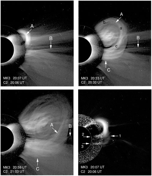
FIGURE 7. Combined images of the Mk3 K-coronameter and LASCO/C2 on 9 September 1997 showing the manifestation of a magnetic flux rope. See text for further description. Adapted from Figure 2 in Chen et al. (2000).
5. Webb et al. (2000) found that all six halo CMEs observed by LASCO between December 1996-June 1997, were associated with shocks, magnetic clouds, and moderate geomagnetic storms at Earth 3-5 days later. This implied that magnetic clouds are an interplanetary counterpart of CMEs. In addition most of the storms in this interval were driven by strong, sustained southward fields either in the magnetic clouds, in the post-shock region, or both. Thus, the relevance of halo CME for space weather was acknowledged.
6. As part of the Coordinated Data Analysis Workshops (CDAW), a catalog of all of the CMEs observed by LASCO have been manually identified and their properties determined (Yashiro et al., 2004; Gopalswamy et al., 2009) and made publicly available4. To date over 33,000 CMEs have been recorded! Figure 8 is a screenshot of the CMEs identified for 1 May 2023. Similarly, a catalog of Halo CMEs (Gopalswamy et al., 2010) has been generated separately and is also publicly available5.
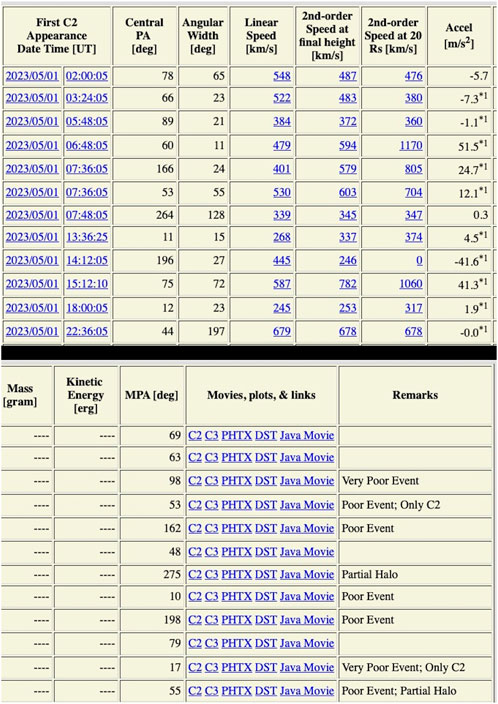
FIGURE 8. Display of the output from the CDAW LASCO CME catalog for the CMEs identified for 1 May 2023. The display was split in half to fit on the page.
7. The effort to manually identify and measure over 33,000 CMEs is quite a challenge, which was an impetus for finding an automatic algorithm. Berghmans (2002) developed the first concept for an automatic detection algorithm of CME events in the FOV of white-light coronagraphs, the so-called Cactus algorithm (Computer Aided CME Tracking); and Berghmans et al. (2002) first applied it to CME events observed by LASCO. This was followed with an update by Robbrecht and Berghmans (2004). Olmedo et al. (2008) followed this with a slightly different algorithm called Solar Eruptive Event Detection System (SEEDS). Both the CACTUS6 and SEEDS7 lists are also available publicly. All of the catalogs continue to be updated.
8. With the identification of the MFR, a tool to empirically fit the CMEs to help define their boundaries and axes was needed. Thernisien et al. (2006) developed such a tool, which was applied to the 20 December 2001 CME. For this event, they were able to fit the density profile of the leading edge very well, giving a maximum density of 2.9 105 e− cm−3. The model was called the Graduated Cylindrical Shell (GCS), or sometimes, the croissant model. There can be a difficulty in forming a unique fit from a single viewpoint. The GCS model was also originally applied (Thernisien et al., 2006) to the four CMEs identified by Cremades and Bothmer (2004), which appeared in the four quadrants of LASCO. The model fits explained their different appearance in the four quadrants. Later on, Thernisien (2011) applied the GCS model for the three-dimensional reconstruction of CMEs.
9. Vourlidas et al. (2010, 2011) analyzed 7820 LASCO CME events and found two populations of events, equally frequent. Figure 9 shows two scatter plots displaying the mass evolution with height of all 7,820 CMEs. The distinct behavior of the two classes is obvious. As seen in the left panel, for one type of CME, the mass increases gradually from the beginning to the end of the FOV, reaching about 1016 g. The mass is computed assuming that all the mass is on the Thomson Surface (TS; Vourlidas and Howard, 2006). The right plot gives the average electron density of about 3.55 ± 0.29 e−cm−3. The other type of CME shows a rapid increases in mass, almost reaching 1016 g, but seem to disappear, as they are not seen beyond ≈ 8R⊙. This second class of CMEs are called pseudo-CMEs. In the right panel, the slow decline of the mass volume density toward the outer FOV is consistent with the reduced S/N at these heights and them leaving the FOV. They found no evidence of material pileup.
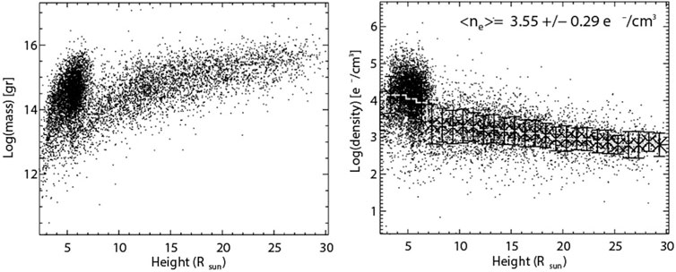
FIGURE 9. Scatter plots showing the height dependence of the logarithm of the total CME mass (left panel) and the CME volume density (in e− cm−3; right panel). For the right panel plot, a histogram with 1R⊙ bins is calculated and the average density (asterisks) and standard deviation (error bars) in each bin are over-plotted. The density is derived assuming an LOS depth equal to the projected width. Adapted from Vourlidas et al. (2010, 2011).
10. Petrie (2015) found an increase in the LASCO CME rate at the time of the solar polar field reversal. In the three LASCO CME databases SEEDS, CACTus, and CDAW, a statistically significant increase in the rate of CME detections with angular widths larger than 30° per sunspot number was found for cycle 24 compared to cycle 23. The increase in the CME rate began in 2004 after the polar field reversal. At nearly the same time, the interplanetary magnetic field (IMF) decreased by ≈ 30%. This behavior is consistent with three previous findings by Gopalswamy. In the last cycle Gopalswamy et al. (2003) found a cessation in high latitude CMEs at the polarity reversal. In the current cycle (24) Gopalswamy et al. (2014) found an anomalous increase in CME widths at the polarity reversal along with a 40% decrease in heliospheric pressure. Finally, Gopalswamy et al. (2015) linked enhanced halo CME detections to increased CME expansion in a heliosphere of decreased total magnetic + plasma pressure. The appearance of Halos is a geometric effect, but they found that the location of the origination longitude had increased to ±60°, which is twice what it was in cycle 23.
11. Vourlidas and Webb (2018) performed a detailed analysis of the SBO type of events from LASCO, using 909 events compared to the 50 ones detected by Solwind. The top panel of Figure 10 shows the typical development of an SBO event: slow swelling of a streamer for a day or more, a three-part CME emerging slowly and accelerating, followed by plasma outflow lasting for hours, leaving behind a depleted streamer. The CME transits out of the LASCO/C2 FOV by 17:30 UT, but the coronal evacuation continues until about 20:48 UT on March 25, making this an approximately 3-day event. The bottom panel of Figure 10 shows the Carrington map for the West Limb at 2.5 R⊙ for data from 30 October 2008 to 27 November 2008. Note that time increases from right to left. The map shows a new streamer reforming at a different position angle after both SBOs, implying a change in the global magnetic field configuration.
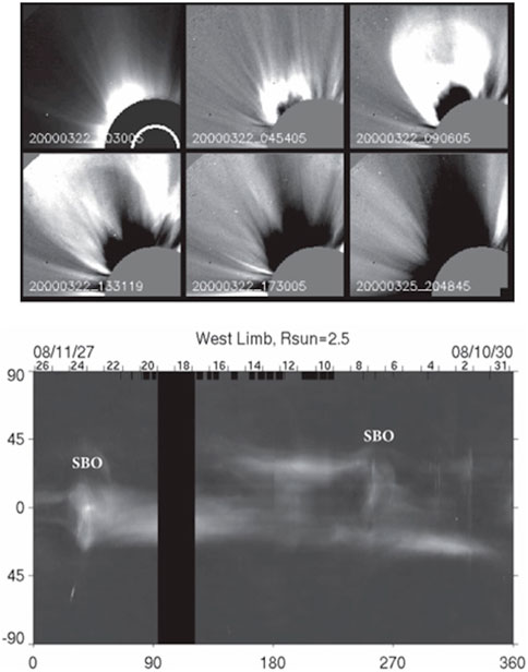
FIGURE 10. Top panel: Example of an SBO event recorded by LASCO/C2 on 22 March 2000. The image at 00:30 UT is the pre-event image, and all subsequent images are differences from that image. Bottom panel: Examples of SBO CME events in LASCO Carrington maps. Time runs from right to left. The two SBO events both show the formation of the streamer thereafter at a different latitude. Adapted from Vourlidas and Webb (2018).
5 Generation 4 missions - 2000s
5.1 Coriolis/Solar Mass Ejection Imager (SMEI)
The Coriolis spacecraft, a DoD Space Test Program mission, was launched on 6 January 2003 from Vandenburg AFB, CA, into a sun-synchronous circular orbit in the dawn-dusk plane about Earth. It carried two instruments–a heliospheric imaging telescope (the Solar Mass Ejection Imager or SMEI Eyles et al., 2003; Jackson et al., 2004) and a multi-frequency polarimetric radiometer, WINDSAT (https://www.remss.com/missions/windsat), to measure sea surface wind vectors.
The SMEI instrument consisted of three identical heliospheric imagers mounted at different viewing angles to the Sun, giving nearly a 4π coverage of the heliosphere, excluding a 18° circle around the Sun. Each telescope had a 60° x 3° FOV. The rotating spacecraft allowed the build-up of 3° strips every 4 s, the exposure time. The passband was 450-950 nm, defined by the response window of the CCD detector for a quantum efficiency above 10%. The CCDs had 1,242 × 576 pixels.
5.2 STEREO SECCHI
The twin Solar Terrestrial Relationships Observatory (STEREO) spacecraft Kaiser et al. (2008) were launched 25 October 2006 from Cape Canaveral AFB, FL. They were nearly identical spacecraft, stacked on top of each other at launch, separated post-launch for eccentric orbits about the moon. At different times, they were sent into a close flyby of the moon to escape Earth’s gravity into orbits about the Sun near 1 AU. The orbit of STEREO-A orbit is slightly inside Earth’s orbit and hence it leads Earth. On the other hand, STEREO-B’s orbit is slightly beyond Earth’s orbit and hence it trails Earth. Both spacecraft drift away from Earth at a rate of about 22.5° per year.
Planned to last 2.5 years, both spacecraft worked well until October, 2014, when communication with STEREO-B was lost, before the spacecraft would have lost communication with Earth due to the superior conjunction. It was not recovered for normal operations. The STEREO-A spacecraft passed through superior conjunction unscathed, and has continued to work well to the present day.
The SECCHI suite of 5 telescopes (Howard et al., 2008) were nearly identical on the two spacecraft, providing a view of the region of space from the solar UV surface to 1 au, using a series of nested FOVs. They all used 2 K × 2 K CCDs as the detectors. The Extreme Ultra-Violet Imager (EUVI; Wülser et al., 2007), was a similar instrument to the SOHO/EIT instrument with the same narrow band channels. It has a ±1.7R⊙ FOV and 1.6″ pixels. COR1 is an internally occulted refractive Lyot coronagraph with an annular FOV from 1.4 to 4 R⊙ and 3.75″ pixels and with a passband of ±25 nm at 656 nm. COR2 is an externally occulted Lyot coronagraph with an annular FOV of 2.5-16 R⊙ and 14.7″ pixels and with a passband of 650-750 nm. Both COR1 and COR2 had linear polarizing filters to perform polarization analyses. The HI1 and HI2 telescopes (Eyles et al., 2009) were in a separate package on the Sun-Earth side of the STEREO spacecraft. HI1 is a heliospheric imager with a linear occulter at 4° from Sun center, with a 20° FOV, equivalent to 15 to 90 R⊙, 70” pixels (with 2 × 2 pixel sums) and bandpass of 640-730 nm. The HI2 is also a heliospheric imager with a linear occulter at 18.7° from Sun center, with a 70° FOV, equivalent to 70 to 332 R⊙, 4’ pixels (with 2 × 2 pixel sums) and a bandpass of 400-1,000 nm.
5.3 CME science highlights from generation 4
Many very good CME-related papers have appeared using the Gen 4 instrumentation but we have restricted this list to what we considered to have provided a significant first view into new phenomena.
1. Gopalswamy et al. (2001) discovered the cannibal event where a faster CME overtakes another. This was not observed optically, but from radio emission. The radio signature is in the form of intense continuum-like radio emission following an interplanetary type II burst. Other occurrences of this radio signature were noted in the October-November 2003 storms (Gopalswamy et al., 2004).
2. Webb et al. (2006) gave a summary (including a catalog of all the events) of the SMEI observations of CMEs from this first-of-its-kind instrument. In the first 1.5 years of operaton, SMEI observed 139 CMEs and at least 30 traveled to at least 1 AU, causing geomagnetic storms. Those CMEs were seen as halos in LASCO. The speeds were between 51 and 1,611 km/s with a mean of 473 km/s using the Point P approximation to convert elongation angles into radial distances (Howard et al., 2006). From a comparison with the LASCO CME occurrence rates, SMEI was seeing the brighter, more massive CMEs.
3. Thernisien et al. (2009) applied the GCS fitting to a number of CMEs observed from the two viewpoints provided by STEREO-A and STEREO-B. They found that the two viewpoints improved the error of the fitting. They find a precision on the longitude and latitude to be a maximum of ±17° and ±4°, respectively. But the precision on the flux rope orientation and length to be almost one order of magnitude larger. But if the CME axis is in the same plane as the observers, the solution is not unique.
4. Robbrecht et al. (2009) presented the first evidence of a CME without any low coronal signatures, known as a stealth CME. While this may have been seen in the past, the single view from Earth could not definitively rule out other possibilities, but they were by using STEREO data.
5. Cheng et al. (2012) showed a very good set of observations of the initiation of a CME made by the Atmospheric Imaging Assembly (AIA) telescope (Lemen et al., 2012) onboard the SDO mission, combined with the SECCHI EUVI and COR1 on the STEREO A and B spacecraft. Using images from all the telescopes they showed the relation of the EUV emission to the WL, and tracked the extension of a CME shock from the front of the WL CME as it deflected streamers on either side of the CME.
6. Shen et al. (2013) found a case of two CMEs being launched from the same active region, only ≈2 min apart. The event occurred on 17 May 2012 and they used data from LASCO, SECCHI/COR1A, and SECCHI/COR2B, as well as other observatories. Both CMEs were fast (1,258 km/s and 1,559 km/s) and generated complex radio emissions, with multiple type II episodes, high energy SEPs. The pre-eruption magnetic field configuration as measured by the Heliospheric Magnetic Imager (HMI; Scherrer et al., 2006) on board the SDO mission consisted of a twisted flux-tube structure.
7. Wang (2015) reported on CMEs from pseudostreamers, which do not consist of magnetic flux ropes and do not transit to very high heights before the material drains back. Could these be the source of at least some of the failed CMEs described by Vourlidas et al. (2010)?
8. The extensive research on CMEs and their impact on the Earth’s magnetosphere was the impetus for the National Space and Technology Council (NSTC) to establish the National Space Weather Strategy and Action Plan, which were released by the White House in 2015 (Jonas and McCarron, 2016; Murtagh, 2016)8. SECCHI demonstrated how useful a viewpoint away from the Sun-Earth line is for SW monitoring and for understanding the CME phenomena. A viewpoint out of the ecliptic would help resolve ambiguities, for scientific purposes, if not for forecasting.
9. Vourlidas et al. (2017) compiled a very extensive CME catalog based on the simultaneous COR2 STEREO-A and-B observations. It showed that the viewing location relative to the CME makes quite a difference (Balmaceda et al., 2018).
6 Generation 5 missions - 2010s
On 12 August 2018 the NASA Parker Solar Probe (PSP) (Fox et al., 2016) was launched from Cape Canaveral AFB, FL on an ambitious mission to orbit the Sun with an expected final perihelion of 9.98 R⊙ from Sun center on 24 December 2024, through a series of seven gravity assists from close flybys of Venus (VGA). To date five VGAs have been performed, which have lowered the perihelion to 13.28 R⊙ and the data have been remarkable.
The Wide Field Imager for Solar Probe instrument (WISPR) (Vourlidas et al., 2016) is one of four instruments on PSP and the only remote sensing instrument. It consists of two heliospheric imagers (similar in concept to the STEREO/SECCHI HIs) with a total FOV of about 95° radial and 45° transverse looking in the direction of the spacecraft motion. The detectors are Advanced Pixel Sensors (APS) of 2048 × 1920 pixels2. The data are collected when the spacecraft is within 0.5 AU of the Sun.
On 9 February 2020, the Solar Orbiter (SolO) mission (Müller et al., 2020; García Marirrodriga et al., 2021) was launched from Cape Canaveral AFB, Florida, also on an ambitious mission to fly outside of the ecliptic plane, using gravity assists from Venus and Earth (EGA). To date it has executed 2 VGAs and 1 EGA and has a perihelion distance of about 0.29 AU. SolO carries 6 remote sensing and 4 in-situ instruments. SolO perihelion is currently at 0.3 AU in the ecliptic plane but after the fourth VGA in February, 2025, the orbit will reach ±15° solar latitude and after the sixth VGA in March 2028 the orbit will reach over ±30° solar latitude.
The Metis instrument (Antonucci et al., 2020; Fineschi et al., 2020) onboard SolO is an ultraviolet and white-light coronagraph. It takes images in the H I Lyman-α spectral line and the WL corona, from which the outflow speed of the solar wind using the Doppler dimming technique can be obtained. The FOV is an annulus from 1.6 R⊙ to 2.9 R⊙.
The Solar and Heliospheric Imager (SoloHI; Howard et al., 2020) onboard SolO is also similar to the STEREO/SECCHI/HIs. It has the same FOV, 40° square, but twice the spatial resolution. The detector (Korendyke et al., 2013) is a mosaic of the same detectors as WISPR, 2048 × 1920 pixels2, arranged in a pinwheel fashion: 2 sides are butted together, thus forming an array of 4 detectors, with each detector rotated 90° from each other; the other two sides have electronic circuitry to control the rows and columns. Thus, in the mosaic, the electronic circuitry is completely around the mosaic.
Both PSP and SolO are providing absolutely unique views of the inner heliosphere, and already adding tremendous insights to the existing and new missions that will be coming along. Here are a few papers that illustrate the potential of these two novel missions.
1. Some papers have compared CMEs detected from different distances close to the Sun (e.g., as observed by SolO/Metis, SolO/SoloHI and/or PSP/WISPR) with CMEs observed at 1 AU by STEREO/SECCHI or SOHO/LASCO exploiting the different perspectives of those instruments. Examples are.
• Hess et al. (2020), who compared PSP/WISPR with SOHO/LASCO and UV images from SDO/AIA;
• Wood et al. (2020) who compared a PSP/WISPR CME with the same one seen by STEREO/SECCHI and SOHO/LASCO, finding that the blob like events at 1 AU started as a small magnetic flux rope in PSP/WISPR;
• Braga and Vourlidas (2021), who compared PSP/WISPR CMEs with SECCHI/HI CMEs, finding that one accelerated between 0.1 and 0.2 AU;
• Braga et al. (2022), who observed a deformation in a PSP/WISPR CME and compared it to the same CME seen in SOHO/LASCO and STEREO/SECCHI; Mierla et al. (2023) who analyzed the morphology, direction of propagation, and 3D properties of 3 erupting prominences observed in the ultraviolet by the SDO/AIA and the Extreme Ultraviolet Imager (EUV; Rochus et al., 2020) on SolO, which preceded 3 CMEs observed by SolO/Metis, STEREO/SECCHI and SOHO/LASCO.
2. The higher resolution resulting from the imaging instruments being close to the Sun can be as high as 20× the 1 AU resolution. This has resulted in the observation of additional structures within the magnetic flux rope and examples of cannibal CMEs–a faster CME overtaking and colliding with a slower one (Howard et al., 2022).
3. The close distance of the observer to the Sun causes the Thomson surface to become smaller so that the distance from the observer to the Thomson surface becomes smaller (Vourlidas et al., 2016). The effect of this is to reduce the volume of space which contributes to the signal, hence improving the contrast between closely spaced structures. Stenborg et al. (2023) showed that the region depleted of material in the wake of big CME events indeed decreases the observed brightness. In particular, they showed that a CME event detected by PSP/WISPR on 5 September 2022 evacuated not only electrons but also dust particles in orbit around the Sun. This is the first direct observation of dust evacuation. The effect has been theoretically postulated (Ragot and Kahler, 2003) but never observed before.
6.1 A brief commentary on CME modeling
Efforts to model CMEs, from their initiation to their formation and propagation to Earth and beyond, have greatly increased since the establishment of space weather programs across the U.S. federal agencies funding research for such science (DOD, NASA, NSF and NOAA) and across the world. Chen (2011), Forbes et al. (2006) and Mikić and Lee (2006) provide extensive reviews of the physics of CMEs and the history of CME modeling. Significant progress has occurred on the problem of CME initiation and energy release since the publications of these reviews. It is now widely accepted that the ejected structure is a magnetic flux rope, as all models seem to predict (e.g., Vourlidas et al., 2013, and referencees therein). However, the fundamental question of how CMEs are initiated remains uncertain (Patsourakos et al., 2020).
Three numerical MHD modeling capabilities dominate CME heliospheric propagation modeling: (1) Block Adaptive Tree Solar-wind Roe Upwind Scheme (BATSRUS) (Manchester et al., 2004), (2) EUropean Heliospheric FORecasting Information Asset (EUHFORIA) (Pomoell and Poedts, 2018), and more recently, (3) Grid Agnostic MHD for Extended Research Applications (Gamera) Zhang et al. (2019).
In addition to the theoretical and MHD models, a numerical hydrodynamic model has been extensively used to propagate CMEs to Earth and beyond (Odstrčil and Pizzo, 1999). Also, ENLIL is currently being used by the NOAA’s Space Weather Prediction Center to help predict the arrival of CMEs at Earth.
In addition to these physics-based approaches, empirical models have been developed to assess CME propagation (Vourlidas et al., 2019, and references therein) or just to determine the shape of an observed CME from one or more viewpoints. The model, developed by Thernisien et al. (2006, 2009); Thernisien (2011), uses the shape of a simple magnetic flux rope to define the electron density structure. A recent model by Weiss et al. (2021, 2022), includes the CME magnetic field in its fitting, and enables a distorted MFR to fit the CME.
7 Conclusion
In this paper, we presented a succinct overview of the significant findings in CME research, from the pioneering research leading to the discovery of mass being ejected from the Sun to the most recent advances in the field. All of the space-based missions with at least a WLC onboard that produced some data have been included. We have described these missions in chronological order, conveniently grouping them into generations. Technological advances and knowledge acquired allowed for each new generation to produce significant advances. Next, we summarize the scientific and technological enhancements that led to the actual state of knowledge.
In Generation 2, the most significant advance, over the baseline of Generation 1, was the much longer lifetime of the instrumentation, being nearly an entire solar cycle of observations. A second advance was the collaborative observations, which were ad-hoc (i.e., they were not planned). These collaborations involved both ground-based (e.g., the white-light K-coronameter, Hα and Radio) and space-based (e.g., Goes X-ray and Helios plasma measurements) instrumentation. The associations helped to put the CME into context with other solar and heliospheric events. They showed that the CME was not simply a manifestation of the flare process and that there were good correlations with the LDE and IP shocks.
The advances seen in Generation 3 included primarily the use of a new detector technology, CCDs, which provided increased sensitivity and signal to noise ratio. Also, continuous solar viewing enabled a comprehensive set of observations of all events on the Earthward facing side of the Sun. This was of utmost importance for the association of solar events with other phenomena. Additional improvements were large fields of view, coordinated ground- and space-based campaigns, and ad-hoc observing programs. These improvements enabled the confirmation that the CMEs were vital to understanding space weather. And also that there are two classes of CMEs, one typical of a magnetic flux rope morphology, and another, called pseudo-CMEs, which probably originate in pseudo-streamers.
Generation 4 used multiple viewpoints both on and off the Sun-Earth line that allowed a better definition of, e.g., the CME shape and structure. The increased field of view from the Sun all the way to Earth allowed the optical tracking of CMEs up to 1 AU and helped improve the forecasting of Space Weather. The coordinated campaigns with space and ground assets enabled more complete understanding of the CME phenomena.
The Generation 5 advances encompassed new observing locations: very close to Sun and out of the ecliptic. The variation in the orbital distance generates increasing spatial resolution. The multiple number of viewpoints is enabling better determination of the extent of the impact of an event. The value of coordinated campaigns with space- and ground-based assets has been recognized and continue to increase.
But there are still fundamental unknowns.
• How are CMEs initiated? A number of ideas have been put forward to explain how CMEs are initiated, but no consensus exists, partly for a lack of observational evidence. And more generally, what is happening from ≈1.3 R⊙ out to 3-4 R⊙. The new Proba-3 mission (Castellani et al., 2013; Shestov et al., 2021), to be launched in 2024, will be very helpful with its ≈ 1-4 R⊙ FOV.
• How do CMEs interact with other structures, such as other CMEs, the slower solar wind ahead, regions of enhanced magnetic field and density as in Corotating Interacting Regions (CIRs) and interplanetary dust? We have observed such interactions but not sufficiently to determine what happens to the CME itself.
• If a CME is deformed due to an interaction with another structure, does it stay deformed in its transit to 1 AU or does it revert back to its original shape? We have seen parts of a CME distorted due to its being carried along in the solar wind moving at different speeds.
• What are the forces involved in the CME process? What are the energetics of the system?
Future observations should retain the lessons that we have learned.
• Multiple viewpoints help to remove the viewpoint bias that is inherent from a single viewpoint.
• Having a full view around the Sun and a large FOV out to 0.5 AU or beyond is very important to capture the full kinematics and to see the effects of interactions. Extending the FOV of the heliospheric imager to a full hemisphere as will be done by the Punch mission (DeForest et al., 2021) would be a step forward.
• Having continuous viewing is also essential to capturing all the events for unbiased statistical studies.
• High signal-to-noise imaging has been very helpful (i.e., observations with longer exposure times, the caveat being that some areas might saturate) revealing significant structural complexities as well as faint structures that were not visible otherwise.
New observations could include.
• Uninterrupted imaging from the solar surface to at least 4 R⊙. The imaging should include spectral imaging to reveal the cool and hot plasma and white-light imaging to reveal the large-scale structures. Stereoscopic imaging would be very revealing.
• Imaging white-light structures from different locations (not just 1 AU), including from out of the ecliptic plane by at least 60°. The Solar Orbiter mission (Müller et al., 2020) will return very important data but it only achieves about 30°–40° out of the ecliptic. Again the FOV should be large, out to 0.5 AU.
• Multi-wavelength and multi-viewpoint imaging out to 3-4 R⊙.
We hope that we have demonstrated that this is not the end of the effort to understand the CME process–as we dig deeper into the observations and theories, the more questions appear. The transition of the SolO out of the ecliptic, the lowering of the Parker Solar Probe perihelia, and the new missions that are being planned will continue to provide observations that will help understand more deeply the CME phenomenon.
Author contributions
RH: Writing–original draft, Writing–review and editing. AV: Writing–review and editing. GS: Writing–review and editing.
Funding
The author(s) declare financial support was received for the research, authorship, and/or publication of this article. RH, GS, and AV were funded by NASA grant for STEREO/SECCHI (80NSSC22K0970) and PSP/WISPR Phase E funds to JHU/APL (NNN06AA01C).
Acknowledgments
We gratefully acknowledge the many people who have defined, built and operated the missions and instrumentation that have produced the data that many other people have analyzed and developed theories to explain. It has taken nearly 100 years to be able to record the faint corona and has involved many thousands of people. We gratefully acknowledge our sponsors.
Conflict of interest
The authors declare that the research was conducted in the absence of any commercial or financial relationships that could be construed as a potential conflict of interest.
Publisher’s note
All claims expressed in this article are solely those of the authors and do not necessarily represent those of their affiliated organizations, or those of the publisher, the editors and the reviewers. Any product that may be evaluated in this article, or claim that may be made by its manufacturer, is not guaranteed or endorsed by the publisher.
Footnotes
1NRL Press Release #3-71-1, dated 10 January 1972.
2The NASA website for the Skylab mission is https://www.nasa.gov/mission_pages/skylab
3The event was reported on in newspapers and in Wikipedia (https://en.wikipedia.org/wiki/Solwind).
4CDAW CMEs: https://cdaw.gsfc.nasa.gov/CME_list
5CDAW Halo CMEs: https://cdaw.gsfc.nasa.gov/CME_list/halo/halo.html
6CACTUS: https://www.sidc.be/cactus/catalog.php
7SEEDS: http://spaceweather.gmu.edu/seeds/lasco.php
8The two documents produced by the National Space and Technology Council are available at the White House archives. The Strategy is at https://obamawhitehouse.archives.gov/sites/default/files/microsites/ostp/final_nationalspaceweatherstrategy_20151028.pdf and the Action Plan is at https://obamawhitehouse.archives.gov/sites/default/files/microsites/ostp/final_nationalspaceweatheractionplan_20151028.pdf
References
Antonucci, E., Romoli, M., Andretta, V., Fineschi, S., Heinzel, P., Moses, J. D., et al. (2020). Metis: the Solar Orbiter visible light and ultraviolet coronal imager. A&A 642, A10. doi:10.1051/0004-6361/201935338
Anzer, U. (1978). Can coronal loop transients be driven magnetically? Sol. Phys. 57, 111–118. doi:10.1007/BF00152048
Athay, R. G., and Moreton, G. E. (1961). Impulsive phenomena of the solar atmosphere. I. Some optical events associated with flares showing explosive phase. ApJ 133, 935. doi:10.1086/147098
Balmaceda, L. A., Vourlidas, A., Stenborg, G., and Dal Lago, A. (2018). How reliable are the properties of coronal mass ejections measured from a single viewpoint? ApJ 863, 57. doi:10.3847/1538-4357/aacff8
Berghmans, D. (2002). “Automated detection of CMEs,” in Solar variability: from core to outer Frontiers. Editor A. Wilson, 1, 85–89. of ESA Special Publication.
Berghmans, D., Foing, B. H., and Fleck, B. (2002). “Automated detection of CMEs in LASCO data,” in From solar min to max: half a solar cycle with SOHO. Editor A. Wilson, 508, 437–440. of ESA Special Publication.
Blouke, M. M., Janesick, J. R., Jall, J. E., and Cowens, M. W. (1981). Texas-instruments TI800X800 charge-coupled device/CCD/image sensor. In Society of Photo-Optical Instrumentation Engineers (SPIE) Conference Series, eds. J. C. Geary, and D. W Latham. vol.290, 6. doi:10.1117/12.965830
Bohlin, J. D., Koomen, M. J., and Tousey, R. (1971). Rocket-Coronagraph Photometry of the 7 March, 1970 Corona from 3 to 8. 5 Rs (Papers presented at the Proceedings of the International Symposium on the 1970 Solar Eclipse, held in Seattle, U. S. A., 18-21 June, 1971.). Sol. Phys. 21, 408–417. doi:10.1007/BF00154292
Braga, C. R., and Vourlidas, A. (2021). Coronal mass ejections observed by heliospheric imagers at 0.2 and 1 au. A&A 650, A31. The events on April 1 and 2, 2019. doi:10.1051/0004-6361/202039490
Braga, C. R., Vourlidas, A., Liewer, P. C., Hess, P., Stenborg, G., and Riley, P. (2022). Coronal Mass Ejection Deformation at 0.1 au Observed by WISPR. ApJ 938, 13. doi:10.3847/1538-4357/ac90bf
Brueckner, G. E., Howard, R. A., Koomen, M. J., Korendyke, C. M., Michels, D. J., Moses, J. D., et al. (1995). The Large Angle Spectroscopic Coronagraph (LASCO). Sol. Phys. 162, 357–402. doi:10.1007/BF00733434
Castellani, L. T., Llorente, J. S., Ibarz, J. M. F., Ruiz, M., Garreau, A. M., Cropp, A., et al. (2013). PROBA-3 mission. Int. J. Space Sci. Eng. 1, 349. doi:10.1504/IJSPACESE.2013.059268
Chen, J., Howard, R. A., Brueckner, G. E., Santoro, R., Krall, J., Paswaters, S. E., et al. (1997). Evidence of an Erupting Magnetic Flux Rope: LASCO Coronal Mass Ejection of 1997 April 13. ApJL 490, L191–L194. doi:10.1086/311029
Chen, J., Santoro, R. A., Krall, J., Howard, R. A., Duffin, R., Moses, J. D., et al. (2000). Magnetic Geometry and Dynamics of the Fast Coronal Mass Ejection of 1997 September 9. ApJ 533, 481–500. doi:10.1086/308646
Chen, P. F. (2011). Coronal Mass Ejections: models and Their Observational Basis. Living Rev. Sol. Phys. 8, 1. doi:10.12942/lrsp-2011-1
Cheng, X., Zhang, J., Olmedo, O., Vourlidas, A., Ding, M. D., and Liu, Y. (2012). Investigation of the Formation and Separation of an Extreme-ultraviolet Wave from the Expansion of a Coronal Mass Ejection. ApJL 745, L5. doi:10.1088/2041-8205/745/1/L5
Cliver, E. W., Kahler, S. W., Cane, H. V., Koomen, M. J., Michels, D. J., Howard, R. A., et al. (1983). The GLE-associated flare of 21 August, 1979. Sol. Phys. 89, 181–193. doi:10.1007/BF00211961
Cremades, H., and Bothmer, V. (2004). On the three-dimensional configuration of coronal mass ejections. A&A 422, 307–322. doi:10.1051/0004-6361:20035776
Cruddace, R. G., Fritz, G. G., and Shrewsberry, D. (1985). “Space research and SPARTAN,” in AIAA, Aerospace Sciences Meeting.49
DeForest, C., Gibson, S., Killough, R., Case, T., Beasley, M., Laurent, G., et al. (2021). “Polarimeter to UNify the Corona and Heliosphere: mission status, activity, and science planning,” in AGU Fall Meeting Abstracts, SH35C–2090.2021
Delaboudinière, J. P., Artzner, G. E., Brunaud, J., Gabriel, A. H., Hochedez, J. F., Millier, F., et al. (1995). EIT: extreme-Ultraviolet Imaging Telescope for the SOHO Mission. Sol. Phys. 162, 291–312. doi:10.1007/BF00733432
Dere, K. P., Brueckner, G. E., Howard, R. A., Koomen, M. J., Korendyke, C. M., Kreplin, R. W., et al. (1997). EIT and LASCO Observations of the Initiation of a Coronal Mass Ejection. Sol. Phys. 175, 601–612. doi:10.1023/A:1004907307376
Domingo, V., Fleck, B., and Poland, A. I. (1995). SOHO: the Solar and Heliospheric Observatory. Space Sci. Rev. 72, 81–84. doi:10.1007/BF00768758
Evans, J. W. (1948). Photometer for measurement of sky brightness near the sun. J. Opt. Soc. Am. 38 (1917-1983), 1083.
Eyles, C. J., Harrison, R. A., Davis, C. J., Waltham, N. R., Shaughnessy, B. M., Mapson-Menard, H. C. A., et al. (2009). The Heliospheric Imagers Onboard the STEREO Mission. Sol. Phys. 254, 387–445. doi:10.1007/s11207-008-9299-0
Eyles, C. J., Simnett, G. M., Cooke, M. P., Jackson, B. V., Buffington, A., Hick, P. P., et al. (2003). The Solar Mass Ejection Imager (Smei). Sol. Phys. 217, 319–347. doi:10.1023/B:SOLA.0000006903.75671.49
Fineschi, S., Naletto, G., Romoli, M., Da Deppo, V., Antonucci, E., Moses, D., et al. (2020). Optical design of the multi-wavelength imaging coronagraph Metis for the solar orbiter mission. Exp. Astron. 49, 239–263. doi:10.1007/s10686-020-09662-z
Fisher, R. R., and Guhathakurta, M. (1994). SPARTAN 201 White light coronagraph experiment. Space Sci. Rev. 70, 267–272. doi:10.1007/BF00777878
Fisher, R. R., Lee, R. H., MacQueen, R. M., and Poland, A. I. (1981). New mauna loa coronagraph systems. Appl. Opt. 20, 1094–1101. doi:10.1364/AO.20.001094
Forbes, T. G., Linker, J. A., Chen, J., Cid, C., Kóta, J., Lee, M. A., et al. (2006). CME Theory and Models. Space Sci. Rev. 123, 251–302. doi:10.1007/s11214-006-9019-8
Fort, B., Morel, C., and Spaak, G. (1978). The reduction of scattered light in an extended occulting disk coronograph. A&A 63, 243–246.
Fox, N. J., Velli, M. C., Bale, S. D., Decker, R., Driesman, A., Howard, R. A., et al. (2016). The Solar Probe Plus Mission: humanity’s First Visit to Our Star. Space Sci. Rev. 204, 7–48. doi:10.1007/s11214-015-0211-6
García Marirrodriga, C., Pacros, A., Strandmoe, S., Arcioni, M., Arts, A., Ashcroft, C., et al. (2021). Solar Orbiter: mission and spacecraft design. A&A 646, A121. doi:10.1051/0004-6361/202038519
Gopalswamy, N., Akiyama, S., Yashiro, S., Xie, H., Mäkelä, P., and Michalek, G. (2014). Anomalous expansion of coronal mass ejections during solar cycle 24 and its space weather implications. Geophys. Res. Lett. 41, 2673–2680. doi:10.1002/2014GL059858
Gopalswamy, N., Kaiser, M., Yashiro, S., Reiner, M., Desch, M., MacDowall, R., et al. (2004). “CME Cannibalism and Long-wavelength Radio Emission During the October-November 2003 Storms,” in AGU Spring Meeting Abstracts. SH51A–07.
Gopalswamy, N., Lara, A., Yashiro, S., and Howard, R. A. (2003). Coronal Mass Ejections and Solar Polarity Reversal. ApJL 598, L63–L66. doi:10.1086/380430
Gopalswamy, N., Xie, H., Akiyama, S., Mäkelä, P., Yashiro, S., and Michalek, G. (2015). The Peculiar Behavior of Halo Coronal Mass Ejections in Solar Cycle 24. ApJL 804, L23. doi:10.1088/2041-8205/804/1/L23
Gopalswamy, N., Yashiro, S., Kaiser, M. L., Howard, R. A., and Bougeret, J. L. (2001). Radio Signatures of Coronal Mass Ejection Interaction: coronal Mass Ejection Cannibalism? ApJL 548, L91–L94. doi:10.1086/318939
Gopalswamy, N., Yashiro, S., Michalek, G., Stenborg, G., Vourlidas, A., Freeland, S., et al. (2009). The SOHO/LASCO CME Catalog. Earth Moon Planets 104, 295–313. doi:10.1007/s11038-008-9282-7
Gopalswamy, N., Yashiro, S., Michalek, G., Xie, H., Mäkelä, P., Vourlidas, A., et al. (2010). A Catalog of Halo Coronal Mass Ejections from SOHO. Sun Geosph. 5, 7–16.
Gosling, J. T. (1994). Correction to “The solar flare myth”. JGR 99, 4259–4260. doi:10.1029/94JA00015
Gosling, J. T., Hildner, E., MacQueen, R. M., Munro, R. H., Poland, A. I., and Ross, C. L. (1974). Mass ejections from the Sun: A view from Skylab. JGR 79, 4581. doi:10.1029/JA079i031p04581
Gosling, J. T., Hildner, E., MacQueen, R. M., Munro, R. H., Poland, A. I., and Ross, C. L. (1976). The speeds of coronal mass ejection events. Sol. Phys. 48, 389–397. doi:10.1007/BF00152004
Hansen, R. T., Garcia, C. J., Hansen, S. F., and Loomis, H. G. (1969). Brightness variations of the white light corona during the years 1964 67. Sol. Phys. 7, 417–433. doi:10.1007/BF00146145
Hassler, D. M., Strachan, L., Gardner, L. D., Kohl, J. L., Guhathakurta, M., Fisher, R. R., et al. (1994). Ly-alpha and white light observations of a CME during the Spartan 201-1 mission. In Solar dynamic phenomena and solar wind consequences, the third SOHO workshop, ed. J. J Hunt. vol. 373 of ESA Special Publication, 363
Hess, P., Rouillard, A. P., Kouloumvakos, A., Liewer, P. C., Zhang, J., Dhakal, S., et al. (2020). WISPR Imaging of a Pristine CME. ApJS 246, 25. doi:10.3847/1538-4365/ab4ff0
Heyvaerts, J. (1974). Coronal Electric Currents Produced by Photospheric Motions. Sol. Phys. 38, 419–437. doi:10.1007/BF00155079
Hildner, E., Gosling, J. T., MacQueen, R. M., Munro, R. H., Poland, A. I., and Ross, C. L. (1976). Frequency of coronal transients and solar activity. Sol. Phys. 48, 127–135. doi:10.1007/BF00153339
Hood, A. W., and Priest, E. R. (1979). The equilibrium of solar coronal magnetic loops. A&A 77, 233–251.
Howard, R. A., Michels, D. J., Sheeley, N. R., and Koomen, M. J. (1982). The observation of a coronal transient directed at Earth. ApJL 263, L101–L104. doi:10.1086/183932
Howard, R. A., Moses, J. D., Vourlidas, A., Newmark, J. S., Socker, D. G., Plunkett, S. P., et al. (2008). Sun Earth Connection Coronal and Heliospheric Investigation (SECCHI). Space Sci. Rev. 136, 67–115. doi:10.1007/s11214-008-9341-4
Howard, R. A., Sheeley, N. R., Michels, D. J., and Koomen, M. J. (1985). Coronal mass ejections: 1979-1981. JGR 90, 8173–8192. doi:10.1029/JA090iA09p08173
Howard, R. A., Sheeley, N. R., Michels, D. J., and Koomen, M. J. (1986). “The Solar Cycle Dependence of Coronal Mass Ejections,” in The sun and the heliosphere in three dimensions. Editors R. G. Marsden, and L. A. Fisk, 123, 107. doi:10.1007/978-94-009-4612-5_13
Howard, R. A., Stenborg, G., Vourlidas, A., Gallagher, B. M., Linton, M. G., Hess, P., et al. (2022). Overview of the Remote Sensing Observations from PSP Solar Encounter 10 with Perihelion at 13.3 R ⊙. ApJ 936, 43. doi:10.3847/1538-4357/ac7ff5
Howard, R. A., Vourlidas, A., Colaninno, R. C., Korendyke, C. M., Plunkett, S. P., Carter, M. T., et al. (2020). The Solar Orbiter Heliospheric Imager (SoloHI). A&A 642, A13. doi:10.1051/0004-6361/201935202
Howard, T. A., Webb, D. F., Tappin, S. J., Mizuno, D. R., and Johnston, J. C. (2006). Tracking halo coronal mass ejections from 0-1 AU and space weather forecasting using the Solar Mass Ejection Imager (SMEI). J. Geophys. Res. (Space Phys. 111, A04105. doi:10.1029/2005JA011349
Hundhausen, A. J., Burkepile, J. T., and Cyr, O. C. (1994). Speeds of coronal mass ejections: SMM observations from 1980 and 1984-1989. JGR 99, 6543–6552. doi:10.1029/93JA03586
Hundhausen, A. J. (1993a). Sizes and locations of coronal mass ejections: SMM observations from 1980 and 1984-1989. JGR 98, 13177–13200. doi:10.1029/93JA00157
Hundhausen, A. J. (1993b). Sizes and locations of coronal mass ejections: SMM observations from 1980 and 1984-1989. JGR 98, 13177–13200. doi:10.1029/93JA00157
Illing, R. M. E., and Hundhausen, A. J. (1985). Observation of a coronal transient from 1.2 to 6 solar radii. JGR 90, 275–282. doi:10.1029/JA090iA01p00275
Jackson, B. V., Buffington, A., Hick, P. P., Altrock, R. C., Figueroa, S., Holladay, P. E., et al. (2004). The Solar Mass-Ejection Imager (SMEI) Mission. Sol. Phys. 225, 177–207. doi:10.1007/s11207-004-2766-3
Jackson, B. V., and Howard, R. A. (1993). A CME Mass Distribution Derived from SOLWIND Coronagraph Observations. Sol. Phys. 148, 359–370. doi:10.1007/BF00645095
Janesick, J. R., and Blouke, M. (1995). Scientific charge-coupled devices: past, present, and future. Opt. Photonics News 6, 16–20.
Jonas, S., and McCarron, E. D. (2016). White House Releases National Space Weather Strategy and Action Plan. Space weather. 14, 54–55. doi:10.1002/2015SW001357
Kahler, S. W., Sheeley, N. R., Howard, R. A., Michels, D. J., Koomen, M. J., McGuire, R. E., et al. (1984). Associations beteen coronal mass ejections and solar energetic proton events. JGR 89, 9683–9694. doi:10.1029/JA089iA11p09683
Kaiser, M. L., Kucera, T. A., Davila, J. M., Cyr, O. C., Guhathakurta, M., and Christian, E. (2008). The STEREO Mission: an Introduction. Space Sci. Rev. 136, 5–16. doi:10.1007/s11214-007-9277-0
Kasper, J. C., Klein, K. G., Lichko, E., Huang, J., Chen, C. H. K., Badman, S. T., et al. (2021). Parker Solar Probe Enters the Magnetically Dominated Solar Corona. Phys. Rev. Lett. 127, 255101. doi:10.1103/PhysRevLett.127.255101
Kohl, J. L., Gardner, L. D., Strachan, L., and Hassler, D. M. (1994). Ultraviolet spectroscopy of the extended solar corona during the SPARTAN 201 mission. Space Sci. Rev. 70, 253–261. doi:10.1007/BF00777876
Koomen, M., Howard, R., Hansen, R., and Hansen, S. (1974). The Coronal Transient of 16 June 1972. Sol. Phys. 34, 447–452. doi:10.1007/BF00153680
Koomen, M. J., Detwiler, C. R., Brueckner, G. E., Cooper, H. W., and Tousey, R. (1975). White light coronagraph in OSO - 7. Appl. Opt. 14, 743–751. doi:10.1364/AO.14.000743
Koomen, M. J., Purcell, J. D., Seal, R. T., and Tousey, R. (1964). “Solar Corona Photographed from a Rocket,” in Program of the 49th Annual Meeting of the Optical Society of America (Optica Publishing Group), 54, 1409. doi:10.1364/JOSA.54.001385
Koomen, M. J., Purcell, J. D., and Tousey, R. (1970). Rocket Observations of the Corona on March 7, 1970. Nature 226, 1135–1138. doi:10.1038/2261135a0
Korendyke, C. M., Vourlidas, A., Plunkett, S. P., Howard, R. A., Wang, D., Marshall, C. J., et al. (2013). “Development and test of an active pixel sensor detector for heliospheric imager on solar orbiter and solar probe plus,”in 8862 of Society of Photo-Optical Instrumentation Engineers (SPIE) Conference Series. Editors S. Fineschi, and J. Fennelly, 88620J. Solar Physics and Space Weather Instrumentation V. doi:10.1117/12.2027655
Lemen, J. R., Title, A. M., Akin, D. J., Boerner, P. F., Chou, C., Drake, J. F., et al. (2012). The Atmospheric Imaging Assembly (AIA) on the Solar Dynamics Observatory (SDO). Sol. Phys. 275, 17–40. doi:10.1007/s11207-011-9776-8
Long, D. M., Murphy, P., Graham, G., Carley, E. P., and Pérez-Suárez, D. (2017). A Statistical Analysis of the Solar Phenomena Associated with Global EUV Waves. Sol. Phys. 292, 185. doi:10.1007/s11207-017-1206-0
Lyot, B. (1932). Étude de la couronne solaire en dehors des éclipses. Avec 16 figures dans le texte. Z. fuer Astrophys. 5, 73.
MacQueen, R. M. (1980). Coronal Transients: A Summary. Philosophical Trans. R. Soc. Lond. Ser. A 297, 605–620. doi:10.1098/rsta.1980.0236
MacQueen, R. M., Csoeke-Poeckh, A., Hildner, E., House, L., Reynolds, R., Stanger, A., et al. (1980). The High Altitude Observatory coronagraph/polarimeter on the Solar Maximum Mission. Sol. Phys. 65, 91–107. doi:10.1007/BF00151386
MacQueen, R. M., Gosling, J. T., Hildner, E., Munro, R. H., Poland, A. I., and Ross, C. L. (1976). Initial Results from the High Altitude Observatory White Light Coronagraph on Skylab - A Progress Report. Philosophical Trans. R. Soc. Lond. Ser. A 281, 405–414. doi:10.1098/rsta.1976.0038
MacQueen, R. M. (1974). The High Altitude Observatory white-light coronagraph experiment of Skylab. J. Opt. Soc. Am. 64 (1917-1983), 523.
Manchester, W. B., Gombosi, T. I., Roussev, I., Ridley, A., de Zeeuw, D. L., Sokolov, I. V., et al. (2004). Modeling a space weather event from the Sun to the Earth: CME generation and interplanetary propagation. J. Geophys. Res. (Space Phys. 109, A02107. doi:10.1029/2003JA010150
Marsch, E., and Schwenn, R. (1990). “Introduction,” in Physics of the inner heliosphere. Physics and chemistry in space. Editors R. Schwenn, and E. Marsch (Springer, Verlag), 1–10. doi:10.1007/978-3-642-75361-9_1
McNutt, R. L., Reynolds, E. L., McAdams, J. V., Bokulic, R. S., Bhatnagar, V., Williams, B. D., et al. (1996). Mission to the sun: the Solar Pioneer. Adv. Space Res. 17, 21–30. doi:10.1016/0273-1177(95)00493-X
Michels, D. J., and Tousey, R. (1971). The Sun’s Changing XUV Corona, As Viewed from OSO-7. Bull. Am. Astronomical Soc. 3, 439.
Mierla, M., Cremades, H., Andretta, V., Chifu, I., Zhukov, A. N., Susino, R., et al. (2023). Three Eruptions Observed by Remote Sensing Instruments Onboard Solar Orbiter. Sol. Phys. 298, 42. doi:10.1007/s11207-023-02137-2
Mikić, Z., and Lee, M. A. (2006). An Introduction to Theory and Models of CMEs, Shocks, and Solar Energetic Particles. Space Sci. Rev. 123, 57–80. doi:10.1007/s11214-006-9012-2
Müller, D., Cyr, O. C., Zouganelis, I., Gilbert, H. R., Marsden, R., Nieves-Chinchilla, T., et al. (2020). The Solar Orbiter mission. Science overview. A&A 642, A1. doi:10.1051/0004-6361/202038467
Munro, R. H., Gosling, J. T., Hildner, E., MacQueen, R. M., Poland, A. I., and Ross, C. L. (1979). The association of coronal mass ejection transients with other forms of solar activity. Sol. Phys. 61, 201–215. doi:10.1007/BF00155456
Murtagh, W. J. (2016). “TheNationalSpaceWeatherStrategy:PolicyonObservations,” in AGU Fall Meeting Abstracts. IN32A–04.
Newkirk, G. A., and Eddy, J. A. (1962). Daytime Sky Radiance from Forty to Eighty Thousand Feet. Nature 194, 638–641. doi:10.1038/194638b0
Newkirk, G., and Bohlin, D. (1963). Reduction of scattered light in the coronagraph. Appl. Opt. 2, 131–140. doi:10.1364/AO.2.000131
Newkirk, J. G., and Bohlin, J. D. (1965). Coronascope II: observations of the white light corona from a stratospheric balloon. Ann. d’Astrophysique 28, 234.
Odstrčil, D., and Pizzo, V. J. (1999). Three-dimensional propagation of CMEs in a structured solar wind flow: 1. CME launched within the streamer belt. JGR 104, 483–492. doi:10.1029/1998JA900019
Olmedo, O., Zhang, J., Wechsler, H., Poland, A., and Borne, K. (2008). Automatic Detection and Tracking of Coronal Mass Ejections in Coronagraph Time Series. Sol. Phys. 248, 485–499. doi:10.1007/s11207-007-9104-5
Patsourakos, S., Vourlidas, A., Török, T., Kliem, B., Antiochos, S. K., Archontis, V., et al. (2020). Decoding the Pre-Eruptive Magnetic Field Configurations of Coronal Mass Ejections. Space Sci. Rev. 216, 131. doi:10.1007/s11214-020-00757-9
Pesnell, W. D., Thompson, B. J., and Chamberlin, P. C. (2012). The Solar Dynamics Observatory (SDO). Sol. Phys. 275, 3–15. doi:10.1007/s11207-011-9841-3
Petrie, G. J. D. (2015). On the Enhanced Coronal Mass Ejection Detection Rate since the Solar Cycle 23 Polar Field Reversal. ApJ 812, 74. doi:10.1088/0004-637X/812/1/74
Pomoell, J., and Poedts, S. (2018). EUHFORIA: european heliospheric forecasting information asset. J. Space Weather Space Clim. 8, A35. doi:10.1051/swsc/2018020
Purcell, J. E., and Koomen, M. J. (1962). “Coronagraph with Improved Scattered-Light Properties,” Program of the 1962 Spring Meeting of the Optical Society of America, Incorporated, in 52 of Optical Society of America Conference Series. Editor W. F. Meggers, 596–597.
Ragot, B. R., and Kahler, S. W. (2003). Interactions of Dust Grains with Coronal Mass Ejections and Solar Cycle Variations of the F-Coronal Brightness. ApJ 594, 1049–1059. doi:10.1086/377076
Robbrecht, E., and Berghmans, D. (2004). Automated recognition of coronal mass ejections (CMEs) in near-real-time data. A&A 425, 1097–1106. doi:10.1051/0004-6361:20041302
Robbrecht, E., Patsourakos, S., and Vourlidas, A. (2009). No Trace Left Behind: STEREO Observation of a Coronal Mass Ejection Without Low Coronal Signatures. ApJ 701, 283–291. doi:10.1088/0004-637X/701/1/283
Rochus, P., Auchère, F., Berghmans, D., Harra, L., Schmutz, W., Schühle, U., et al. (2020). The Solar Orbiter EUI instrument: the Extreme Ultraviolet Imager. A&A 642, A8. doi:10.1051/0004-6361/201936663
Scherrer, P. H., and Hoeksema, J. T.Hmi Team (2006). Helioseismic and Magnetic Imager for the Solar Dynamics Observatory. 36th COSPAR Sci. Assem. 36, 1469. doi:10.1007/s11207-011-9834-2
Sheeley, J. N. R., Howard, R. A., Koomen, M. J., and Michels, D. J. (1983). Associations between coronal mass ejections and soft X-ray events. ApJ 272, 349–354. doi:10.1086/161298
Sheeley, J. N. R., Howard, R. A., Michels, D. J., Koomen, M. J., Schwenn, R., Muehlhaeuser, K. H., et al. (1985). Coronal mass ejections and interplanetary shocks. JGR 90, 163–176. doi:10.1029/JA090iA01p00163
Sheeley, J. N. R., Howard, R. A., Michels, D. J., Robinson, R. D., Koomen, M. J., and Stewart, R. T. (1984). Associations between coronal mass ejections and metric type II bursts. ApJ 279, 839–847. doi:10.1086/161954
Shen, C., Li, G., Kong, X., Hu, J., Sun, X. D., Ding, L., et al. (2013). Compound Twin Coronal Mass Ejections in the 2012 May 17 GLE Event. ApJ 763, 114. doi:10.1088/0004-637X/763/2/114
Shestov, S. V., Zhukov, A. N., Inhester, B., Dolla, L., and Mierla, M. (2021). Expected performances of the PROBA-3/ASPIICS solar coronagraph: simulated data. A&A 652, A4. doi:10.1051/0004-6361/202140467
Steinolfson, R. S., Wu, S. T., Dryer, M., and Tandberg-Hanssen, E. (1978). Magnetohydrodynamic models of coronal transients in the meridional plane. I. The effect of the magnetic field. ApJ 225, 259–274. doi:10.1086/156489
Stenborg, G., Paouris, E., Howard, R. A., Vourlidas, A., and Hess, P. (2023). Investigating Coronal Holes and CMEs as Sources of Brightness Depletion Detected in PSP/WISPR Images. ApJ 949, 61. doi:10.3847/1538-4357/acd2cf
Stewart, R. T., Howard, R. A., Hansen, F., Gergely, T., and Kundu, M. (1974a). Observations of Coronal Disturbances from 1 to 9 Rsun. II: second Event of 1973, January 11. Sol. Phys. 36, 219–231. doi:10.1007/BF00151562
Stewart, R. T., McCabe, M. K., Koomen, M. J., Hansen, R. T., and Dulk, G. A. (1974b). Observations of Coronal Disturbances from 1 to 9 Rsun. I: first Event of 1973, January 11. Sol. Phys. 36, 203–217. doi:10.1007/BF00151561
Thernisien, A. F. R., Howard, R. A., and Vourlidas, A. (2006). Modeling of Flux Rope Coronal Mass Ejections. ApJ 652, 763–773. doi:10.1086/508254
Thernisien, A. (2011). Implementation of the Graduated Cylindrical Shell Model for the Three-dimensional Reconstruction of Coronal Mass Ejections. ApJS 194, 33. doi:10.1088/0067-0049/194/2/33
Thernisien, A., Vourlidas, A., and Howard, R. A. (2009). Forward Modeling of Coronal Mass Ejections Using STEREO/SECCHI Data. Sol. Phys. 256, 111–130. doi:10.1007/s11207-009-9346-5
Thompson, B. J., Gurman, J. B., Neupert, W. M., Newmark, J. S., Delaboudinière, J. P., Cyr, O. C. S., et al. (1999). SOHO/EIT Observations of the 1997 April 7 Coronal Transient: possible Evidence of Coronal Moreton Waves. ApJL 517, L151–L154. doi:10.1086/312030
Tousey, R., and Limansky, I. (1972). Extreme ultraviolet images televised in-flight with a rocket-borne SEC vidicon system. Appl. Opt. 11, 1025–1031. doi:10.1364/AO.11.001025
Uchida, Y. (1974). Behaviour of the Flare-Produced Coronal MHD Wavefront and the Occurrence of Type II Radio Bursts. Sol. Phys. 39, 431–449. doi:10.1007/BF00162436
Underwood, J. H., and Neupert, W. M. (1974). The GSFC EUV and X-ray spectroheliograph on OSO-7. Sol. Phys. 35, 241–258. doi:10.1007/BF00151946
Vourlidas, A., Balmaceda, L. A., Stenborg, G., and Dal Lago, A. (2017). Multi-viewpoint Coronal Mass Ejection Catalog Based on STEREO COR2 Observations. ApJ 838, 141. doi:10.3847/1538-4357/aa67f0
Vourlidas, A., Howard, R. A., Esfandiari, E., Patsourakos, S., Yashiro, S., and Michalek, G. (2010). Comprehensive Analysis of Coronal Mass Ejection Mass and Energy Properties Over a Full Solar Cycle. ApJ 722, 1522–1538. doi:10.1088/0004-637X/722/2/1522
Vourlidas, A., Howard, R. A., Esfandiari, E., Patsourakos, S., Yashiro, S., and Michalek, G. (2011). Erratum: “Comprehensive Analysis of Coronal Mass Ejection Mass and Energy Properties Over a Full Solar Cycle” <A href=“/abs/2010ApJ.722.1522V”>(2010, ApJ, 722, 1522)</A>. ApJ 730, 59. doi:10.1088/0004-637X/730/1/59
Vourlidas, A., Howard, R. A., Plunkett, S. P., Korendyke, C. M., Thernisien, A. F. R., Wang, D., et al. (2016). The Wide-Field Imager for Solar Probe Plus (WISPR). Space Sci. Rev. 204, 83–130. doi:10.1007/s11214-014-0114-y
Vourlidas, A., and Howard, R. A. (2006). The Proper Treatment of Coronal Mass Ejection Brightness: A New Methodology and Implications for Observations. ApJ 642, 1216–1221. doi:10.1086/501122
Vourlidas, A., Lynch, B. J., Howard, R. A., and Li, Y. (2013). How Many CMEs Have Flux Ropes? Deciphering the Signatures of Shocks, Flux Ropes, and Prominences in Coronagraph Observations of CMEs. Sol. Phys. 284, 179–201. doi:10.1007/s11207-012-0084-8
Vourlidas, A., Patsourakos, S., and Savani, N. P. (2019). Predicting the geoeffective properties of coronal mass ejections: current status, open issues and path forward. Philosophical Trans. R. Soc. Lond. Ser. A 377, 20180096. doi:10.1098/rsta.2018.0096
Vourlidas, A., and Webb, D. F. (2018). Streamer-blowout Coronal Mass Ejections: their Properties and Relation to the Coronal Magnetic Field Structure. ApJ 861, 103. doi:10.3847/1538-4357/aaca3e
Wang, Y. M. (2015). Pseudostreamers as the Source of a Separate Class of Solar Coronal Mass Ejections. ApJL 803, L12. doi:10.1088/2041-8205/803/1/L12
Webb, D. F., Cliver, E. W., Crooker, N. U., Cry, O. C. S., and Thompson, B. J. (2000). Relationship of halo coronal mass ejections, magnetic clouds, and magnetic storms. JGR 105, 7491–7508. doi:10.1029/1999JA000275
Webb, D. F., and Howard, R. A. (1994). The solar cycle variation of coronal mass ejections and the solar wind mass flux. JGR 99, 4201–4220. doi:10.1029/93JA02742
Webb, D. F., Mizuno, D. R., Buffington, A., Cooke, M. P., Eyles, C. J., Fry, C. D., et al. (2006). Solar Mass Ejection Imager (SMEI) observations of coronal mass ejections (CMEs) in the heliosphere. J. Geophys. Res. (Space Phys. 111, A12101. doi:10.1029/2006JA011655
Weiss, A. J., Möstl, C., Amerstorfer, T., Bailey, R. L., Reiss, M. A., Hinterreiter, J., et al. (2021). Analysis of Coronal Mass Ejection Flux Rope Signatures Using 3DCORE and Approximate Bayesian Computation. ApJS 252, 9. doi:10.3847/1538-4365/abc9bd
Weiss, A. J., Nieves-Chinchilla, T., Möstl, C., Reiss, M. A., Amerstorfer, T., and Bailey, R. L. (2022). Writhed Analytical Magnetic Flux Rope Model. J. Geophys. Res. (Space Phys. 127, e2022JA030898. doi:10.1029/2022JA030898
Wlérick, G., and Axtell, J. (1957). A New Instrument for Observing the Electron Corona. ApJ 126, 253. doi:10.1086/146396
Woo, R., Armstrong, J. W., Sheeley, N. R., Howard, R. A., Koomen, M. J., Michels, D. J., et al. (1985). Doppler scintillation observations of interplanetary shocks within 0.3 AU. JGR 90, 154–162. doi:10.1029/JA090iA01p00154
Wood, B. E., Hess, P., Howard, R. A., Stenborg, G., and Wang, Y.-M. (2020). Morphological Reconstruction of a Small Transient Observed by Parker Solar Probe on 2018 November 5. Astrophys. J. Suppl. 246, 28. doi:10.3847/1538-4365/ab5219
Wülser, J.-P., Lemen, J. R., and Nitta, N. (2007). “The STEREO SECCHI/EUVI EUV coronal imager,” Solar Physics and Space Weather Instrumentation II. in 6689 of Society of Photo-Optical Instrumentation Engineers (SPIE) Conference Series. Editors S. Fineschi, and R. A. Viereck, 668905. doi:10.1117/12.747563
Yashiro, S., Gopalswamy, N., Michalek, G., Cyr, O. C., Plunkett, S. P., Rich, N. B., et al. (2004). A catalog of white light coronal mass ejections observed by the SOHO spacecraft. J. Geophys. Res. (Space Phys. 109, A07105. doi:10.1029/2003JA010282
Zhang, B., Sorathia, K. A., Lyon, J. G., Merkin, V. G., Garretson, J. S., and Wiltberger, M. (2019). GAMERA: A Three-dimensional Finite-volume MHD Solver for Non-orthogonal Curvilinear Geometries. ApJS 244, 20. doi:10.3847/1538-4365/ab3a4c
Zucchino, P., and Lowrance, J. (1972). “Recent developments and applications of the sec-vidicon for astronomy,” in 33 of Advances in Electronics and Electron Physics. Editors J. McGee, D. McMullan, and E. Kahan (Academic Press), 801–818. doi:10.1016/S0065-2539(08)60796-9Photo-electronic image devices
Keywords: CME, coronal mass ejection, ICME, corona, coronal transient
Citation: Howard RA, Vourlidas A and Stenborg G (2023) The evolution of our understanding of coronal mass ejections. Front. Astron. Space Sci. 10:1264226. doi: 10.3389/fspas.2023.1264226
Received: 20 July 2023; Accepted: 09 October 2023;
Published: 02 November 2023.
Edited by:
Daniel Verscharen, University College London, United KingdomReviewed by:
Stephanie Louise Yardley, University of Reading, United KingdomIgor Sokolov, University of Michigan, United States
Copyright © 2023 Howard, Vourlidas and Stenborg. This is an open-access article distributed under the terms of the Creative Commons Attribution License (CC BY). The use, distribution or reproduction in other forums is permitted, provided the original author(s) and the copyright owner(s) are credited and that the original publication in this journal is cited, in accordance with accepted academic practice. No use, distribution or reproduction is permitted which does not comply with these terms.
*Correspondence: Russell A. Howard, cnVzc2VsbC5ob3dhcmRAamh1YXBsLmVkdQ==