To what degree does a high-energy aurora destroy F-region irregularities?

Using two separate databases of in situ ionospheric observations, we present case studies and perform a statistical investigation of the link between energetic precipitating particles during the polar night and high-latitude F-region steepening density spectra. Our study covers approximately 3 years of data obtained near the peak of the 24th solar cycle from four Defense Meteorological Satellite Program satellites and from the European Space Agency’s Swarm satellites. Focusing on the midnight sector of the auroral oval, we found that there is a near-perfect co-location between high-energy precipitating particles and occurrence of dissipating F-region plasma density spectra. This is because the precipitating energy flux strongly enhances the E-region Pedersen conductivity, allowing fast and efficient dissipation of kilometer-scale F-region irregularities. Spectra that are possibly non-dissipating are in turn co-located with the distribution of soft electron precipitation. Together, dissipating and non-dissipating density spectra constitute two distinct irregularity regimes. Surprisingly, we also found that efficient dissipation notwithstanding, high-energy precipitating particles cause a net increase in the F-region irregularity power, suggesting that growth and dissipation are interlinked and that some of the observed F-region irregularities may conceivably be generated in the E region. This work is expected to be beneficial for the classification of F-region in situ density spectra and suggests that such density spectra can be used to infer the presence of high-energy or low-energy precipitations based on spectral properties.

1 Introduction

The ionosphere is the outer layer of Earth’s atmosphere that is partially ionized and is therefore subject to the laws of plasma physics. Being a conducting medium, electrical currents driven by processes in the magnetosphere flow through the ionosphere, as a result of which information transfer can be efficiently achieved over large distances. Instabilities triggered by plasma density gradients and polarization electric fields act rapidly, and the plasma turbulence thus generated is thought to permeate the ionosphere, particularly during geomagnetically disturbed conditions (Huba et al., 1985).

At high latitudes, there is constant transfer of energy from the magnetosphere and solar wind to the ionosphere. Driven by the merging of antiparallel geomagnetic and solar wind magnetic field lines, magnetic reconnections create large-scale convection cycles in the high-latitude ionosphere (Dungey, 1961; Cowley, 2000). Collectively, the precipitating particles generated by the magnetosphere carry geomagnetic field-aligned currents (FACs) that introduce electric fields perpendicular to the geomagnetic field at ionospheric heights. The direction of the ionospheric electric field is such that momentum is removed from the solar wind over the reconnected (open field line) region, resulting in an antisunward motion of the plasma in the Earth’s ionosphere. Currents from the auroral region introduce an electric field that works to return the plasma to the dayside in the closed magnetic field regions surrounding the polar caps. Together, these two sources are at the origin of not just large-scale convection patterns but also widespread turbulent structuring (Huba et al., 1985), particularly if, when, and where the average electric fields generated by the interactions are strong.

At high latitudes, turbulence is observed for a scale of centimeters to the order of 1,000 km. Smaller structures (roughly between 100 m and 1 km) are often the byproducts of ionospheric instabilities like the Farley–Buneman or gradient-drift instabilities in the E region or like the current convective or generalized $\mathit{E}\times \mathit{B}$ instability in the F region (Oppenheim, 1997). The larger scales seem to be associated with the structures imparted by the precipitation patterns and associated electric fields. In between these two is the presence of mixing that may involve the ionospheric instabilities to speed up transitions to smaller structures (Kelley, 1989). Thus, turbulence in the range from a few kilometers up to 100 km belongs to an interesting region that starts with purely magnetospheric processes and goes through a cascading process that may or may not be affected by ionospheric instabilities.

Irrespective of the scale, turbulence and its associated increased mixing smooth out the larger-scale velocity, density, and temperature gradients. Turbulence is also an important mode of energy dissipation (Braginskii, 1965) and is a central concept to the present study. Using Fourier analysis ideas, energy dissipation can be considered as the transmission of energy between scales or wavenumbers; if the resulting cascade in power (per wavenumber) from larger to smaller scales is abrupt enough, energy can be said to be expelled through turbulent dissipation (Phelps and Sagalyn, 1976; Tsunoda, 1988; Spicher et al., 2014; Ivarsen et al., 2021b). Such fast or abrupt decays in the power spectra define steepening spectra, and such changes in spectral slopes (at some transitional wavenumber) may be tell-tale signatures of ionospherically induced changes in the greater turbulent mixing.

The clear seasonal variations that dominate the occurrence of steepening density spectra in the polar caps are the direct result of increases in the aforementioned dissipation rates (Kivanc and Heelis, 1998; Ivarsen et al., 2019). They have been shown to be caused by increased ambipolar diffusion rates, which in turn stem from a strongly conducting E region (Vickrey and Kelley, 1982). The mechanism of this process is as follows: for unstable structures in the F region, ambipolar diffusion is greatly accelerated if the plasma can connect to a conducting E region. This is dependent on whether the retarding polarization electric field (caused by the relative movements between ions and electrons) can be short-circuited by the ionospheric electric field. Crucially, the latter is directly dependent on the Pedersen conductivity. In other words, the strong seasonal trend evident in solar extreme ultraviolet (EUV) photoionization at high latitudes is a consequential factor in explaining the climatology irregularities at any given time.

This effect is most readily observed in the long-term occurrence rates of steepening density spectra observed in the polar caps. In Figure 1, we reproduce two panels of Figure 2 of Ivarsen et al. (2021b) showing the seasonal changes in the polar cap density spectra. The most striking feature of Figure 1 is the clear and simple seasonal dependency, meaning that steepening density spectra indicative of abrupt decays in power are predominantly observed during local summers rather than winters. At the same time, the prevalence of high-latitude density irregularities are maximized during local winters (Heppner et al., 1993; Prikryl et al., 2015; Jin et al., 2018, 2019). The contrasting trends in irregularity occurrences versus dissipations observed by Ivarsen et al. (2021b) in the polar caps beg the question whether dissipating F-region density spectra are evidence of plasma turbulence being effectively removed from the ionosphere? To answer this question, we must expand the area of investigation to include auroral latitudes. In the polar caps, steepening spectra and density irregularities largely act as opposites, while they are more complex in the auroral region. As we demonstrate in this work, density irregularities and steepening density spectra in the auroral region coincide in time and space as well as share a common driver: accelerated charged particles from the magnetosphere precipitating into Earth’s atmosphere.

Figure 1

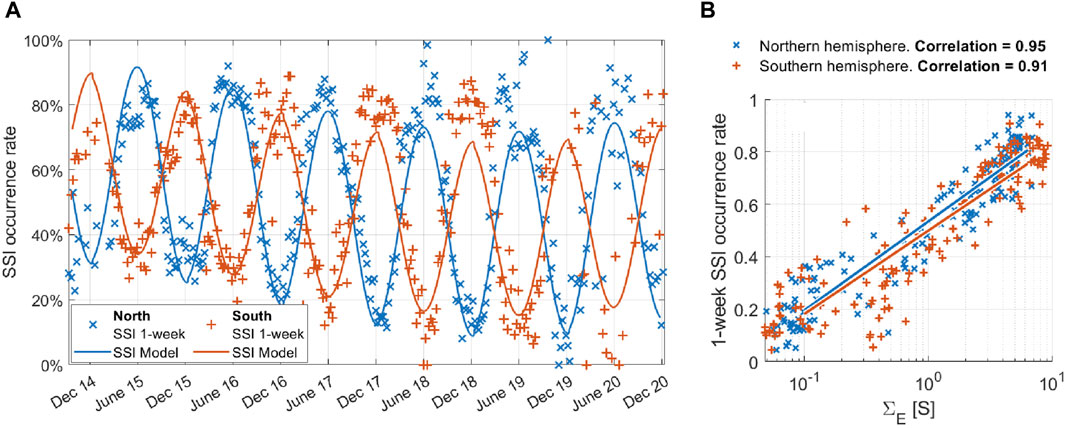
Figure 1. Data reproduced from Figure 2 in Ivarsen et al. (2021b) demonstrating how the local season is the main driver of steepening in F-region polar cap density spectra. Occurrences of steepening density spectra inside the ionospheric polar caps. The blue and orange colors refer to the northern and southern hemispheres, respectively. In both panels, each cross datapoint represents occurrence rate within a one-week period. In panel (A), these occurrence rates are plotted against time for the 6-year period of 2014–2020. A linear fit of the occurrence rate versus solar zenith angle (SZA) is plotted with a solid line and evaluated as a function of time, as the mean SZA within the polar caps varies predictably according to local season, meaning that a linear fit becomes a regular periodic function. Panel (B) shows the same data plotted against ${\mathrm{\Sigma }}_E$, the modeled Pedersen conductance within the E region, with the Pearson correlation coefficients indicated (see Ivarsen et al. (2021b) for details).

Figure 2

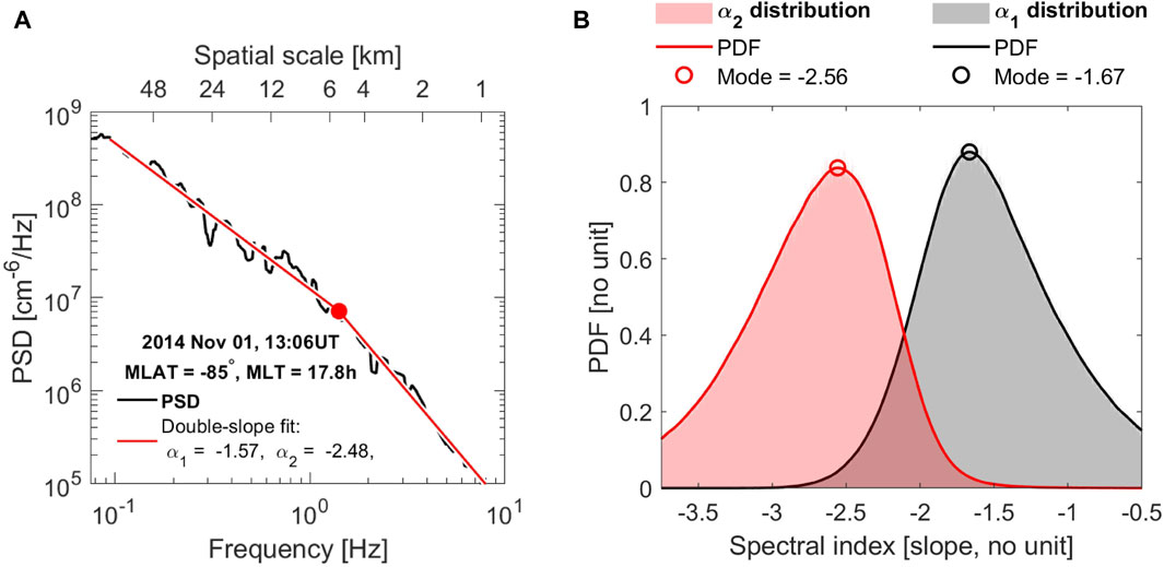
Figure 2. (A) Example density spectrum as measured by Swarm A on 1 November 2014 in the evening sector polar cap. The power spectral density (PSD) is shown on the $y$ axis, with frequency on the bottom $x$ axis. The latter is used to show irregularity spatial scale on the upper $x$ axis, using $L=v_{Sw}/f$, where $L$ is the spatial scale, $v_{sw}$ is the satellite velocity, and $f$ is the frequency. A double-slope fit is shown in solid red line, with the two slopes ${\alpha }_1$ and ${\alpha }_2$ indicated. (B) Distributions of ${\alpha }_1$ (black) and ${\alpha }_2$ (red) for all 2.7 million steepening density spectra observed by Swarm A in the high-latitude (poleward of $\pm 55°$ MLAT) F region (2014–2020). The probability density function is calculated as pdf $=c/(Nw)$, where $c$ is the number of elements in each bin, $N$ is the total number of elements, and $w$ is the width of the bin. With this definition, the integral over pdf yields the dimensionless number 1. The peak probabilities (modes) are indicated for both distributions.

Recently, Ivarsen et al. (2023b) compared the F-region steepening density spectra with kilometer-scale spectral density information from the E region. Using both space–ground conjunctions and statistical methods, the authors showed that the same kilometer-scale turbulent shapes were consistently observed both in the bottom and top ionosphere. Importantly, Ivarsen et al. (2023b) demonstrated that although solar zenith angle (SZA) (and thus solar EUV photoionization) is the driver of polar cap steepening spectra, the auroral electrojet (and thus the nightside aurora and substorm cycle) drives the steepening of spectra in the auroral region.

Accordingly, a central goal of the present study is to test the idea of a link between energetic precipitation and appearance of steepening F-region spectral slopes using in situ particle detector data. We use precipitating particle observations from the Defense Meteorological Satellite Program (DMSP) in conjunction with data from the European Space Agency’s Swarm mission. If precipitation-induced enhancements in the Pedersen conductance are the main cause of efficient irregularity dissipations in the absence of sunlight, we should find identical locations for the energetic electron or ion precipitations as well as F-region irregularity dissipation.

Given our interest in the dissipating density spectra, we need to address the role of non-dissipative density spectra and whether the total irregularity power is markedly decreased in the dissipative spectra. Surprisingly, we found no evidence that any excess irregularity power was removed from the F region by the high-energy diffuse aurora, leading us to conclude that energetic precipitation tends to cause a net gain in the observed F-region plasma irregularity power. Since F-region irregularities have very long field-aligned wavelengths (Ivarsen et al., 2021b, Appendix B), the observed auroral irregularities could plausibly originate in the E region, where the densities can drastically increase (Liang et al., 2021). Unstable gradients form at the edges of such pockets of ionization (Makarevich, 2017). With this interpretation, high-energy particle precipitation will both create and destroy F-region irregularities.

2 Methodology

As noted, we aggregate and analyze in situ data from two separate sources. To quantify the energy input from the magnetosphere, we use a database of precipitating electron and ion data from the SSJ instruments on board the DMSP F16, F17, F18, and F19 satellites. These satellites are in heliosynchronous dawn–dusk polar orbits that cover most of the dayside high-latitude ionosphere in the northern hemisphere and most of the nightside in the southern hemisphere, meaning that a statistical aggregate that combines both hemispheres will sample almost all local times. Notable exceptions to these are a dayside wedge of roughly $70°$ equatorward magnetic latitude (MLAT) between 11 h and 13 h magnetic local time (MLT) as well as a smaller nightside wedge of $65°$ equatorward between the same local times. In other words, the $65°$ midnight equatorward and $70°$ noon equatorward are inaccessible to scrutiny even after combining both hemispheres. The altitude of the satellites is around 840 km, meaning that they sample the topside of the F region. Of interest here are the data collected with the SSJ instrument, which comprises particle detectors that measure the energy fluxes of the precipitating electrons and ions through 19 energy channels from 30 eV to 30 keV at a sampling frequency of 1 s (Redmon et al., 2017). The satellites rotate in orbit to align the detector upwards along Earth’s field lines. To supplement the precipitating particle observations, we show data from the SSIES (electron density) and SSUSI (far-ultraviolet, or FUV, auroral imaging) instruments.

Next, we use a database of high-resolution plasma density observations from the EFI instrument on the Swarm A satellite (Friis-Christensen et al., 2008). Swarm A’s orbit covers all magnetic local times in a 131-day cycle at an altitude of around 460 km. The 16 Hz advanced plasma density calculations are produced by the currents through the Swarm faceplate in conjunction with the on-board Langmuir probe Knudsen et al. (2017).

As indicated, we subject both datasets to a statistical aggregate. The time periods for the two datasets used in the present study overlap but are not equal. Specifically, the DMSP database extends from 2014 through 2016 (3 years), while the Swarm A data from 6 years of operation from the end of 2014 until 2020 are used nominally; however, for direct statistical comparisons between the DMSP and Swarm A, we use the same time period (2014–2016). This three-year period follows the 24th solar cycle peak, with anticipated strong signals from the solar wind and magnetospheric drivers. All data considered in the present study are ordered by MLT and MLAT, where we use the altitude-adjusted corrected geomagnetic coordinate system (Baker and Wing, 1989). Space-based conjunctions in this coordinate system thus take into account the curvature of the Earth’s field lines. Lastly, Swarm A slowly sweeps through local times in a 131-day cycle, while DMSP that consists of four satellites in slightly varying dawn–dusk orbits samples most local times on a regular basis. It is worth noting here that the DMSP was not designed to sample all local times systematically and that dawn and dusk are subsequently favored over noon and midnight.

We subjected the plasma density observations to a particular power spectral density (PSD) analysis introduced by Ivarsen et al. (2019) that has been extensively documented in Ivarsen et al. (2021b). To briefly summarize, the analysis entails automatic calculation and detection of the steepening plasma density spectra. For the density spectra themselves, we used a method based on Welch’s PSD (Welch, 1967; Tröbs and Heinzel, 2006). To identify the presence of spectral breakpoints, we first considered the PSD to conform to a dual-slope power law before fitting a piecewise linear Hermite function to the logarithm of the spectrum (D’Errico, 2017). If a spectral fit to the log of a spectrum shows a numerical difference between the first and second spectral slopes exceeding 0.8, with the second slope being steeper, we infer a spectral break associated with steepening.

In Figure 2A, we show a single example spectrum as a solid black line, with the double-slope linear fit shown in solid red. The slope or spectral index information is indicated, and the panel shows a spectrum that steepens after a breakpoint at around 5 km. As discussed in Ivarsen et al. (2021b), the spectral break must be found between the frequencies of 0.19 Hz and 6.5 Hz, corresponding to along-track spatial scales between 1.2 km and 39.9 km. Although comparatively narrow, this interval encompasses a key spatial scale in high-latitude ionospheric plasma physics: the transitional scale to a fully collisional regime at 2–3 km (Keskinen and Huba, 1990).

We perform the preceding analysis on 60-s segments of plasma densities sampled at high latitudes with a cadence of 5 s, meaning that the spectra overlap extensively. From this analysis, we extract and store the slopes for the steepening spectra along with a flag that indicates the presence of a steepening spectrum, separating moderately and severely steepening spectra. The criterion for the latter is that the second slope $({\alpha }_2)$ should be steeper than −2.6, for reasons that will be made clear shortly. In addition, we collect and store the density variances contained in 3-s segments after removing a 3-s second-order Savitzky–Golay filter. This quantity is equivalent to the total integrated irregularity power for scale sizes less than 23 km (3 s of orbital time) and reflects small-scale fluctuations in the plasma density. In Figure 2B, we show distributions for the two slopes ${\alpha }_1$ (black) and ${\alpha }_2$ (red) for all 2.7 million steepening spectra recorded in the high-latitude F region during the 2014–2020 period. Although the distributions are relatively wide, we observe that ${\alpha }_1$ has a peak probability at exactly −5/3, which Kolmogorov (1968) referred to as the so-called turbulent cascade, providing evidence that the density spectra in general steepen as a result of turbulence. The second spectral index, ${\alpha }_2$, tends to be considerably steeper when a breakpoint is inferred, with a peak probability at around −2.6. We are now in a position to justify our choice of −2.6 as the threshold index to delineate severely steepening spectra from those that steepen only moderately; −2.6 is the peak ${\alpha }_2$ value and also a value below which we find almost no ${\alpha }_1$ measurements. In other words, any spectrum that steepens with ${\alpha }_2<-2.6$ is steeper than the majority of steepening spectra and exhibits a value of ${\alpha }_2$ that exceeds the magnitude of any ${\alpha }_1$ measured.

Hereafter, the Severely Steepening Spectra Index (SSSI) refers to the occurrence rate of spectral steepening (with ${\alpha }_2<-2.6$) within a spatial or temporal bin. The Moderately Steepening Spectra Index (MSSI) then refers to the occurrence rate of having a steepening spectrum with ${\alpha }_2\ge -2.6$. As a working definition and for succinctness, we sometimes refer to these as dissipating and non-dissipating density spectra, respectively.

Lastly, to quantify the general presence of turbulent density power, we calculate the density variance within a 3-s running window, dubbed as the 3s root-mean-square (RMS) value. This quantity is sensitive to density irregularities smaller than 23 km.

3 Results

In Figure 3, we present a conjunction between Swarm A and DMSP F17 during moderate geomagnetic conditions $(K_p=3)$. Panel (a) shows the trajectories of the two satellites in geomagnetic coordinates, with the 5-min stretch of orbit constituting the conjunction indicated with a slightly thicker line. DMSP F17 orbited equatorward first, followed by Swarm A orbiting poleward 10 min later. The background colormap displays the FUV auroral emission intensity as measured by the SSUSI instrument on board the F17 satellite, and the solar terminator (on Earth’s surface) is indicated with a gray dashed line. Panels (b) and (c) show the color spectrograms of the electron and ion energy fluxes as measured by the SSJ particle detector instrument. Panel (d) shows the Swarm-measured plasma density at an altitude of 460 km in red and mapped to the DMSP orbit. The DMSP-measured plasma density at an altitude of 840 km is in turn shown by the black line, with values along the left $y$ axis. Panel (e) shows the 3-s density variance in black (left axis). The SSSI’s are seen in the red-shaded area, and their occurrence rate is given by the red trace; the MSSI’s are seen in the blue-shaded area and shown by the blue trace. The occurrence rates associated with both indices are shown on the right $y$ axis. The two bottom $x$ axes indicate the DMSP orbit trajectory to which the Swarm data are mapped.

Figure 3

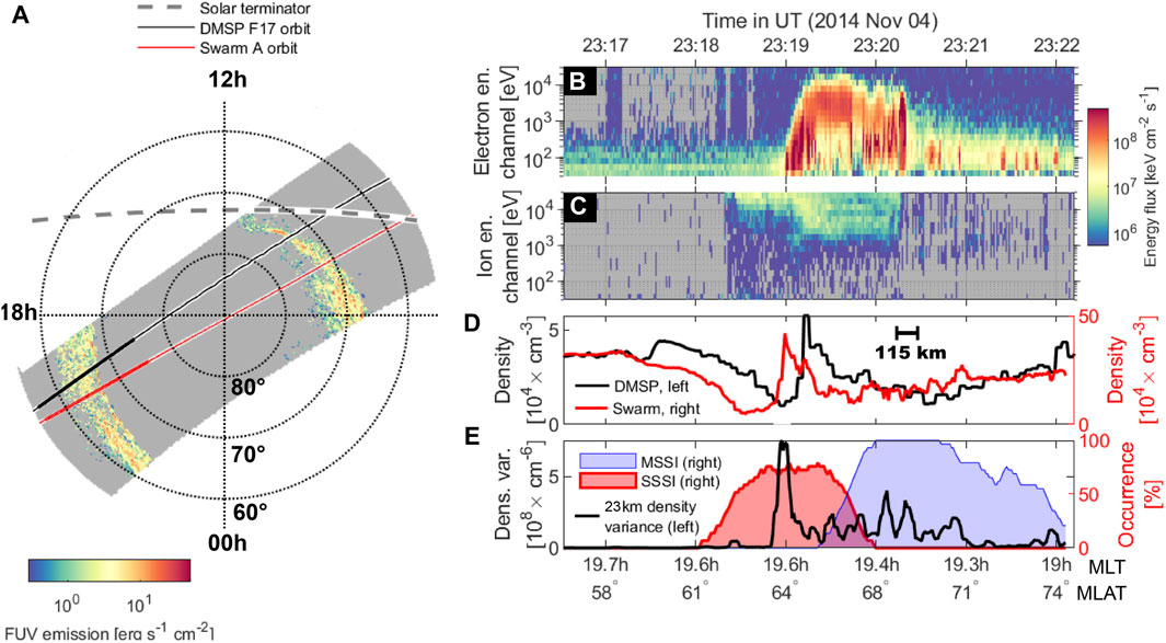
Figure 3. Parallel conjunction between Swarm A and DMSP F17 observations at 23:20 UT on 4 November 2014 in the northern hemisphere. (A) Orbital trajectories with FUV auroral emission intensity (from the SSUSI instrument) shown with a color scale. The stretches of the orbits identified as conjunctions are plotted with thicker lines. The solar terminator (on Earth’s surface) is shown by a dashed gray line. (B, C) DMSP SSJ precipitating electron and ion energy fluxes, respectively. (D) Swarm 16 Hz plasma density (red, right axis) mapped to the DMSP F17 orbit, with the DMSP-measured plasma density at 840 km in black (left axis). (E) Occurrence rates of moderately steepening spectra in a 30-s window (blue shaded area) and severely $({\alpha }_2<-2.6)$ steepening spectra (red shaded area). Ten-minute separation between the two orbits, with the DMSP leading and satellites orbiting in opposite directions. The Swarm data are mapped to the DMSP orbit.

The FUV auroral imaging confirms that although the orbits of the two satellites were separated by a few hundred kilometers, they were both sampling the same longitudinal auroral structure. The Swarm data appears 115 km equatorward of the DMSP data owing to spatial or temporal changes in the local conditions between the orbits. From the similarities between the two timeseries, we conclude that interactions between the aurora and plasma had not progressed substantially in the 10-min period separating the DMSP and Swarm orbits, which is consistent with the behaviors expected of quiescent arcs (Borovsky et al., 2019).

As evident from Figure 3B, the precipitation poleward of the longitudinally elongated auroral arc was characterized by soft (low-energy) electrons, while the equatorward portion saw intense, diffuse, and hard (high-energy) electrons as well as hard ion precipitation. Hard electron and ion precipitations generally provide optimal conditions for highly elevated Pedersen conductance in the E region (Vickrey et al., 1981; Fang et al., 2013). The 23 km (3 s) density variance (panel (e), left axis) contains several elevated spikes, showing that there are small-scale fluctuations in the plasma density, and the occurrence of steepening spectra remains high throughout the interval, with severely steepening spectra (SSSI, red shaded area) dominating the equatorward portion and moderately steepening spectra (MSSI, blue shaded area) dominating the poleward portion of the oval.

The SSSI shows a clear signal, and the density spectra steepen severely owing to an electrical connection with the enhanced E-region conductance induced by the aurora (Ivarsen et al., 2021b). It is noted that Swarm A’s observations are acquired in the F region at around 300 km above the E region, while the DMSP F17’s observations are obtained at even higher altitudes. We then observe a signal locally in the F region (steepening density spectra), but this signal is produced in the E region in response to particle precipitation originating in the magnetosphere. On the other hand, density spectra observed in the presence of soft, less-intense precipitations steepen only moderately. In the first case (elevated SSSI), we observe F-region irregularities that are strongly affected by processes far below and far above the satellite. In the second case (elevated MSSI), we observe F-region irregularities that are likely produced locally in response to soft-electron precipitation.

To shed further light on this issue, we show two additional conjunctions in Figure 4. The first occurred at 11:30 UT on 23 August 2016 between Swarm A and DMSP F18 in the southern hemisphere (upper five panels); the second occurred at 17:45 UT on 2 December 2014 when Swarm C and DMSP F17 were in the northern hemisphere (lower five panels). The layout of this figure is similar to that of Figure 3. In Figure 4, there is no significant delay between the satellites in either conjunction and were practically immediate. The satellites orbited in the same directions in the case of the upper five panels of Figure 4 and in opposite directions in the case of the lower five panels. In both cases, the DMSP satellites observed notable electron and ion precipitations with highly varying energies (panels (b, c, g, and h)). In both cases, the poleward edge of the auroral oval is associated with soft electrons and no ions, while the equatorward edge is associated with hard electrons and ions (the latter with one order of magnitude lower energy flux). At the same time, as shown in panels (e and j) of Figure 4, the Swarm-observed steepening spectra in the vicinities of precipitation structures exhibit characteristic behaviors; intense hard precipitations correspond to elevated SSSIs (red shaded areas in panels (e and j)), while the structures associated with softer precipitations are dominated by MSSIs (blue shaded areas).

Figure 4

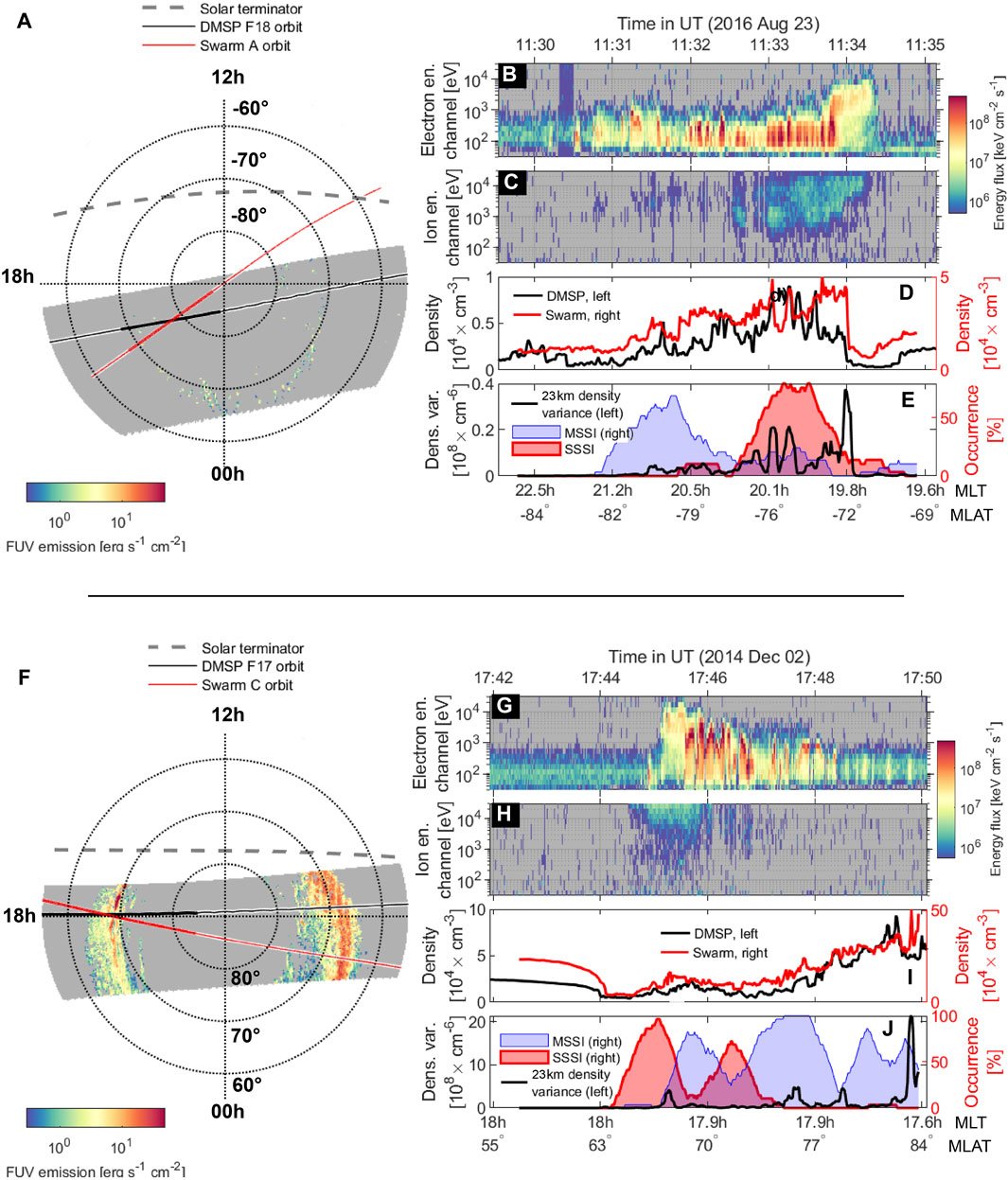
Figure 4. Two reasonably parallel conjunctions between Swarm A and DMSP F17. The top five panels show an event in the southern hemisphere at 11:30∼UT on 23 August 2016, while the lower five panels detail an event at 17:45∼UT on 2 December 2014 in the northern hemisphere. The 2016-conjunction occurred with a five-minute delay while the 2014-conjunction was immediate with no delay. Swarm data is mapped to the DMSP orbit. (A, F): orbital trajectories, with FUV auroral emission intensity (from the SSUSI instrument) shown with a colorscale. The stretches of orbits identified as conjunctions are plotted with a thicker line. The solar terminator (on Earth’s surface) is shown by a dashed gray line. (B, C, G, and H) show the DMSP SSJ precipitating electron and ion energy fluxes. (D, I) show Swarm 16∼Hz plasma density (red, right axis) mapped to the DMSP F17 orbit, with the DMSP-measured plasma density at 840∼km in black (left axis). (E, J) shows the occurrence rate of moderately steepening spectra in a 30 s window (blue shaded area) and the occurrence rate of severely (α₂<−2.6) steepening spectra (red shaded area). 10∼min separate the two orbits, with DMSP leading, and the satellites orbited in opposite directions. The Swarm data is mapped to the DMSP orbit.

Close conjunctions of the type shown in Figures 3, 4 are unfortunately not observed often as the temporal and spatial separations between the two satellites are usually too large for accurate determination of the associated boundaries. However, as we show in the next section, we can compare the two datasets over time using statistical scrutiny to compensate for the lack of immediate conjunctions.

In our statistical approach, we quantify geomagnetic activity using the SME index from the SuperMAG initiative (Gjerloev, 2012); it is an excellent indicator of the total nightside integrated auroral power (Newell and Gjerloev, 2011). Hereafter, we use the term “storm-time” to signify times of elevated SME indexes. This term does not refer to the onset of geomagnetic storms or magnetospheric substorms; instead, it is simply meant to indicate the instances of strongly elevated geomagnetic disturbances. In a statistical aggregate, we bin the DMSP and Swarm data from 2014, 2015, and 2016, where we combine data from the two hemispheres to ensure that all local times are sampled. There is precedence for such combination (see Newell et al., 2010), even as hemispherical asymmetries are not addressed. Motivated by the case studies presented above, we separate the hard from soft electron precipitations by integrating the incident energy fluxes through energy channels of 30–650 eV (soft energy flux) and 940–30,000 eV (hard energy flux). As the precipitating ions predominantly ionize the E region (Fang et al., 2013), we include the total integrated ion energy flux in the hard energy flux characterization.

The statistical relationships between the observed particle precipitations and steepening density spectra are presented in Figure 5 for the local winter climatologies. We define the local season as 131-day intervals centered on the respective solstices. Over this lengthy time period, the Swarm satellite samples every local time, while the DMSP satellites will have sampled all local times capable. Statistical data for the summer and equinox seasons are presented in Figure 7. In Figure 5, panels (a, b, e and f) show quantities binned by MLT and MLAT (geomagnetic noon being at the top of the plots and dawn to the right). The quantities of interest are the SSSI (a), hard energy flux (b), MSSI (e), and soft energy flux (f). Panels (c, d, g, and h) are data binned in terms of the SME index ($x$ axes, logarithmic) and MLAT ($y$ axes). In this representation, we combine data from the midnight sector (21 h$<$MLT$<$3 h), whose area is indicated with the solid black line in panels (a, b, e, and f). By limiting our scope to the midnight sector, we effectively remove the statistical MLT dependencies in the data, safely allowing us to partition (bin) the data by MLAT. Since the auroral oval expands in MLAT with increasing geomagnetic activity, this mode of representation has clear benefits; the equatorward expansion of the auroral oval results in a steady linear descent of the quantities to lower MLATs. Finally, in panels (c, d, e, and f), the regions within which the hard energy fluxes exceed $10^{11}$ keV ${\text{cm}}^{-2}{s}^{-1}{\text{ster}}^{-1}$ are bounded by the dashed black contours.

Remarkably, the ${\mathrm{\Phi }}_{\text{Hard}}>10^{11}$ keV ${\text{cm}}^{-2}{s}^{-1}{\text{ster}}^{-1}$ contour line captures the storm-time increase in the SSSI near-perfectly (Figure 5C). For MLATs equatorward of $\sim \pm 72°$, the SSSI and ${\mathrm{\Phi }}_{\text{Hard}}$ colormaps are virtually interchangeable despite originating from two completely different data sources.

Figure 5

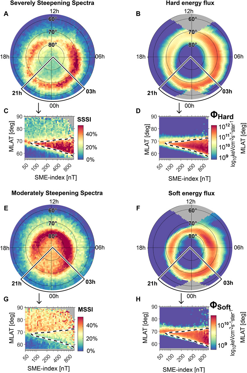
Figure 5. Four quantities central to the present work are binned first by (A, B, E, F) MLT-MLAT and then by (C, D, G, H) SME-MLAT for local winter conditions. The SME data are combined from the midnight sector (21 h$<$MLT$<$3 h, indicated with a black wedge) for both hemispheres. The quantities are (A, C) SSSI, (B, D) electron energy flux, (E, G) MSSI, and (F, H) soft energy flux. In panels (c, d, e, and f), the dashed black lines indicate contours of the constant hard energy fluxes equal to $10^{11}$ keV ${\text{s}}^{-1}{\text{cm}}^{-2}{\text{ster}}^{-1}$.

To illustrate the degree to which the distributions are matched, we show in Figure 6A linearly spaced contour lines of the constant SSSI occurrence rate during local winter in the midnight sector (red lines); overlaid, in blue color, we show the logarithmically spaced contour lines of the constant hard energy flux magnitude. Panel (b) shows the soft energy flux with the same logarithmic contour lines. We observe that the contour lines for the red and blue distributions are largely parallel to each other and are spaced in equal intervals; the two sets of contour lines are so similar that they can be applied interchangeably to describe both quantities. One represents an energy input to the ionosphere (hard electrons and ions), while the other represents an avenue for energy dissipation (severely steepening density spectra). At first glance, the striking similarities indicate that the inferences made by Ivarsen et al. (2021b) are indeed correct in that there are observable increases in the dissipations of the F-region density spectra in the auroral region when an E region is available to accelerate the diffusion of the F-region irregularities.

Figure 6

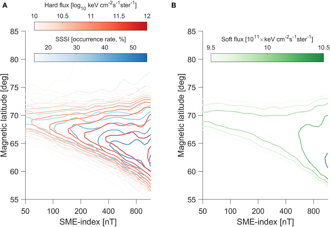
Figure 6. (A) Contours of the constant hard energy fluxes (logarithmically spaced, red color) and SSSI (linearly spaced, blue color), with (B) showing the corresponding observations for the soft energy fluxes. The figure combines data from panels (C, D, G) of Figure 5 (local winter, midnight sector, both hemispheres combined).

In Figure 7 we expand upon Figure 5, showing the SSSI, MSSI, 3s RMS, hard energy flux, and soft energy flux, all binned in terms of the SME index and MLAT (using local midnight data) for all three seasons. Each column corresponds to one of the five quantities, while each row corresponds to a local season (again combining data from the northern and southern hemispheres). The black dashed contours encloses bins in which the hard energy fluxes exceed $10^{11}$ keV ${\text{cm}}^{-2}{s}^{-1}{\text{ster}}^{-1}$ on average (in each season separately). First, we note that the energy fluxes (fourth and fifth columns) do not vary much with season, so any seasonal trends are likely to be caused by changes in the plasma dynamics and EUV photoionization rates. Second, we observe that the regions with elevated SSSIs in the auroral zone (first column) are largely similar across all seasons and that the ${\mathrm{\Phi }}_{\text{Hard}}>10^{11}$ keV ${\text{cm}}^{-2}{s}^{-1}{\text{ster}}^{-1}$ contour lines captures these increases excellently. However, looking at MLATs poleward of the auroral region, we see that the SZA (and hence solar EUV photoionization) is the main predictor of SSSI (see Figure 1), with a clear maximum during local summer.

Figure 7

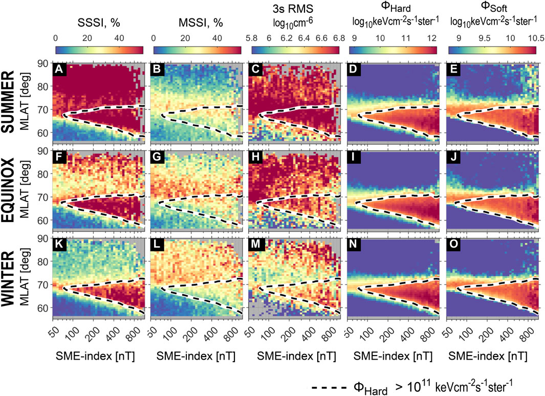
Figure 7. Five quantities (one for each column) binned by MLAT and SME, with each row representing the local season (one for each row) for combined observations from both hemispheres. Each panel considers data from the midnight sector (21 h$<$MLT$<$3 h). In each panel, the black dashed line indicates the contour of the constant hard energy flux for that season.

Another inference that can be made from Figure 7 is that the F-region 3s RMS quantity (a measure of small-scale irregularity power) follows the hard energy flux rather faithfully at auroral latitudes (Figure 7M). The F-region observations could then largely reflect the E-region irregularities that are being created and destroyed by hard electron precipitations or their effects on the E-region plasma. Electrostatic irregularities on scales exceeding 1 km in size should have long field-aligned wavelengths (Ivarsen et al., 2021b, Appendix B), so that the spectral quantities at kilometer scales should be mapped between the E and F regions (Ivarsen et al., 2023b). Conversely, the 3s RMS quantity is likewise elevated inside the polar cap but without any particle precipitation. This leaves the convection electric field as the primary cause of irregularities inside the polar caps through F-region plasma instabilities (Makarevich, 2017). In the auroral region, it is possible that the precipitation structure itself is mapped from the E region or that the precipitation structure is used as the seed for the growth of instabilities of the order of a few to tens of kilometers in the E region. The results in the E region acting as a source of the F region turbulence (instead of a sink) when hard energy precipitations are present.

In contrast, the MSSI is weakest during local summer (Figure 7B), and there is no link between MSSI and auroral precipitation (panels (b, g, and l)). In the next few paragraphs, we elucidate these inferences.

Our thesis, in summary, is as follows: in the presence of precipitation ionizing the E region, severely steepening spectra act as markers for electrostatic plasma irregularities that tend to be electrically connected to a highly conducting E region. Conversely, moderately steepening spectra act as markers for plasma irregularities that tend to be disconnected from a highly conducting E region. This interpretation is consistent with all the figures shown so far. The case studies (Figures 3, 4) were based on data from darkness; the regions of elevated MSSIs were largely co-located with soft precipitating energy fluxes, whereas the regions of elevated SSSIs were largely co-located with hard energy fluxes. In Figure 7B, the polar caps are subject to a constant solar EUV photoionization, and irregularities disconnected from the E region (MSSIs) are largely absent, except for a modest band on the poleward side of the auroral oval; panel (a) shows that this region is associated with a very high occurrence rate for severely steepening spectra. On the other hand, during local winter (panel (l), third row), the polar caps receive very little sunlight, and the moderately steepening spectra here dominate the polar cap regions. Tantalizing as this interpretation may be, other important factors are surely contributing to the picture; these factors include plasma turbulence associated with polar cap patches as well as precipitation-induced effects of the trans-polar arcs and polar rain, which are outside the scope of the present report.

Lastly, the third column of Figure 7 shows that small-to-intermediate-scale ($<23$ km) F-region density fluctuations prevail at higher latitudes. As this quantity has units of ${\text{cm}}^{-6}$, it is sensitive to the absolute density, and its tendency to maximize during local summer may therefore not be surprising. We note that this could be an important factor given that the 3s RMS peak values during local summer apply to both hemispheres (as confirmed) despite the fact that high-latitude irregularities have been shown to exhibit opposite seasonal trends across the two hemispheres (Jin et al., 2019; Jin and Xiong, 2020). Still, the third column shows that the ${\mathrm{\Phi }}_{\text{Hard}}>10^{11}$ keV ${\text{cm}}^{-2}{s}^{-1}{\text{ster}}^{-1}$ contour lines outline regions of elevated density variances that stand out most clearly in winter but also seem to be present during all seasons.

Moreover, the density variance increases on the equatorward edge of the auroral region, where the midnight spectra steepen most drastically (panels (a, f, and k) of Figure 7). In other words, increased F-region irregularity dissipations due to a highly conducting E region do not result in net removal of the meso-scale irregularity power but are rather associated with an increase.

Based on all of the above considerations, we draw the following conclusion: particle precipitation in the nightside aurora is a source of local winter conductivity enhancements, which drives F-region irregularity dissipation. However, the E region is also a potential source of kilometer-size structuring imposed by the precipitation itself or a source of larger-than-kilometer-size plasma instabilities that lead to irregularities being seeded by a combination of density gradients and electric fields. In addition, meter-scale E-region density irregularities generate very small-scale turbulences, thereby enhancing energy dissipation through enhanced forms of Joule heating (St-Maurice and Goodwin, 2021). At the kilometer scale and greater, E-region structuring due to precipitation structuring itself to the kilometer-size turbulence and greater is directly observable at F-region altitudes (Ivarsen et al., 2023b).

4 Discussion

We see evidence, both from the case studies and statistical representations, for the E region as a crucial modulator of density spectra in the F region. The question of particle precipitation being sufficiently hard then becomes a matter of utmost importance for the temporal evolution of the F-region irregularities. Indeed, the effect seems to be significant (with near-perfect co-location between the dashed line and red-colored region in Figure 5C) enough that one could entertain the notion that certain observations are essentially E-region irregularities being observed in the F region through mapping along the magnetic field lines. That is, the spectral shapes of some structures are dictated entirely by their electrical connection to the E region. This is where most of the incident precipitating energy flux is expected to end up in general (Newell et al., 2009). To elaborate further, we applied empirical calculations based on the observed energy channel data to estimate the ionization rate altitude profiles to some of our cases studies.

In panels (a, b, and c) of Figure 8, we reproduced the observations from the two conjunctions shown in Figure 4. In both cases, we marked the locations of two timestamps, indicated with the uppercase letters A and B. For these two timestamps, we show the incident particle spectra in panels (d and e) for DMSP F18 as well as (j and k) for DMSP F17. Here, the energy fluxes are shown along the $y$ axes and energy channels are along the $x$ axes. Electron channels are shown with black circles, while the ion channels are shown with filled grey circles. These particle spectra are then used to estimate the ionization rate altitude profiles using parameterized equations reported by Fang et al. (2010) and Fang et al. (2013). First, we treat each channel as a monoenergetic beam of precipitation (Chen et al., 2023). Next, we apply the equations in Fang et al. (2010) to each electron channel and those in Fang et al. (2013) to each ion channel. For the molecular composition of the Earth’s atmosphere, neutral densities, and neutral scale height, we used the MSIS modeled neutral atmosphere (Picone et al., 2002) with historical values of the AP index and $F_{10.7}$ solar radio flux. The resulting altitude profiles are robust indicators of the ionospheric altitude columns along which the incident energy fluxes are deposited (Fang et al., 2010) and hence the region of highest ionization production rate. To put these profiles into perspective, we indicate the approximate region of peak Pedersen conductivity (Kwak and Richmond, 2007) by the yellow shaded area.

Figure 8

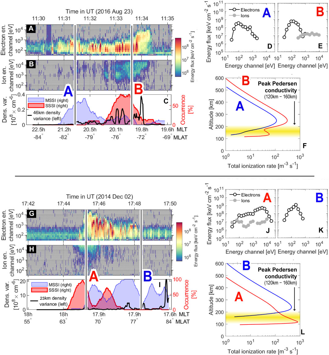
Figure 8. Ionization rate altitude profile calculations for the two case studies presented in Figure 4: (A–C, G–I) are reproduced from Figure 4, whose caption provides the detailed description. Two timestamps labeled with uppercase letters A and B and color coded refer to the particle spectra in (D, E, J, K). These spectra are used to produce the ionization rate profiles using equations from Fang et al. (2010); Fang et al. (2013) as well as the MSIS neutral atmosphere models. The resulting ionization rate profiles are shown in (F, L), where we also highlight the regions of peak Pedersen conductivity as reported by Kwak and Richmond (2007).

There are several interesting features in Figure 8. First, we clearly see that the soft electron precipitation typically found along the poleward edge of the auroral oval is largely unable to ionize the E region as it avoids the region of peak Pedersen conductivity to a great extent. This is consistent with our notion of moderately steepening density spectra as markers of plasma irregularities that are disconnected from the E region. In this case, F-region ionizations from softer precipitations can be intense, leading to density gradients that can in turn trigger instabilities. In contrast, the hard electron precipitations typically found along the equatorward edge of the auroral oval are more than capable of reaching the E region and can elevate the Pedersen conductance considerably. This is entirely consistent with our statistical picture, where the equatorward part of the oval has a conspicuous absence of moderately steepening spectra (Figure 7, panels (b, e, and h)).

Surprisingly, Figure 8F drives the point that ion precipitation can be an important source of E-region ionization. While it is known that the ion aurora only carries around 25% of the total energy flux (Newell et al., 2005), studies have found that the energy spectrum of the ion aurora typically peaks around $\sim 100$ keV (Gérard et al., 2001; Newell et al., 2005). In the DMSP SSJ data, no particles with energies greater than 30 keV were observed, but the observed ion precipitations predominantly carried energies higher than 1 keV, which we observed would always ionize the E region. This is exemplified from the 110-km bump in Figure 8F, where the moderate ion energy flux at timestamp B is capable of causing significant ionization in the region with maximized Pedersen conductivity.

4.1 High-energy particle precipitation and destruction of irregularities

We see a clear and unambiguous link between the severely steepening density spectra in the F region and high-energy particle precipitation capable of causing strongly enhanced E-region conductivity. This implies a real causal relationship that affects the F-region plasma irregularities with spatial scales larger than 1 km and that are able to map to or from a conducting E region. As initially argued by Ivarsen et al. (2021b), when the mapping is from the F region to a highly conducting E region, ambipolar electric fields associated with the irregularities are short-circuited by the E region (Vickrey and Kelley, 1982). Clearly, the enhanced conductivity is provided by the impact of high-energy precipitating particles in the polar night-time aurora. The dissipating F-region density spectra, which tend to display second slope values steeper than −2.6, indicate that the dissipations of small- and meso-scale ($<10$ km) plasma irregularities are accelerated by this connection to a conducting E region.

The above matches the behavior of severely steepening spectra observed inside the polar caps (Figure 1), but what about the moderately steepening density spectra? Thus far, we have suggested that they act as markers for spectra that are disconnected from the E region. We are now in a position to update Figure 1 with new knowledge, so we plot the long-term trends in the MSSI and SSSI occurrence rates: Figure 9 exhibits these results. Panels (a and c) show the scatterplots of SSSI versus average SZA poleward of the $\pm 82°$ MLAT (with a terminator in the E region at 110 km altitude) within the 27-day periods known as Carrington rotations (the solar rotation period with a characteristic periodicity in long-term geomagnetic activity). The blue (northern hemisphere) and orange (southern) circles show the SSSI, while the black and yellow hexagrams show the MSSI; the solid black lines are the linear trends for both (based on the empirical model described in Appendix B of Ivarsen et al. (2023a)). The MSSI grows in likelihood during the polar winter, while the SSSI grows in likelihood during the polar summer (also demonstrated by Figure 7). In Figure 9, panels (b and d) show all the Carrington rotations in sequence in a mode of representation akin to that in Figure 1. The spread in MSSI is different from the spread in SSSI (10%–90%): the MSSI only varies between 10% and 30% (though with a curious upward trend in the northern hemisphere towards solar minimum). Nevertheless, it is tempting to interpret the cyclical nature of the long-term MSSI as a signal produced by the relative prevalence of the plasma sampled, which is not electrically connected to the E region. However, does an elevated MSSI imply an increase in turbulence in general?

Figure 9

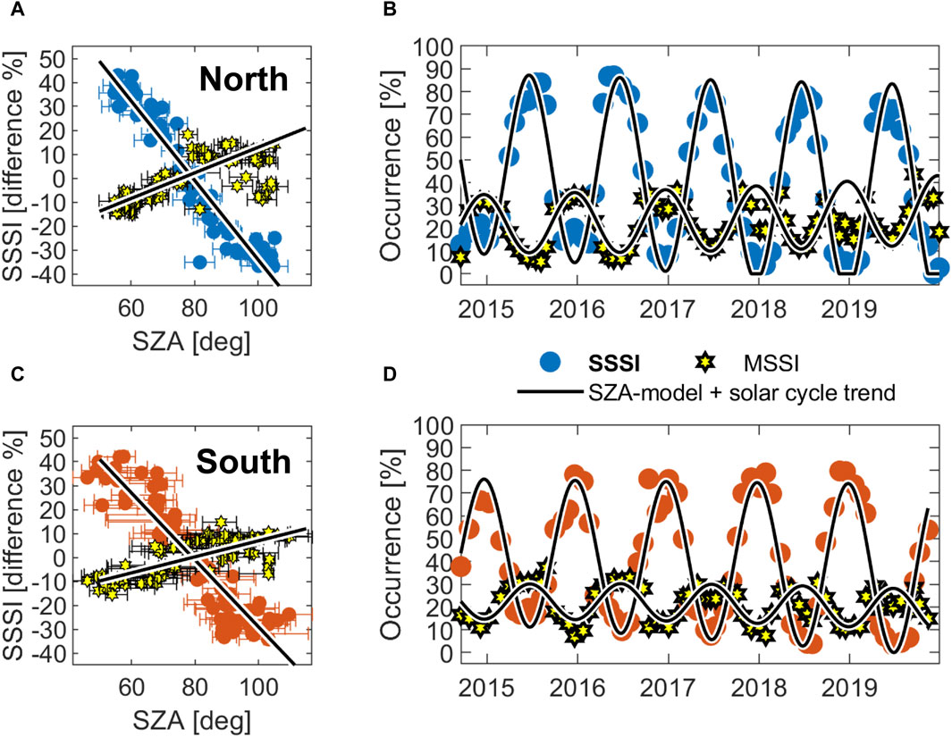
Figure 9. Data from Figure 1 with updated long-term trends in the polar cap occurrence rates of moderately steepening spectra (MSSI, black and yellow hexagrams). The blue (northern hemisphere) and orange (southern hemisphere) filled circles indicate the occurrence rates for SSSIs within each 27-day Carrington rotation period. The data were detrended and fitted according to the empirical model described in Appendix B of Ivarsen et al. (2023a). (A–C) show Carrington rotation bins in a scatterplot while panels B and D show those bins in chronological order.

It appears not. A comparison between panels (l and m) of Figure 7 (MSSI vs 3s RMS) reveals that the sharp drop-off in MSSI along the equatorward edge of the oval is co-located with an increase in mesoscale density variance. This increase is provided by energy injection by the high-energy electrons from the magnetosphere through the aurora or substorm cycle, as evidenced by the highly favorable co-locations in the first and fourth columns of Figure 7. We now examine these observations in the context of the energy input measured by the DMSP satellites. These comparisons (considering the auroral region) are performed on databases the cover the same length of observation time (2014–2016).

In our dataset, in the midnight sector, the hard energy flux constitutes 95% of the total energy flux, where “hard” here refers to electron energies between 1 and 30 keV (as well as the entire ion energy flux). Not all of this energy will end up in the E region, but the E region will receive exponentially more than the F region (Fang et al., 2010). In other words, the majority of the energy from the precipitating particles will be injected into the E region. In addition to the E region being the recipient of a considerable energy flux, the effective instability growth rates in the F region will be suppressed by highly efficient dissipation caused by the high-energy precipitation itself. The ratio of E-to-F-region conductance is thus likely to increase during storm-time (to see how this ratio affects F-region dissipation rates, see Figure 5 in Ivarsen et al. (2021a)). It is therefore not unreasonable to conjecture that the F-region irregularities observed in association with hard electron precipitations are in fact E-region structures that are mapped to F-region altitudes, a claim that finds support in recent observations (Ivarsen et al., 2023b).

5 Conclusion

Based on a large database of in situ observations of both ionospheric plasma and precipitating particles, we present a study of the complex interplay between precipitating particles and F-region ionospheric plasma. This interplay involves energy depositions and conductivity enhancements at the E-region and elevated ambipolar diffusion rates at the F-region altitudes. We used 3 years of precipitating electron and ion data from the DMSP F16, F17, F18, and F19 satellites as well as 3 years of high-resolution plasma density observations from the Swarm A satellite, in addition to three case studies containing some rare examples of good conjunctions.

The two databases in the present study are compared in Figures 5–7 and agree on a remarkably clear signal: in the equatorward side of the high-latitude regions, namely the auroral oval, high-energy electron precipitations cause observable widespread irregularity dissipations in the F region by enhancing E-region conductivity. Nevertheless, the total irregularity power remains high in regions dominated by dissipating density spectra. In other words, the irregularities that are dissipated were originally created by the hard precipitation. Local winter F-region irregularity dissipations caused by conductivity enhancements are interlinked with the occurrence of elevated irregularity power.

Our results clearly show that the in situ detection of steepening density spectra in the F region can be used to probe the complex interplay between particle precipitation and plasma irregularities in the high-latitude ionosphere. We tentatively suggest that severely $({\alpha }_2<-2.6)$ and moderately $({\alpha }_2\ge -2.6)$ steepening density spectra can act as markers for density irregularities that are respectively connected and disconnected to a highly conducting E region. Hence, more work is needed to assess the role of the moderately steepening spectra. However, the degree to which the SSSI traces the incident hard energy flux statistically is nothing short of excellent (Figure 6A). The fact that precipitating particles produce such distinct signatures visible in the plasma density spectra widens the avenue for utilization of in situ PSD analysis and supports continued application for the detection of steepening density spectra.

Data availability statement

The original contributions presented in this study are included in the article/Supplementary Material, and any further inquiries may be directed to the corresponding author.

Author contributions

MI: Conceptualization, Data curation, Formal analysis, Funding acquisition, Investigation, Methodology, Project administration, Resources, Validation, Visualization, Writing–original draft, Writing–review and editing. J-PS-M: Formal analysis, Funding acquisition, Supervision, Validation, Writing–review and editing. YJ: Conceptualization, Validation, Writing–review and editing. JP: Writing–review and editing, LB: Writing–review and editing. LC: Writing–review and editing.

Funding

The author(s) declare that financial support was received for the research, authorship, and/or publication of this article. This work is a part of the Lifetimes of Ionospheric Plasma Structures (LIPS) project at the University of Oslo and is supported in part by the Research Council of Norway (RCN) (grant no. 324859). The authors acknowledge the support of the Canadian Space Agency (CSA) (grant no. 20SUGOICEB); Canada Foundation for Innovation (CFI) John R. Evans Leaders Fund (grant no. 32117); Natural Science and Engineering Research Council (NSERC), International Space Mission Training Program supported by the Collaborative Research and Training Experience (CREATE) (grant no. 479771-2016); Discovery Grants Program (grant no. RGPIN-2019-19135); and Digital Research Alliance of Canada (grant no. RRG-FT2109).

Acknowledgments

The authors would like to thank D. J. Knudsen, J. K. Burchill, and S. C. Buchert for their work on the Swarm Thermal ion imager instrument.

Conflict of interest

The authors declare that the research was conducted in the absence of any commercial or financial relationships that could be construed as a potential conflict of interest.

Publisher’s note

All claims expressed in this article are solely those of the authors and do not necessarily represent those of their affiliated organizations or those of the publisher, editors, and reviewers. Any product that may be evaluated in this article or claim that may be made by its manufacturer is not guaranteed or endorsed by the publisher.

References

Baker, K. B., and Wing, S. (1989). A new magnetic coordinate system for conjugate studies at high latitudes. J. Geophys. Res. Space Phys. 94, 9139–9143. doi:10.1029/JA094iA07p09139

CrossRef Full Text | Google Scholar

Borovsky, J. E., Birn, J., Echim, M. M., Fujita, S., Lysak, R. L., Knudsen, D. J., et al. (2019). Quiescent discrete auroral arcs: a review of magnetospheric generator mechanisms. Space Sci. Rev. 216, 1. doi:10.1007/s11214-019-0619-5s11214-019-0619-5

CrossRef Full Text | Google Scholar

Braginskii, S. I. (1965). Transport processes in a plasma. Rev. Plasma Phys. 1, 205. doi:10.1007/978-1-4615-7799-7

CrossRef Full Text | Google Scholar

Chen, Z., Xie, T., Li, H., Ouyang, Z., and Deng, X. (2023). The global variation of low ionosphere under action of energetic electron precipitation. J. Geophys. Res. Space Phys. n/a, e2023JA031930. doi:10.1029/2023JA031930

CrossRef Full Text | Google Scholar

Cowley, S. W. H. (2000). Magnetosphere-ionosphere interactions: a tutorial review. Wash. D.C. Am. Geophys. Union Geophys. Monogr. Ser. 118, 91–106. doi:10.1029/GM118p0091

CrossRef Full Text | Google Scholar

D’Errico, J. (2017). Slm - shape language modeling - file exchange - MATLAB central. Natick, MA, Unites States: The MathWorks, Inc.

Google Scholar

Dungey, J. W. (1961). Interplanetary magnetic field and the auroral zones. Phys. Rev. Lett. 6, 47–48. doi:10.1103/physrevlett.6.471103/PhysRevLett.6.47

CrossRef Full Text | Google Scholar

Fang, X., Lummerzheim, D., and Jackman, C. H. (2013). Proton impact ionization and a fast calculation method. J. Geophys. Res. Space Phys. 118, 5369–5378. doi:10.1002/jgra.50484

CrossRef Full Text | Google Scholar

Fang, X., Randall, C. E., Lummerzheim, D., Wang, W., Lu, G., Solomon, S. C., et al. (2010). Parameterization of monoenergetic electron impact ionization. Geophys. Res. Lett. 37. Publisher: John Wiley and Sons, Ltd. doi:10.1029/2010GL045406

CrossRef Full Text | Google Scholar

Friis-Christensen, E., Lühr, H., Knudsen, D., and Haagmans, R. (2008). Swarm – an Earth observation mission investigating geospace. Adv. Space Res. 41, 210–216. doi:10.1016/j.asr.2006.10.008

CrossRef Full Text | Google Scholar

Gérard, J.-C., Hubert, B., Meurant, M., Shematovich, V. I., Bisikalo, D. V., Frey, H., et al. (2001). Observation of the proton aurora with IMAGE FUV imager and simultaneous ion flux in situ measurements. J. Geophys. Res. Space Phys. 106, 28939–28948. doi:10.1029/2001JA900119

CrossRef Full Text | Google Scholar

Gjerloev, J. W. (2012). The SuperMAG data processing technique. J. Geophys. Res. Space Phys. 117. doi:10.1029/2012JA017683

CrossRef Full Text | Google Scholar

Heppner, J. P., Liebrecht, M. C., Maynard, N. C., and Pfaff, R. F. (1993). High-latitude distributions of plasma waves and spatial irregularities from DE 2 alternating current electric field observations. J. Geophys. Res. Space Phys. 98, 1629–1652. doi:10.1029/92JA01836

CrossRef Full Text | Google Scholar

Huba, J. D., Hassam, A. B., Schwartz, I. B., and Keskinen, M. J. (1985). Ionospheric turbulence: interchange instabilities and chaotic fluid behavior. Geophys. Res. Lett. 12, 65–68. doi:10.1029/GL012i001p00065

CrossRef Full Text | Google Scholar

Ivarsen, M. F., Jin, Y., Spicher, A., and Clausen, L. B. N. (2019). Direct evidence for the dissipation of small-scale ionospheric plasma structures by a conductive E region. J. Geophys. Res. Space Phys. 124, 2935–2942. doi:10.1029/2019JA026500

CrossRef Full Text | Google Scholar

Ivarsen, M. F., Jin, Y., Spicher, A., Miloch, W., and Clausen, L. B. N. (2021a). The Lifetimes of plasma structures at high latitudes. J. Geophys. Res. Space Phys. 126, e2020JA028117. doi:10.1029/2020JA028117

CrossRef Full Text | Google Scholar

Ivarsen, M. F., Jin, Y., Spicher, A., St-Maurice, J.-P., Park, J., and Billett, D. (2023a). GNSS scintillations in the cusp, and the role of precipitating particle energy fluxes. J. Geophys. Res. Space Phys. 128, e2023JA031849. doi:10.1029/2023JA031849

CrossRef Full Text | Google Scholar

Ivarsen, M. F., St-Maurice, J.-P., Hussey, G., Spicher, A., Jin, Y., Lozinsky, A., et al. (2023b). Measuring small-scale plasma irregularities in the high-latitude E- and F-regions simultaneously. Sci. Rep. 13, 11579. Number: 1 Publisher: Nature Publishing Group. doi:10.1038/s41598-023-38777-4s41598-023-38777-4

PubMed Abstract | CrossRef Full Text | Google Scholar

Ivarsen, M. F., St-Maurice, J.-P., Jin, Y., Park, J., Miloch, W., Spicher, A., et al. (2021b). Steepening plasma density spectra in the ionosphere: the crucial role played by a strong E-region. J. Geophys. Res. Space Phys. 126, e2021JA029401. doi:10.1029/2021JA029401

CrossRef Full Text | Google Scholar

Jin, Y., Miloch, W. J., Moen, J. I., and Clausen, L. B. N. (2018). Solar cycle and seasonal variations of the GPS phase scintillation at high latitudes. J. Space Weather Space Clim. 8, A48. doi:10.1051/swsc/2018034

CrossRef Full Text | Google Scholar

Jin, Y., Spicher, A., Xiong, C., Clausen, L. B. N., Kervalishvili, G., Stolle, C., et al. (2019). Ionospheric plasma irregularities characterized by the Swarm satellites: statistics at high latitudes. J. Geophys. Res. Space Phys. 124, 1262–1282. doi:10.1029/2018JA026063

CrossRef Full Text | Google Scholar

Jin, Y., and Xiong, C. (2020). Interhemispheric asymmetry of large-scale electron density gradients in the polar cap ionosphere: UT and seasonal variations. J. Geophys. Res. Space Phys. 125, e2019JA027601. doi:10.1029/2019JA027601

PubMed Abstract | CrossRef Full Text | Google Scholar

Kelley, M. C. (1989). “Instabilities and structure in the high-latitude ionosphere,” in The Earth’s ionosphere. Editor M. C. Kelley (Academic Press), 345–423. doi:10.1016/B978-0-12-404013-7.50013-7

CrossRef Full Text | Google Scholar

Keskinen, M. J., and Huba, J. D. (1990). Nonlinear evolution of high-latitude ionospheric interchange instabilities with scale-size-dependent magnetospheric coupling. J. Geophys. Res. Space Phys. 95, 15157–15166. doi:10.1029/JA095iA09p15157

CrossRef Full Text | Google Scholar

Kivanc and Heelis, R. A. (1998). Spatial distribution of ionospheric plasma and field structures in the high-latitude F region. J. Geophys. Res. 103, 6955–6968. doi:10.1029/97JA03237

CrossRef Full Text | Google Scholar

Knudsen, D. J., Burchill, J. K., Buchert, S. C., Eriksson, A. I., Gill, R., Wahlund, J.-E., et al. (2017). Thermal ion imagers and Langmuir probes in the Swarm electric field instruments. J. Geophys. Res. Space Phys. 122, 2655–2673. doi:10.1002/2016JA022571

CrossRef Full Text | Google Scholar

Kolmogorov, A. N. (1968). The local structure of turbulence in incompressible viscous fluid for very large Reynolds numbers. Sov. Phys. Usp. 10 (6), 734. doi:10.1070/PU1968v010n06ABEH003710

CrossRef Full Text | Google Scholar

Kwak, Y. S., and Richmond, A. D. (2007). An analysis of the momentum forcing in the high-latitude lower thermosphere. J. Geophys. Res. Space Phys. 112. doi:10.1029/2006ja011910

CrossRef Full Text | Google Scholar

Liang, J., St-Maurice, J. P., and Donovan, E. (2021). A time-dependent two-dimensional model simulation of lower ionospheric variations under intense SAID. J. Geophys. Res. Space Phys. 126, e2021JA029756. doi:10.1029/2021JA029756

CrossRef Full Text | Google Scholar

Makarevich, R. A. (2017). Critical density gradients for small-scale plasma irregularity generation in the E and F regions. J. Geophys. Res. Space Phys. 122, 9588–9602. doi:10.1002/2017JA024393

CrossRef Full Text | Google Scholar

Newell, P. T., and Gjerloev, J. W. (2011). Evaluation of SuperMAG auroral electrojet indices as indicators of substorms and auroral power. J. Geophys. Res. Space Phys. 116. doi:10.1029/2011JA016779

CrossRef Full Text | Google Scholar

Newell, P. T., Sotirelis, T., and Wing, S. (2009). Diffuse, monoenergetic, and broadband aurora: the global precipitation budget. J. Geophys. Res. Space Phys. 114. doi:10.1029/2009JA014326

CrossRef Full Text | Google Scholar

Newell, P. T., Sotirelis, T., and Wing, S. (2010). Seasonal variations in diffuse, monoenergetic, and broadband aurora. J. Geophys. Res. Space Phys. 115. doi:10.1029/2009ja0148051029/2009JA014805

CrossRef Full Text | Google Scholar

Newell, P. T., Wing, S., Sotirelis, T., and Meng, C.-I. (2005). Ion aurora and its seasonal variations. J. Geophys. Res. Space Phys. 110. doi:10.1029/2004JA010743

CrossRef Full Text | Google Scholar

Oppenheim, M. (1997). Evidence and effects of a wave-driven nonlinear current in the equatorial electrojet. Ann. Geophys. 15, 899–907. Publisher: Copernicus GmbH. doi:10.1007/s00585-997-0899-z

CrossRef Full Text | Google Scholar

Phelps, A. D. R., and Sagalyn, R. C. (1976). Plasma density irregularities in the high-latitude top side ionosphere. J. Geophys. Res. 81, 515–523. doi:10.1029/ja081i004p00515JA081i004p00515

CrossRef Full Text | Google Scholar

Picone, J. M., Hedin, A. E., Drob, D. P., and Aikin, A. C. (2002). NRLMSISE-00 empirical model of the atmosphere: statistical comparisons and scientific issues. J. Geophys. Res. Space Phys. 107, 15–16. doi:10.1029/2002JA009430

CrossRef Full Text | Google Scholar

Prikryl, P., Jayachandran, P. T., Chadwick, R., and Kelly, T. D. (2015). Climatology of GPS phase scintillation at northern high latitudes for the period from 2008 to 2013. Ann. Geophys. 33, 531–545. doi:10.5194/angeo-33-531-2015

CrossRef Full Text | Google Scholar

Redmon, R. J., Denig, W. F., Kilcommons, L. M., and Knipp, D. J. (2017). New DMSP database of precipitating auroral electrons and ions. J. Geophys. Res. Space Phys. 122, 9056–9067. doi:10.1002/2016JA023339

PubMed Abstract | CrossRef Full Text | Google Scholar

Spicher, A., Miloch, W. J., and Moen, J. I. (2014). Direct evidence of double-slope power spectra in the high-latitude ionospheric plasma. Geophys. Res. Lett. 41, 1406–1412. doi:10.1002/2014GL059214

CrossRef Full Text | Google Scholar

St-Maurice, J.-P., and Goodwin, L. (2021). Revisiting the behavior of the E-region electron temperature during strong electric field events at high latitudes. J. Geophys. Res. Space Phys. 126, 2020JA028288. doi:10.1029/2020JA028288

CrossRef Full Text | Google Scholar

Tröbs, M., and Heinzel, G. (2006). Improved spectrum estimation from digitized time series on a logarithmic frequency axis. Measurement 39, 120–129. doi:10.1016/j.measurement.2005.10.010measurement.2005.10.010

CrossRef Full Text | Google Scholar

Tsunoda, R. T. (1988). High-latitude F region irregularities: a review and synthesis. Rev. Geophys. 26, 719–760. doi:10.1029/RG026i004p00719

CrossRef Full Text | Google Scholar

Vickrey, J. F., and Kelley, M. C. (1982). The effects of a conducting E layer on classical F region cross-field plasma diffusion. J. Geophys. Res. Space Phys. 87, 4461–4468. doi:10.1029/JA087iA06p04461

CrossRef Full Text | Google Scholar

Vickrey, J. F., Vondrak, R. R., and Matthews, S. J. (1981). The diurnal and latitudinal variation of auroral zone ionospheric conductivity. J. Geophys. Res. Space Phys. 86, 65–75. doi:10.1029/JA086iA01p00065

CrossRef Full Text | Google Scholar

Welch, P. (1967). The use of fast Fourier transform for the estimation of power spectra: a method based on time averaging over short, modified periodograms. IEEE Trans. Audio Electroacoustics 15, 70–73. doi:10.1109/tau.1967.11619011109/TAU.1967.1161901

CrossRef Full Text | Google Scholar