Acceleration of an interplanetary shock through the magnetosheath: a global hybrid simulation

According to most observations and simulations, interplanetary shocks slow down when they propagate through the magnetosheath. In this article, we present results from a self-consistent global hybrid PIC simulation of an interplanetary shock which, by contrast, accelerates as it propagates through the magnetosheath. In this simulation, the solar wind upstream of the interplanetary shock is set up with an Alfvén Mach number M_A = 4.5 and the interplanetary magnetic field (IMF) is set up to be almost parallel to the y direction in GSE coordinate system. The ‘planet’ is modelled as a magnetic dipole with no tilt: the dipole is in the GSE’s z direction. In the ecliptic plane (Oxy), which contains the interplanetary magnetic field (IMF), the magnetic field lines are piling up against the magnetopause, and the velocity of the interplanetary shock decreases from 779 ± 48 km/s in the solar wind down to 607 ± 48 km/s in the magnetosheath. By contrast, in the noon-meridian plane (Oxz), which is perpendicular to the IMF, the velocity of the interplanetary shock in the magnetosheath can reach values up to 904 ± 48 km/s. This study suggests that interplanetary shocks can accelerate as they propagate through the magnetosheath. This finding, reported here for the first time, could have important implications for space weather, as it corresponds to the case where an interplanetary shock catches up with a low Alfvén Mach number solar transient such as an interplanetary coronal mass ejection.

1 Introduction

Interplanetary Coronal Mass Ejections (ICMEs) are well-known to be efficient drivers of geomagnetic activity (Burlaga, 1988; Gonzalez et al., 1999). Their high probability of including a large and long-lasting southward magnetic field component provides favourable conditions for triggering geomagnetic storms (Li et al., 2018). Their propagation at high speed in the interplanetary medium often generates a shock and a turbulent sheath which precede them and can also be geoeffective (Huttunen and Koskinen, 2004; Yermolaev et al., 2012; Katus et al., 2015). More generally, interplanetary (IP) shocks, associated or not with solar transients, are also considered to be efficient drivers of geomagnetic activity (Tsurutani and Gonzalez, 1997; Gonzalez et al., 1999; Lugaz et al., 2016). Despite the progress made in understanding the interaction of interplanetary shocks with the geomagnetic environment, there is still much to be learned. In recent years, there has been a growing recognition that when considering the coupling of the solar wind with the magnetosphere, it is essential to take into account the interfacing role played by the magnetosheath (e.g., Vörös et al., 2023). Therefore, an important question to consider is how interplanetary shocks propagate through the magnetosheath and are modified throughout this propagation.

Observations by several space missions of a single interplanetary shock at different points throughout its propagation during a magnetosheath crossing can only occur occasionally (Koval et al., 2005; Koval et al., 2006b; Koval et al., 2006a). Previous magnetohydrodynamic (MHD) simulations of the interaction of interplanetary shocks with the terrestrial bow shock have brought some important insights and also showed the complexity of this process (Koval et al., 2005; Samsonov et al., 2006; Samsonov et al., 2007; Šafránková et al., 2007; Němeček et al., 2010; Pallocchia et al., 2010; Goncharov et al., 2015). They have demonstrated that the impact of the interplanetary shock causes first an earthward motion of the bow shock which then moves outward later on (Samsonov et al., 2006; Samsonov et al., 2007; Šafránková et al., 2007). The interaction contributes to trigger instabilities propagating through the magnetosheath as predicted by Grib et al. (1979); Grib (1982). This is supported by observations confirming the presence of a fast-forward shock (Šafránková et al., 2007) in the magnetosheath after the interaction between an interplanetary shock and the bow shock. While the general solution to the Riemann problem predicts up to seven discontinuities, the fastest discontinuity propagating through the magnetosheath (a forward shock) is often still referred to as the interplanetary shock. We adopt this convention throughout the present article.

The magnetohydrodynamic (MHD) simulations cited above have consistently demonstrated that interplanetary shocks slow down when propagating through the magnetosheath. Most observational studies also support this finding (e.g., Villante et al. (2004); Koval et al. (2005); Koval et al. (2006b)). A telling case study by Zhang et al. (2012) using THEMIS observed an interplanetary shock, initially propagating at about 380 km/s in the solar wind, which interacted with the bow shock and transmitted a fast shock wave propagating at about 300 km/s and a second discontinuity propagating at about 140 km/s through the magnetosheath. They also found that this interaction could even affect the inner magnetosphere and plasmasphere, which demonstrates its important role in magnetospheric physics.

To go beyond these first global MHD descriptions of the interaction between an IP shock and the terrestrial bow shock requires taking into account kinetic effects since the ion dynamics is a fundamental component of shocks’ dynamics. In recent years, global hybrid particle-in-cell simulations—where the ions are treated as macroparticles and the electrons as a fluid—have successfully been used to model the geomagnetic environment subjected to various interplanetary conditions. The development of an ion foreshock upstream of Earth’s bow shock when the interplanetary magnetic field is in quasi-parallel conditions is a well-known example of the impacts of the ion dynamics on the geomagnetic environment (Blanco-Cano et al., 2006; Karimabadi et al., 2014; Turc et al., 2015; Omelchenko et al., 2021). Kinetic effects are also crucial in quasi-perpendicular conditions: for example, the shock self-reformation (Hellinger, 2003; Lembège et al., 2009) is a kinetic effect that could trigger instabilities (Lowe and Burgess, 2003; Cazzola et al., 2023). Such global hybrid simulations of a realistic geomagnetic environment demand a fairly large simulation box broadly centred around the magnetic obstacle. Omidi et al. (2004) established that a magnetic dipole interacting with the solar wind should be strong enough to create a magnetopause with a stand-off distance D_p of at least 20 d_i (d_i is the ion skin depth) in order to form a magnetosphere that resembles Earth’s magnetosphere. Depending on the orientation of the interplanetary magnetic field, the main region of interest, and the main physical effects expected to play a role, the stand-off distance D_p of the magnetopause in global 3D hybrid particle-in-cell simulations has ranged widely from 25 d_i (Turc et al., 2015; Cazzola et al., 2023) to 120 d_i (Omelchenko et al., 2021). Importantly, only a few global hybrid particle-in-cell simulations have been conducted with time-varying interplanetary conditions. Some studies introduced a rotational discontinuity (Karimabadi et al. (2014), reporting on 2D simulations with D_p up to 300 d_i) or a magnetic cloud (Turc et al., 2015), but, to date, none included an interplanetary (IP) shock.

Another difficulty is the introduction of a propagating IP shock in a simulation box which already includes a standing planetary bow shock. Typically, in MHD simulations, jump conditions of an IP shock are introduced either by reproducing observational data or by applying the Rankine-Hugoniot equations (e.g., Spreiter and Stahara (1992; Spreiter and Stahara (1994); Koval et al. (2005); Koval et al. (2006b); Samsonov et al. (2006); Samsonov et al. (2007); Šafránková et al. (2007); Němeček et al. (2010); Pallocchia et al. (2010); Goncharov et al. (2015)). However, interplanetary shocks are highly dissipative structures that self-consistently create in their wake interplanetary sheaths which then develop during their propagation. Self-consistent numerical simulations of an interplanetary shock need very “long” simulation boxes that provide enough space for the shock to form, propagate and create a sheath in its wake. This IP shock’s sheath should also be of significant size compared to the magnetosheath itself in order for its interaction with the geomagnetic environment to be considered in isolation from the end of the interplanetary sheath and the following driver of the shock (such as an ICME’s core) if there is one.

In short, global simulations including both a self-consistent standing shock (the bow shock) and a self-consistent propagating shock (the interplanetary shock) together with its following sheath and driver are challenging. As a first step in this direction, and before considering a complete solar event, the present paper aims to focus on the self-consistent propagation of an interplanetary shock through the terrestrial magnetosheath. It describes a new method (Section 2), using the 3D hybrid particle-in-cell code LatHyS (Modolo, 2004), to self-consistently model both the geomagnetic environment (bow shock, magnetosheath, magnetopause) and the self-consistent formation of an interplanetary shock followed by a sheath as the solar wind is overtaken by a fast magnetic cloud. In Section 3 we analyse the propagation velocity of the IP shock in the magnetosheath and discuss the results in Section 4.

2 Methods

Figure 1 is a concept diagram of our simulation setup in the 3D hybrid PIC code LatHyS (Modolo, 2004). On the right-hand side of the box, we placed an obstacle consisting of a magnetic dipole and an absorbing sphere [in the same way as Turc et al. (2015)]. We injected a plasma representing the solar wind coming in from the left-hand side of the simulation box. The obstacle’s interaction with the solar wind self-consistently generates a bow shock, a magnetosheath and a magnetopause (see Section 2.1). From the left-hand side of the box, we then evolved the parameters of the injected plasma over time, using an analytical expression inspired by Burlaga (1988) to represent a fast magnetic cloud. In this simulation, the magnetic cloud takes the role of being a realistic driver for the interplanetary shock. Indeed, as it propagates through the solar wind, it overtakes the bulk plasma to self-consistently generate an interplanetary shock and sheath (see Section 2.2).

FIGURE 1

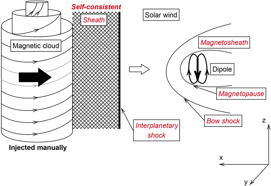
FIGURE 1. Simulation setup. A magnetic cloud is injected into the simulation box. It interacts with the solar wind to self-consistently create a shock and sheath. These structures interact with the geomagnetic environment, which itself self-consistently results from the interaction between the solar wind and a magnetic dipole. Structures that were injected (described by analytical expressions in the code) are noted in black. Structures that develop self-consistently are noted in red.

2.1 The geomagnetic environment

We used a setup similar to—albeit significantly larger than—(Turc et al., 2015). The box dimensions are 1500 cells in the x direction, 720 cells in the y direction and 660 cells in the z direction. Each grid cell is a cube of dimension ${(1d_i)}^3$, where d_i ≃ 93 km is the ion skin depth computed from the initial solar wind values. Therefore, we will talk interchangeably about x, y and z in terms of cell numbers or in terms of d_i.

The solar wind is injected from the left side of the simulation box (x > 0) as a superalfvénic plasma of protons neutralised by a massless electron fluid. The electron density is always equal to the ion density, and the electron temperature evolves to satisfy $n_e{T}_e^{5/3}=Constant$, starting with $T_e^{\text{sw}}=\mathrm{160,000}\text{\hspace{0.17em}K}$ at the injection side of the box. The injected solar wind has a density $n_i^{\text{sw}}=6({\text{ions/cm}}^3)$ with a bulk speed of V^sw = 400 km/s. It carries a magnetic field of amplitude B^sw = 10 nT which makes an 85° angle with the Sun-Earth axis: ${\mathit{B}}^{\text{sw}}=\left[B_x=B^{\text{sw}}\cos (85°),B_y=B^{\text{sw}}\sin (85°),B_z=0\right]$. The ions have a Maxwellian distribution of velocities corresponding to a temperature $T_i^{\text{sw}}=\mathrm{160,000}\text{\hspace{0.17em}K}$ which in turn corresponds to β = 0.5 in the solar wind. These values of density, velocity, temperature and β are typical of the observed solar wind (Venzmer and Bothmer, 2018), whereas the magnetic field amplitude—while still being realistic—is roughly twice the average value of the magnetic field carried by the observed solar wind. These choices make for a realistic scenario in the special case of a fairly high Alfvén speed (V_A = 89 km/s) and, a low Alfvén Mach number for the solar wind $(M_{\text{A}}^{\text{sw}}=4.5)$. More on this in the last paragraph of this subsection.

The “planet” (Earth) is represented in the code by a magnetic dipole placed at the origin (x = 0, y = 0, z = 0). The magnetic moment is aligned with the z-axis of the GSE—it has no tilt. The magnetic moment was chosen as M_simu ≃ 2 ⋅ 10²² Gauss.cm³ (or $900(\text{nT})\times {(14d_i)}^3$ in natural simulation units). The real magnetic moment of Earth is M_Earth ≃ 8 ⋅ 10²⁵ Gauss.cm³ (Bartels, 1936; Olson and Amit, 2006). Therefore, the radius of the simulated magnetopause is a factor ${\left(M_{\text{Earth}}/M_{\text{simu}}\right)}^{1/3}\simeq 16$ times smaller than the radius of the real magnetopause in similar interplanetary conditions. Balancing the magnetic pressure from this dipole with the dynamic pressure from the solar wind (Schield, 1969) leads to a magnetopause stand-off distance D_p = 34 d_i. This is safely above 20 d_i, which Omidi et al. (2004) showed to be a lower limit above which a simulated obstacle–or a real celestial body–interacting with the solar wind would display a magnetosphere similar to Earth’s. It is, however, not large enough to study smaller-scale phenomena such as those studied by Karimabadi et al. (2014) in 2D hybrid PIC simulations with D_p up to 300 d_i. Self-evidently, larger magnetosphere sizes require significantly increased computational resources, and the choice of the simulated magnetosphere size depends on the type of phenomena one wants to study. For example, in the case of a quasi-radial interplanetary magnetic field when the object of study is the interaction between the foreshock and the bow shock, known to lead to the occurrence of smaller-scale phenomena such as high-speed jets in the magnetosheath, it is reasonable to use D_p = 120 d_i (Omelchenko et al., 2021). In the case of high cone angles, where most of the bow shock is in a quasi-perpendicular situation, even though kinetic effects may still be important if the shock is supercritical (Hellinger, 2003; Lowe and Burgess, 2003; Lembège et al., 2009), an accurate description can still be obtained with D_p between 25 d_i and 40 d_i (Cazzola et al., 2023). In our simulation, the cone angle is 85°, which allows us to ignore the possibility of such small-scale events within the magnetosheath and to be reasonably confident that D_p = 34 d_i is enough for this simulation.

In our simulation, the interaction between the solar wind and the magnetic dipole leads to the self-consistent formation of a magnetosheath, delimited on each side by a bow shock and a magnetopause which reaches a stable equilibrium after $180{\mathrm{\Omega }}_{\text{ci}}^{-1}$. Note that throughout this text, ${\mathrm{\Omega }}_{\text{ci}}^{-1}\sim 0.96\text{second}$ serves as the time unit and refers to the inverse of the ion cyclotron frequency computed from the initial magnetic field amplitude in the solar wind: B^sw = 10 nT.

The behaviour of the plasma resulting from this setup is illustrated in Figure 2 which displays the amplitude of the plasma bulk velocity in three planes: the equatorial plane (Oxy), the noon-midnight meridian plane (Oxz), and a plane parallel to the terminator plane (Oyz) at x = −98d_i. The velocity of the plasma in the solar wind, taken as a reference value, is shown in grey; whereas regions where the plasma travels faster (or slower) than V^sw are shown in red (or blue). The magnetosphere, simply defined here as where the density is below 4 protons per cm³, is shown in white. The magnetic field lines are represented in panel (A) representing the ecliptic plane (Oxy). Initially, the magnetic field is almost aligned in the y direction in the solar wind, and the figure shows them piling up in the nose region of the magnetosheath and draping around the magnetopause. This results in a slowing down of the bulk plasma: the velocity is shown in dark blue in the nose of the magnetosheath (panel (A)). It then progressively accelerates along the flanks of the magnetopause (light blue) but generally remains slower in the magnetosheath than in the solar wind. There is an exception, visible in red in panels (B) and (C): along the northward and southward regions of the magnetopause, the bulk magnetosheath plasma travels faster than the solar wind.

FIGURE 2

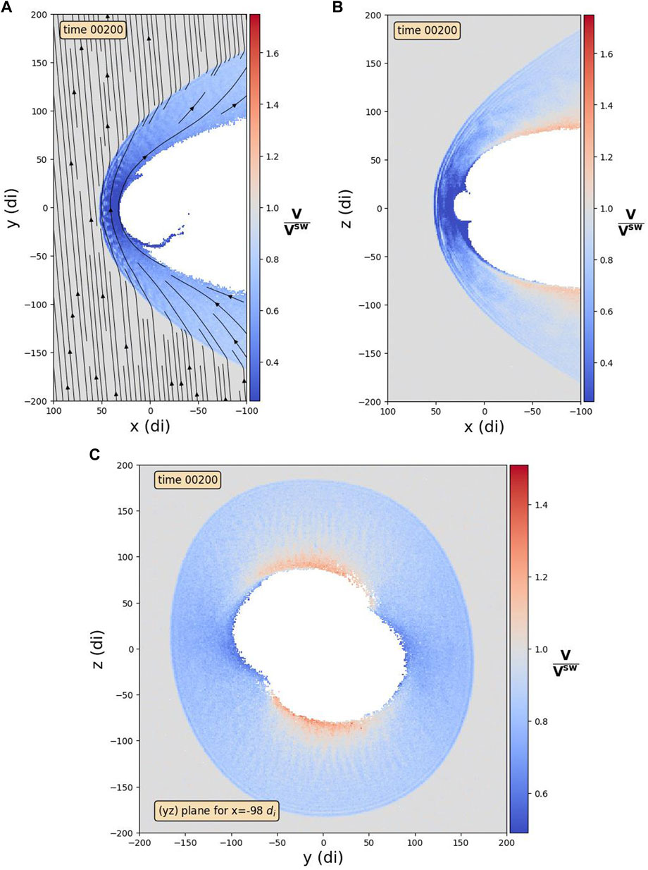
FIGURE 2. Colormap of the velocity in the magnetosheath in different planes. The velocity is represented as a ratio between the local velocity and the velocity in the solar wind (V^sw = 400 km/s). The regions where the velocity is equal to the velocity in the solar wind are shown in grey. Velocities slower or faster than V^sw are shown respectively in blue or red. The magnetosphere (simply defined here as where the density is below 4 particles per cm³) is shown in white. The panels represent the velocity of the plasma in, respectively; (A) the (Oxy) plane, (B) the (Oxz) plane, and (C) the plane (yz) for x = −98 d_i. The magnetic field lines are represented in the (Oxy) plane only (A), because the interplanetary magnetic field has no z component.

This setup–with a low Alfvén Mach number for the solar wind $(M_{\text{A}}^{\text{sw}}=4.5)$ and an interplanetary magnetic field (mostly in the y direction) being quasi-perpendicular to the solar wind flow–corresponds to conditions in which the plasma is expected to flow faster in some regions of the magnetosheath than it is in the solar wind. Such an effect was observed in similar conditions onboard ISEE, IMP 8 and Cluster, and explained by Chen et al. (1993), Lavraud et al. (2007), Lavraud et al. (2013) as emerging from a purely magnetic process, later called the “slingshot” effect. This effect operates for any orientation of the interplanetary magnetic field in the (yz) plane, perpendicular to the Sun-Earth axis. In our simulations, in the (Oxy) plane containing the magnetic field, the magnetic field lines pile up against the obstacle, thus increasing the magnetic pressure in the subsolar magnetosheath. In the subsolar region, their velocity slows down to almost zero while their open ends in the interplanetary medium still travel at the solar wind velocity: the magnetic field lines drape around the magnetopause and become highly curved, increasing the magnetic tension. In low Alfvén Mach number conditions with a large magnetic field, the magnetic forces dominate the plasma dynamics. The magnetic field lines can slip along the magnetopause’s flanks in the (Oxz) plane, perpendicular to the magnetic field. This causes the acceleration of the plasma by the Lorentz force with a roughly 50%/50% split between magnetic pressure force and magnetic tension (Lavraud et al., 2007). In addition, the plasma velocity enhancement contributes to an increase in the dynamic pressure on the north and south flanks of the magnetopause which becomes asymmetric as seen in Figure 2.

2.2 The magnetic cloud

There are several possibilities for introducing an interplanetary shock within a global numerical simulation, and the most commonly used is to introduce a step in several plasma parameters (velocity, density, magnetic field) compliant with the Rankine-Hugoniot equations. In our simulation, we decided to use a realistic driver: a magnetic cloud. While magnetic clouds are not the only drivers of interplanetary shocks, they do produce a sizeable fraction of them (Lindsay et al., 1994; Janvier et al., 2015). Using a driver also makes it possible to create a self-consistent interplanetary shock and the sheath following it. At the same time, it allows us to demonstrate a flexible approach to introducing solar transients in a global simulation.

Figure 3 summarises the temporal evolution of the plasma injected from the left-hand-side of the box. This temporal evolution creates a structure that is free to propagate and develop self-consistently. The magnetic cloud is injected from $t=60{\mathrm{\Omega }}_{\text{ci}}^{-1}$, which gives the geomagnetic environment enough time to be generated and reach a stationary state (at $t=180{\mathrm{\Omega }}_{\text{ci}}^{-1}$) before the magnetic cloud-driven interplanetary shock reaches the bow shock (at $t=216{\mathrm{\Omega }}_{\text{ci}}^{-1}$).

FIGURE 3

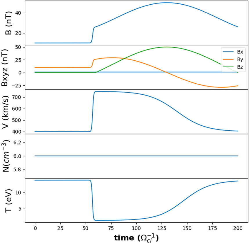
FIGURE 3. Temporal evolution of the characteristics of the injected plasma at the left side of the simulation box. From top to bottom: the magnitude of the magnetic field, its components, the bulk velocity, the ion density, and the ion temperature.

We followed the widely used model of Burlaga (1988), which describes a magnetic cloud as a force-free flux rope. We considered the magnetic cloud as a planar structure, which is reasonable because the typical size of a magnetic cloud at 1AU is 0.25AU (Lepping et al., 2006), which is much larger than the typical size of the geomagnetic environment $(\sim 10R_E\simeq 4\cdot 10^{-4}\text{\hspace{0.17em}AU})$. For simplicity, we also made the hypothesis that the magnetic cloud is travelling along the Sun-Earth line (Ox) and crossed at its centre; therefore the x-axis crosses the magnetic cloud radially and we can replace the radius of the magnetic cloud r in (Burlaga, 1988)’s model by x in our simulation. We kept B_x constant, which together with the planar hypothesis, ensures flux conservation (∇ ⋅B = 0). In order to avoid any effect related to a possible reconnection configuration which could affect the magnetopause and the magnetosheath, we chose to exclude any interplanetary magnetic field component oriented southward in the simulation. We decided to use a northward axial magnetic field so that the most interesting impacts of our event on the geomagnetic environment would come from the interplanetary shock and sheath rather than from the magnetic cloud. Indeed, choosing the axial component to be northward excludes the already well-studied magnetic reconnection effects that occur when a southward magnetic field interacts with the magnetopause (Dungey, 1961; Fairfield and Cahill, 1966; Tsurutani et al., 2020).

The time-dependent description of the magnetic field can be written as:

$\begin{array}{cc}\hfill B_z\left(t\ge t_0\right)=B_A\left(t\ge t_0\right)& =B_0{J}_0\left(a{u}_0\left(t-t_0\right)-2.4\right)\left(\text{Axial\hspace{0.17em}component}\right)\hfill \\ \hfill B_y\left(t\ge t_0\right)=B_T\left(t\ge t_0\right)& =B_0{J}_1\left(a{u}_0\left(t-t_0\right)-2.4\right)\left(\text{Tangential\hspace{0.17em}component}\right)\hfill \\ \hfill B_x\left(t\ge t_0\right)=B_R\left(t\ge t_0\right)& =Constant\left(\text{Radial\hspace{0.17em}component}\right)\hfill \end{array}(1)$

B₀ is the amplitude of the magnetic field at the magnetic axis of the flux rope, J₀ and J₁ are the two first Bessel functions, a determines the size of the magnetic cloud, u₀ is the bulk flow velocity, t₀ is the time at which we start injecting the magnetic cloud, and t is the time in the simulation. The 2.4 offset inside the Bessel functions is used to make t₀ the start of the magnetic cloud: indeed, J₀(2.4) = 0, which Burlaga (1988) defines as the edge of the magnetic cloud. Eq. 1 describe the magnetic field for times t ≥ t₀.

In order to avoid injecting discontinuities which would cause numerical issues, we used a hyperbolic tangent in order to obtain a smooth transition from the solar wind values (noted with the superscript “sw”) to the values at the leading edge of the magnetic cloud. In Eq. 2 which describes the magnetic field in the solar wind before the arrival of the magnetic cloud (for $t<t_0$), the parameter ${\tau }_0$

$\begin{array}{cc}\hfill B_z\left(t<t_0\right)& =B_z^{\text{sw}}+\left(0-B_z^{\text{sw}}\right)\frac{1}{2}\left(1+\tanh \left(\frac{t-t_0}{{\tau }_0}\right)\right)\hfill \\ \hfill B_y\left(t<t_0\right)& =B_y^{\text{sw}}+\left(B_0{J}_1\left(-2.4\right)-B_y^{\text{sw}}\right)\frac{1}{2}\left(1+\tanh \left(\frac{t-t_0}{{\tau }_0}\right)\right)\hfill \end{array}(2)$

To our knowledge, there is no available analytical model for the velocity and temperature of the plasma inside a magnetic cloud. In order to self-consistently create a shock and a sheath, the magnetic cloud needs to be faster than the solar wind by at least the Alfvén speed; i.e., V^mc − V^sw > V_A, where the superscript “mc” refers to the value in the magnetic cloud. We know from satellite observations that, statistically, the plasma inside a magnetic cloud is much colder than in the solar wind, and has a similar density (Regnault et al., 2020). Finally, we know that the magnetic cloud is a passing structure, so the plasma conditions should return to those of the solar wind after its passage. In order to take into account these observations, Eq. 3 describes the plasma’s bulk speed $V(t)$ and thermal speed $V^{\text{th}}(t)$ as follows:

$\begin{array}{ll}\hfill V\left(t\right)& =V^{\text{sw}}+\left(V^{\text{mc}}-V^{\text{sw}}\right)\times \left(\tanh \frac{t-t_0}{{\tau }_0}-\tanh \frac{t-t_1}{{\tau }_1}\right)\hfill \\ V_{\text{th}}\left(t\right)\hfill & =V_{\mathrm{th}}^{\text{sw}}+\left(V_{\mathrm{th}}^{\text{mc}}-V_{\mathrm{th}}^{\text{sw}}\right)\times \left(\tanh \frac{t-t_0}{{\tau }_0}-\tanh \frac{t-t_1}{{\tau }_1}\right)\hfill \end{array}(3)$

t₀ is the time at which the driver starts, and t₁ defines the time at which all the modified values start returning towards their quiet solar wind values. τ₀ and τ₁ control the sharpness of the transitions from quiet solar wind conditions to magnetic cloud conditions and back. We used the same t₀ and τ₀ as for the ramp of the magnetic field. V(t) and the temperature resulting from V_th(t) are represented in the third and fifth panels of Figure 3. As shown in the fourth panel of Figure 3, we kept the density of the injected plasma constant during the passage of the magnetic cloud.

At this stage, it is important to note that we have not introduced an interplanetary shock nor an interplanetary sheath in the simulation. Instead, we expect these structures to self-consistently emerge from the interaction between the magnetic cloud described in this section and the solar wind, which the magnetic cloud overtakes.

2.3 Summary of the simulation setup

Tables 1–3 summarise the simulation setup.

TABLE 1

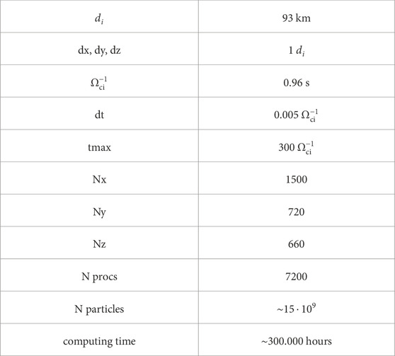
TABLE 1. Simulation parameters.

TABLE 2

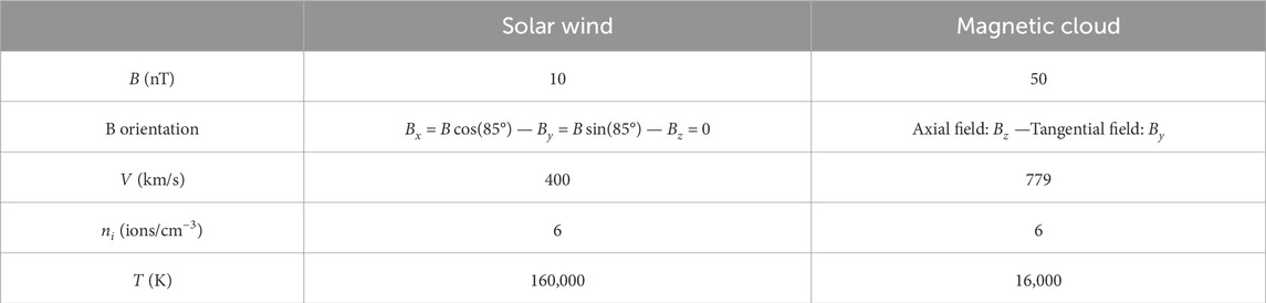
TABLE 2. Plasma parameters in the solar wind/magnetic cloud.

TABLE 3

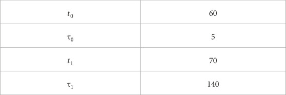
TABLE 3. Time parameters for the magnetic cloud, in ${\mathrm{\Omega }}_{\mathbf{ci}}^{-1}$

3 Results

3.1 The interplanetary shock and sheath

Figure 4 shows a snapshot (at $t=210{\mathrm{\Omega }}_{\text{ci}}^{-1}$) of the structure self-consistently produced by the propagation of the magnetic cloud as it overtakes the solar wind. The figure is plotted along the spatial x-axis. For clarity, the geomagnetic environment has been excluded from the plot (as we get closer to the magnetopause, the value of the planet’s magnetic field dwarfs those in the sheath/magnetic cloud and would make reading the figure difficult). From right to left, we can see: a stretch of solar wind, then the shock, self-consistently evolving and propagating, followed by the sheath, which has also self-consistently developed, and finally the start of the magnetic cloud.

FIGURE 4

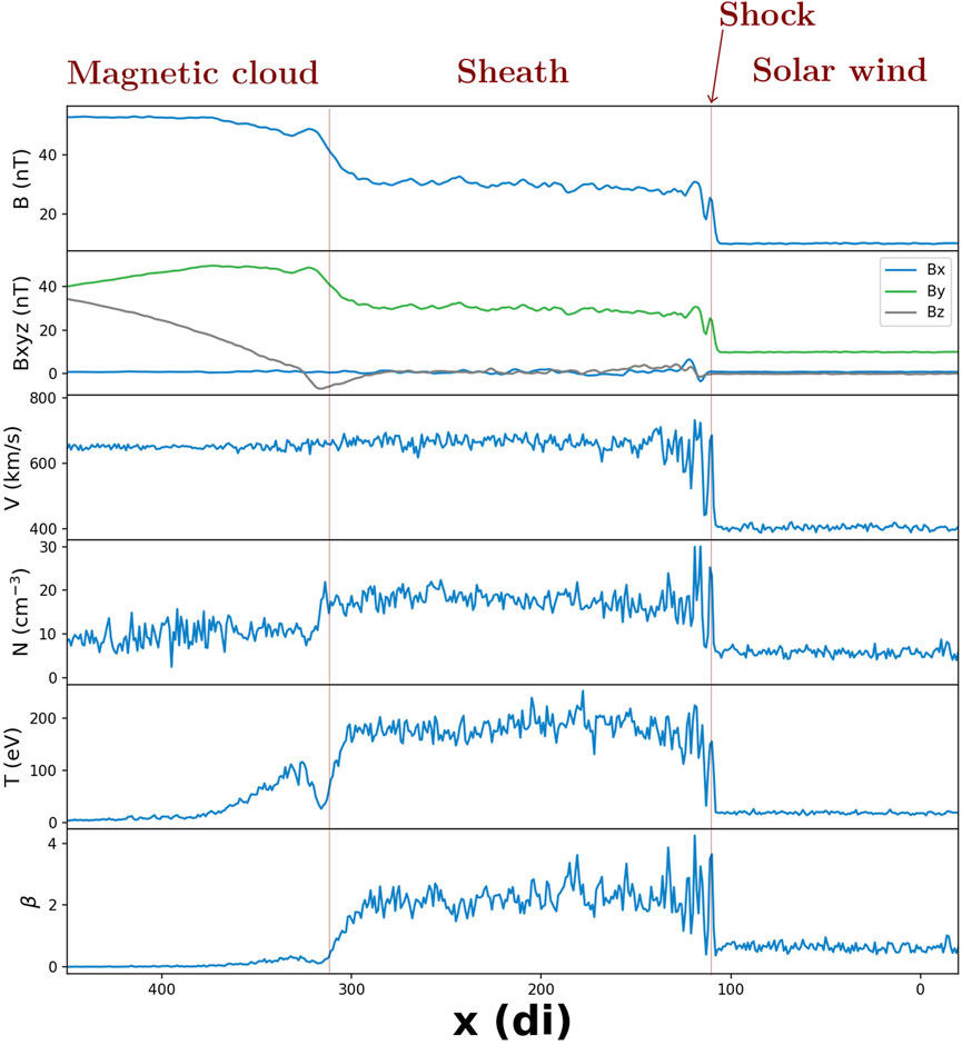
FIGURE 4. Main plasma parameters of the self-consistently created sheath at time = $210{\mathrm{\Omega }}_{\text{ci}}^{-1}$, shortly before its encounter with the geomagnetic environment. For clarity, Earth’s geomagnetic environment has been removed from this plot. Earth’s centre would be located at x =0.

The interplanetary shock in the solar wind has a velocity $V_{\text{shock}}^{\text{sw}}=779\text{\hspace{0.17em}km/s}$ in the GSE frame of reference, an Alfvén Mach number $M_{\text{Ashock}}^{\text{sw}}=\frac{V_{\text{shock}}^{\text{sw}}-V_{up}^{\text{sw}}}{V_{\mathit{Aup}}^{\text{sw}}}=4.2$; where $V_{up}^{\text{sw}}$ and $V_{\mathit{Aup}}^{\text{sw}}$ are, respectively, the velocity of the bulk plasma and the Alfvén speed upstream of the shock. The sheath thus obtained numerically captures the main characteristics of observed sheaths (e.g., Kilpua et al., 2017): the magnetic field amplitude $(\sim 30\text{\hspace{0.17em}nT})$, the plasma velocity $(\sim 650\text{\hspace{0.17em}km/s})$ and the density $(\sim 20\text{\hspace{0.17em}cc})$ are significantly higher than in the solar wind (B^sw = 10 nT, V^sw = 400 km/s, n^sw = 6 cc). The plasma beta $(\sim 2.5)$ and temperature $(\sim 2\cdot 10^6\text{\hspace{0.17em}K})$ are also elevated compared to the solar wind values (β^sw = 0.5 and T^sw = 1.6 ⋅ 10⁵ K), which is a consequence of significant heating at the shock. We can also see more fluctuations in the sheath than in the pristine solar wind, which is expected (e.g., Kilpua et al. (2017); Moissard et al. (2019); Pitňa et al. (2021)).

Table 4 summarises the main characteristics of the shock generated by the magnetic cloud overtaking the solar wind in this simulation.

TABLE 4

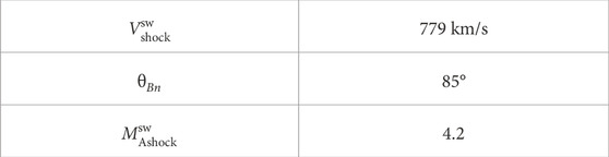
TABLE 4. Parameters of the resulting shock.

3.2 Velocity of the plasma

Figure 5, similarly to Figure 2, shows the plasma velocity represented as a ratio between the local velocity and the velocity in the pristine solar wind before the arrival of the shock, i.e., V^sw = 400 km/s. This is a snapshot of the plasma velocity when the shock has crossed the bow shock, travelled through the magnetosheath and reached the distance of approximately −60 d_i downtail. Further downtail, between −60 d_i and −100 d_i, the velocity distribution is exactly the same as in Figure 2 since the IP shock has not reached this region yet: the magnetosheath velocity is weaker than in the pristine solar wind except in the regions adjacent to the northern and southern boundaries of the magnetopause where it is larger. The magnetosheath downstream of the IP shock is now submitted to the impact of the turbulent sheath which has self-consistently developed in the wake of the IP shock. This induces some noteworthy differences. Some of these are expected: the overall size of the magnetosheath is reduced since the geomagnetic environment is now under greater pressure from the interplanetary medium, and the plasma velocity in the magnetosheath is larger due to the enhanced velocity in the interplanetary sheath relative to the pristine solar wind. Slightly less obvious differences can also be noted: the shape of the bow shock now presents a “trough” (also described in Pallocchia et al. (2010)), and finally, the magnetopause shows a slight indentation where it intersects the IP shock. The global patterns of the magnetic field and velocity do not change: magnetic field lines are still piling up in the nose of the magnetosheath, and the plasma velocity slows down in the nose region before re-accelerating toward the magnetopause’s flanks. Due to the still present “slingshot” effect, the velocity also reaches larger values near the northern and southern magnetopause than in the upstream interplanetary sheath.

FIGURE 5

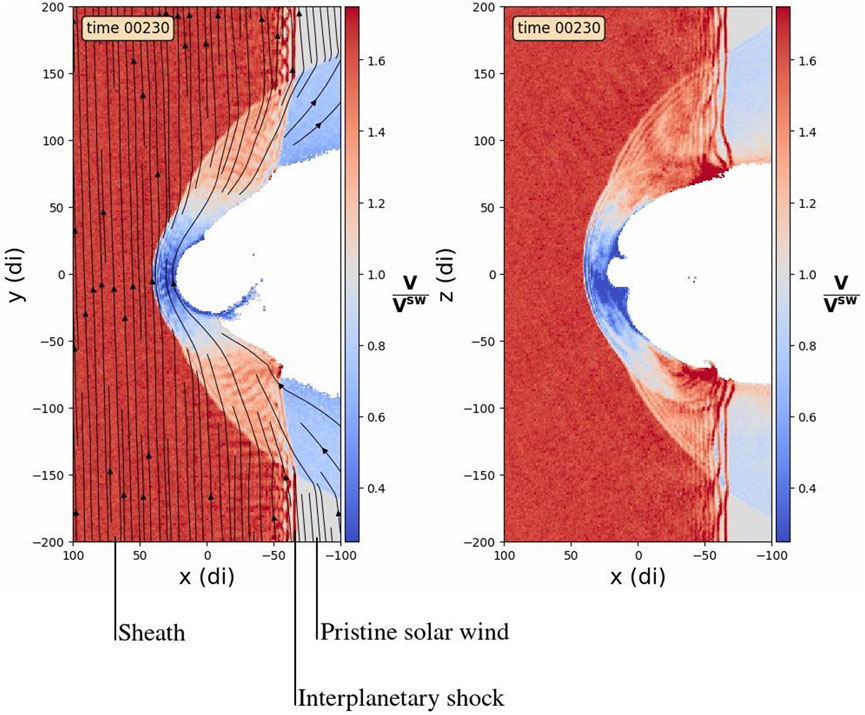
FIGURE 5. Colormap of the velocity in the magnetosheath in the equatorial (Oxy) and noon-midnight meridian (Oxz) planes. The velocity is represented as a ratio between the local velocity and the velocity in the solar wind prior to the arrival of the interplanetary sheath, V^sw = 400 km/s. The magnetic field lines are represented in the (Oxy) plane only, since the interplanetary magnetic field has no z component. The magnetosphere (density below 4 particles per cm³) is shown in white.

We now turn our attention to the interplanetary shock itself. Figure 5 shows the shape of the interplanetary shock as it is deformed during its propagation through the magnetosheath. The left-hand-side panel [panel (A)] shows that, similarly to previously published magnetohydrodynamic simulations, the interplanetary shock becomes concave in the magnetosheath (Koval et al., 2005; Samsonov et al., 2006; Šafránková et al., 2007; Pallocchia et al., 2010; Goncharov et al., 2015). This is interpreted as a slowing down of the IP shock as it travels through the magnetosheath: the parts of the IP shock closer to the magnetopause not only travel in a region where the plasma is much slower than anywhere else in the magnetosheath, they also encounter the bow shock earlier than the rest of the IP shock, and therefore have a longer time to propagate at a lower speed. The right-hand-side panel [panel (B)], however, tells a different story: in the plane perpendicular to the interplanetary magnetic field, the interplanetary shock becomes convex in the magnetosheath. This suggests that the interplanetary shock was locally accelerated as it travelled through the magnetosheath. Such a shock acceleration in the magnetosheath goes against previous observational and numerical studies on the topic, which all reported or predicted that interplanetary shocks always slow down as they travel through the magnetosheath (Villante et al., 2004; Koval et al., 2005; 2006b; a; Samsonov et al., 2006; Šafránková et al., 2007; Pallocchia et al., 2010; Goncharov et al., 2015).

3.3 Velocity of the interplanetary shock

Figure 6 shows the method used to estimate the velocity of the shock. We used a first detection of the position of the IP shock at a time T₁ and estimated its normal. Then we detected it again at a time $T_2=T_1+2{\mathrm{\Omega }}_{ci}^{-1}$. For each point of the shock detected at T₁, we measured the distance travelled between T₁ and T₂ along the normal of the shock. The white dots and arrows are here for illustration purposes only, as this process has been used at every y (or z) value along the shock.

FIGURE 6

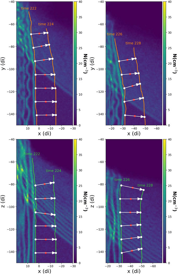
FIGURE 6. Color map of the plasma density on which two successive positions of the interplanetary shock are overlaid. The white dots are paired. To each dot on the left-hand-side shock corresponds an arrow which represents the normal of the shock. This arrow points to a corresponding dot on the right-hand-side shock.

Figure 7 shows the successive positions of the interplanetary shock at successive time steps: from its encounter with the bow shock (time 217), to a later position when it has propagated well beyond the terminator plane (time 232). On the left-hand-side panel [panel (A)], we depict the successive shock positions (orange lines) as seen in the ecliptic (Oxy) plane—where the magnetic field lines pile up and the plasma slows down. As it travels at a lower speed than in the solar wind, the delays accumulate and the shock can be seen to progressively become more concave. On the right panel [panel (B)], we are looking at the shock positions (green lines) in the noon-midnight meridian (Oxz) plane—where the magnetic “slingshot” effect takes place. As the shock travels locally faster than in the solar wind, the shock can be seen to progressively become more convex. In summary, when the initially planar IP shock in the pristine solar wind crosses the magnetosheath, it takes a distorted shape which seems to be related to the local plasma dynamics.

FIGURE 7

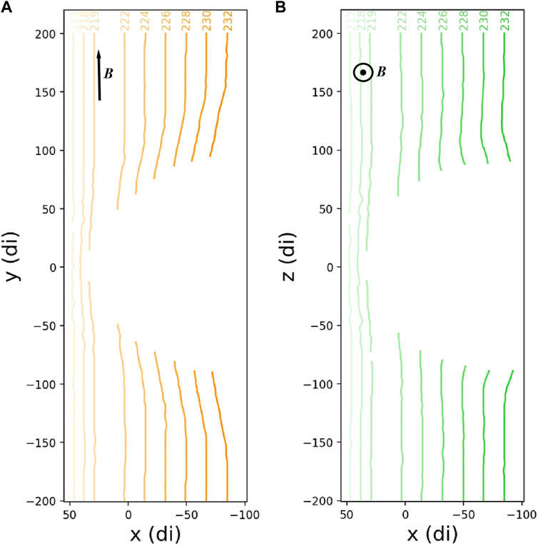
FIGURE 7. For both panels, the lines represent the successive position of the interplanetary shock as it propagates through the magnetosheath. The orange lines (left (A) represent the propagation in the ecliptic (Oxy) plane. The green lines (right (B) represent the propagation in the noon-midnight (Oxz) plane. For context, the interplanetary magnetic field is shown to mostly lie in the y direction.

We now aim to quantify the velocity change of the interplanetary shock as it travels through the magnetosheath. Figure 8 shows the absolute velocity of the shock at time steps 222, 224, 226, 228 and 230, which correspond to the times at which the concave/convex shapes are clearly observed in Figure 7. The velocity is represented against the distance from the planet’s centre along the y/z-axis. The colour code is the same as in Figure 7: orange in the equatorial plane (Oxy) in the upper panel (A) and green in the meridian plane (Oxz) in the bottom panel (B). The darker lines correspond to later times.

FIGURE 8

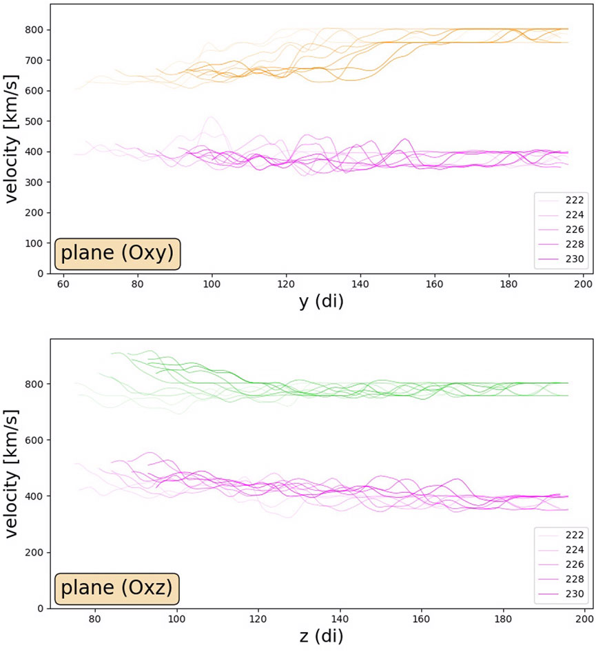
FIGURE 8. For both panels, the (orange/green) lines at the top represent the velocity of the interplanetary shock relative to the GSE frame. The figure has been “folded”: the x-axis represents the absolute distance from the centre of the obstacle. The purple lines at the bottom represent the velocity of the shock in the plasma frame. The lines are superposed from early in the propagation (pale) to late in the propagation (darker).

We can see that the values of the velocity fluctuate slightly. This is because the precision of the detection of the interplanetary shock is limited by the grid precision (dx = 1d_i). This leads to an uncertainty in the velocity: $\delta v=1d_i/2{\mathrm{\Omega }}_{ci}^{-1}=48\text{\hspace{0.17em}km/s}$. This uncertainty is clearly visible at large distances from the obstacle (y or z > 160d_i) where we are detecting the interplanetary shock in the solar wind: we previously estimated the velocity of the interplanetary shock in the solar wind at 779 km/s, however, this method of locally estimating the shock’s velocity returns somewhat fluctuating values around this estimate.

In the upper panel [panel (A)], the orange lines show that the velocity of the interplanetary shock decreases by roughly 170 km/s: from 779 ± 48 km/s in the solar wind down to 607 ± 48 km/s in the magnetosheath (minimum of the palest orange line corresponding to time 222). Then the IP shock gains back some speed: the minimum of the darkest orange line (which corresponds to time 230) is 695 ± 48 km/s. In the lower panel, the green lines show that the interplanetary shock in the (Oxz) plane slows down at first, from 779 ± 48 km/s in the solar wind to 730 ± 48 km/s in the magnetosheath (maximum of the palest green line corresponding to time 222). Then, the interplanetary shock accelerates up to 904 ± 48 km/s (maximum of the darkest green line corresponding to time 230) in the magnetosheath. The IP shock accelerates by around 125 km/s along the northern/southern flanks of the magnetopause, which are the regions in which the so-called “slingshot effect” is expected to play a role.

Whether it is decelerating or accelerating, the IP shock’s behaviour is very similar to that of the plasma just upstream of it. This seems to qualitatively correspond well to a hypothesis that was emitted by Koval et al. (2006b) that the velocity of the interplanetary shock is constant in the plasma frame (V_shock − V_up = Constant). In order to test this hypothesis, we have represented, still in Figure 8, the velocity of the IP shock in the plasma frame by the purple lines in both panels. In the upper panel [panel (A)], corresponding to the (Oxy) plane, the velocity goes from 375 ± 48 km/s in the solar wind to 410 ± 48 km/s. In the lower panel, corresponding to the (Oxz) plane, the velocity goes from 375 ± 48 km/s in the solar wind to 470 ± 48 km/s. In the (Oxy) plane, within the error bars, the lines are almost straight: there is no visible step at the bow shock and no curvature close to the magnetopause: the hypothesis that the IP shock’s velocity is constant in the plasma frame seems to be roughly verified. The validity of this hypothesis is less convincing in the (Oxz) plane.

4 Discussion

4.1 How previous arguments from the literature foreshadowed the present result

This article demonstrates that shocks could be accelerated in the magnetosheath, relative to the GSE frame of reference: indeed Figures 7, 8 show clearly that some parts of the interplanetary shock are accelerated in the magnetosheath. While the speed of the interplanetary shock was 779 ± 48 km/s in the solar wind, it went up to 904 ± 48 km/s in a small region of the magnetosheath. Two results from the pre-existing literature, taken together, hinted at such a possibility.

The first is the existence of well-established observations and simulations showing that the bulk plasma can accelerate in the magnetosheath (e.g., Chen et al. (1993); Lavraud et al. (2007; Lavraud et al. (2013)). As specified by (Lavraud et al., 2013), an interplanetary Alfvén Mach number below 5 is conducive to the formation of enhanced flows “on the […] flanks of the magnetosphere”. We set up our simulation with a solar wind’s Alfvén Mach number of 4.5 and an interplanetary magnetic field almost perpendicular to the Sun-Earth line and found that, indeed, these conditions led to the formation of a small region of accelerated plasma in the magnetosheath (see Figure 2).

The second is Koval et al. (2006b)’s hypothesis that an interplanetary shock may keep a constant speed in the plasma frame. This hypothesis, however, was based on a single case study, and—to our knowledge—does not have a theoretical explanation. We tested this hypothesis in Figure 8. Even when taking our relatively large uncertainties into account, it is clear that the velocity of the interplanetary shock in the plasma frame (purple lines in 8) is not quite always constant. Interestingly, though, Koval et al. (2006b)’s hypothesis seems to hold better for the decelerated part of the shock [upper panel (A)] than for the accelerated part of the shock [bottom panel (B)]—and the shock that they were observing was decelerating. Therefore, we propose to slightly amend Koval et al. (2006b)’s hypothesis and state, instead: As long as it is not accelerating, the interplanetary shock seems to keep an approximately constant speed in the plasma frame.

The strict validity of Koval et al. (2006b)’s hypothesis, together with Chen et al. (1993), Lavraud et al. (2007, Lavraud et al. (2013))’s “slingshot effect” would provide a straightforward argument for the possibility of accelerated shocks in the magnetosheath: if the velocity of interplanetary shocks is constant in the plasma frame, then an interplanetary shock propagating through a region of plasma accelerated by the slingshot effect would also accelerate. What we have shown in this article is that, while Koval et al. (2006b)’s hypothesis does not hold perfectly, the acceleration of interplanetary shocks still appears to be possible and in fact, to higher speeds than this hypothesis would predict.

4.2 Why this result was not reported before

The simulation of an accelerated shock reported in the present article may seem to go against previous studies on the subject—both observational and numerical—which all concluded that interplanetary shocks would decelerate in the magnetosheath (e.g., Villante et al. (2004); Koval et al. (2005); Samsonov et al. (2006; 2007); Šafránková et al. (2007); Němeček et al. (2010); Pallocchia et al. (2010); Goncharov et al. (2015)).

Lifting this paradox is straightforward: at 1AU, the median Alfvén Mach number of the solar wind is M_A = 8.4 (Veselovsky et al., 2010). All the authors of the magnetohydrodynamic simulations that we have cited (Koval et al., 2005; Samsonov et al., 2006; Samsonov et al., 2007; Šafránková et al., 2007; Němeček et al., 2010; Pallocchia et al., 2010; Goncharov et al., 2015) have—justifiably—set up their simulations with conditions typical of the observed solar wind: for example, Koval et al. (2006b) used M_A = 8.5, and both Samsonov et al. (2006) and Šafránková et al. (2007) used M_A = 8.2. Therefore, none of these previously reported numerical simulations were in conditions which could have led to the acceleration of the interplanetary shock in the magnetosheath.

In the interplanetary medium, M_A is below 5 less than 10% of the time (Veselovsky et al., 2010). Therefore, most observations of interplanetary shocks occur when the solar wind conditions are not conducive to the presence of accelerated flows in the magnetosheath (Lavraud et al., 2013). Furthermore, even when the interplanetary conditions are right, we have shown that the plasma, and therefore interplanetary shocks, should only be accelerated in a relatively small region of the magnetosheath: the region close to the magnetopause in which magnetic field lines can slip along the magnetopause and accelerate the plasma. Based on Figure 2, we can make a numerical estimate of the ratio between the volume of accelerated plasma and the volume of the rest of the magnetosheath: 3%. The probability for a satellite in the magnetosheath (at a random place and time) to observe an accelerated flow of plasma is, therefore, of the order of 10 % × 3 % = 0.3%. Likewise, we can expect that about 0.3% of all the shocks detected in the magnetosheath should be accelerated. This explains why previous observations by Villante et al. (2004); Koval et al. (2005, 2006a), reporting a total of 36 shocks detected in the magnetosheath, were only about $1-{\left((100-0.3)/100\right)}^{36}\simeq 10\%$ likely to report an encounter with an accelerated shock. Note, however, that in the simulation presented herein, the Alfvén Mach number is quite close to 5, and that lower Alfvén Mach numbers should lead to more extended acceleration regions, which could raise this relatively low likelihood of encountering an accelerated shock.

Interestingly, one of the shocks (31 January 1998) in Koval et al. (2006a) was in fact detected ahead of what a constant speed would predict, but the possibility of its acceleration was dismissed by the authors. Judging by the WIND measurements reported in Figure 3 of Koval et al. (2006a): n_i ≃ 8 cc, B ≃ 9 nT, V ≃ 360 km/s, we can estimate that the Alfvén Mach number of the solar wind upstream of this interplanetary shock was about M_A = 4.7. This is below M_A = 5, so according to the mechanism we proposed in the present article, this shock could indeed have been accelerated in the magnetosheath. While an intriguing prospect, it is difficult to decide whether the shock was actually accelerated, or (as suggested by Koval et al. (2006a)) not planar to the point of skewing the estimation of its speed. Indeed, other aspects do not go in the direction of the mechanism we proposed: (i) The interplanetary magnetic field’s non-radial component is in the y direction, which means that we would expect to see an accelerated shock for small values of y and close to the magnetopause in the (Oxz) plane. Interball-1 – which detected the shock in the magnetosheath at (−8, 25, 4)R_{E, GSE}–was not in the right place to see the accelerated portion of the shock. (ii) Accordingly, in the magnetosheath, the plasma upstream of the interplanetary shock did not travel faster than the solar wind.

4.3 Summary, future work and relevance for space weather

This paper presented results from a global hybrid PIC simulation which followed the interaction of two self-consistent structures: the geomagnetic environment, arising from the interaction between a magnetic obstacle and the solar wind; and an interplanetary shock propagating through a low Alfvén Mach number (M_A = 4.5) solar wind. We have shown herein that in such conditions, the velocity of the interplanetary shock reaches higher values in the magnetosheath (up to 904 ± 48 km/s) than it had in the solar wind (779 ± 48 km/s). While the plasma bulk flow is well known to be accelerated in such conditions, the possibility of the acceleration of an interplanetary shock had never been considered before—and indeed, all previous studies of the propagation of interplanetary shocks through the magnetosheath seemed to suggest that they would always decelerate. We have discussed that this was due to the relatively low probability of encountering one of these shocks (each individual encounter with an interplanetary shock in the magnetosheath has a less than 1% likelihood of corresponding to an accelerated section of the shock), and to a reasonable choice by authors of numerical simulations to favour typical solar wind conditions, in which we predict that, indeed, interplanetary shocks do always decelerate.

With the present paper showing the plausibility of the acceleration of an interplanetary shock through the magnetosheath at low upstream solar wind Alfvén Mach numbers, we can readily imagine that a targeted search for accelerated shocks—following a similar approach to Koval et al. (2005) and Koval et al. (2006a) but focusing on shocks propagating through an upstream plasma with a low Alfvén Mach number—may soon return observations of accelerated interplanetary shocks. Our task should be made easier by the fact that the number of spacecraft observing the magnetosheath has dramatically increased since 2006. An intriguing prospect is also the upcoming SMILE mission, which may be able to detect these shocks directly as they propagate through the magnetosheath, or indirectly, via the indentation they create at the magnetopause.

The most common circumstance in which the interplanetary plasma has a low Alfvén Mach number is during the occurrence of a magnetic cloud: magnetic clouds have a median Alfvén Mach number of 3.9 (Lavraud and Borovsky, 2008). Therefore, a typical scenario in which we would expect an interplanetary shock to be accelerated in the magnetosheath is when an interplanetary shock catches up with a magnetic cloud. Lugaz et al. (2016) showed that interplanetary shocks propagating into preceding CMEs were among the most likely shocks to lead to significant geomagnetic storms. Is it possible that the effect described in the present article plays a role in the geoeffectiveness of these interplanetary shocks? The increased velocity of the interplanetary shocks near the magnetopause could—for example,—enhance the Kelvin-Helmholtz instabilities on the flanks, further increasing the transfer of energy to the magnetosphere (see, e.g., Masson and Nykyri (2018)).

Data availability statement

The raw data supporting the conclusion of this article will be made available by the authors, without undue reservation.

Author contributions

CM: Conceptualization, Data curation, Formal Analysis, Funding acquisition, Investigation, Methodology, Software, Validation, Visualization, Writing–original draft, Writing–review and editing. PS: Conceptualization, Funding acquisition, Resources, Supervision, Writing–review and editing. DF: Conceptualization, Formal Analysis, Project administration, Supervision, Writing–review and editing. RM: Conceptualization, Software, Writing–review and editing.

Funding

The author(s) declare financial support was received for the research, authorship, and/or publication of this article. This work received financial support from the “Investissements d’avenir” program under the reference ANR-11-IDEX-0004-02 (Plas@Par). We are indebted to the ANR for the project TEMPETE (ANR-17-CE31-0016). We were granted access to the HPC resources of IDRIS under the allocation 2021-A0090410276 made by GENCI.

Acknowledgments

We thank Dr. Andrei Samsonov for useful discussions, and for confirming our results through running additional numerical simulations in similar solar wind conditions. Several students (Axel Bernal, Valentin Defayet, Virginia Cavicchi, Christopher Butcher, and Joel Richardson) at the University of York have started to search for accelerated shocks in observational data and provided much-appreciated discussions and enthusiasm for the research reported in this article.

Conflict of interest

The authors declare that the research was conducted in the absence of any commercial or financial relationships that could be construed as a potential conflict of interest.

Publisher’s note

All claims expressed in this article are solely those of the authors and do not necessarily represent those of their affiliated organizations, or those of the publisher, the editors and the reviewers. Any product that may be evaluated in this article, or claim that may be made by its manufacturer, is not guaranteed or endorsed by the publisher.

References

Bartels, J. (1936). The eccentric dipole approximating the Earth’s magnetic field. Terr. Magnetism Atmos. Electr. 41, 225–250. doi:10.1029/TE041i003p00225

CrossRef Full Text | Google Scholar

Blanco-Cano, X., Omidi, N., and Russell, C. T. (2006). Macrostructure of collisionless bow shocks: 2. ULF waves in the foreshock and magnetosheath. J. Geophys. Res. (Space Phys. 111, A10205. doi:10.1029/2005JA011421

CrossRef Full Text | Google Scholar

Burlaga, L. F. (1988). Magnetic clouds and force-free fields with constant alpha. J. Geophys. Res. 93, 7217–7224. doi:10.1029/JA093iA07p07217

CrossRef Full Text | Google Scholar

Cazzola, E., Fontaine, D., and Savoini, P. (2023). On the 3D global dynamics of terrestrial bow-shock rippling in a quasi-perpendicular interaction with steady solar wind. J. Atmos. Solar-Terrestrial Phys. 246, 106053. doi:10.1016/j.jastp.2023.106053

CrossRef Full Text | Google Scholar

Chen, S.-H., Kivelson, M. G., Gosling, J. T., Walker, R. J., and Lazarus, A. J. (1993). Anomalous aspects of magnetosheath flow and of the shape and oscillations of the magnetopause during an interval of strongly northward interplanetary magnetic field. J. Geophys. Res. Space Phys. 98, 5727–5742. doi:10.1029/92JA02263

CrossRef Full Text | Google Scholar

Dungey, J. W. (1961). Interplanetary magnetic field and the auroral zones. Phys. Rev. Lett. 6, 47–48. doi:10.1103/PhysRevLett.6.47

CrossRef Full Text | Google Scholar

Fairfield, D. H., and Cahill, L. J. (1966). Transition region magnetic field and polar magnetic disturbances. J. Geophys. Res. 71, 155–169. doi:10.1029/JZ071i001p00155

CrossRef Full Text | Google Scholar

Goncharov, O., Šafránková, J., and Němeček, Z. (2015). Interplanetary shock–bow shock interaction: comparison of a global MHD model and observation. Planet. Space Sci. 115, 4–11. doi:10.1016/j.pss.2014.12.001

CrossRef Full Text | Google Scholar

Gonzalez, W. D., Tsurutani, B. T., and Clúa de Gonzalez, A. L. (1999). Interplanetary origin of geomagnetic storms. Space Sci. Rev. 88, 529–562. doi:10.1023/A:1005160129098

CrossRef Full Text | Google Scholar

Grib, S., Brunelli, B., Dryer, M., and Shen, W.-W. (1979). Interaction of interplanetary shock waves with the bow shock-magnetopause system. J. Geophys. Res. Space Phys. 84, 5907–5921. doi:10.1029/JA084iA10p05907

CrossRef Full Text | Google Scholar

Grib, S. A. (1982). Interaction of non-perpendicular/parallel solar wind shock waves with the earth’s magnetosphere. Space Sci. Rev. 32, 43–48. doi:10.1007/bf00225175

CrossRef Full Text | Google Scholar

Hellinger, P. (2003). Structure and stationarity of quasi-perpendicular shocks: numerical simulations. Planet. Space Sci. 51, 649–657. doi:10.1016/S0032-0633(03)00100-4

CrossRef Full Text | Google Scholar

Huttunen, K. E. J., and Koskinen, H. E. J. (2004). Importance of post-shock streams and sheath region as drivers of intense magnetospheric storms and high-latitude activity. Ann. Geophys. 22, 1729–1738. doi:10.5194/angeo-22-1729-2004

CrossRef Full Text | Google Scholar

Janvier, M., Dasso, S., Démoulin, P., Masías-Meza, J. J., and Lugaz, N. (2015). Comparing generic models for interplanetary shocks and magnetic clouds axis configurations at 1 AU. J. Geophys. Res. Space Phys. 120, 3328–3349. doi:10.1002/2014JA020836

CrossRef Full Text | Google Scholar

Karimabadi, H., Roytershteyn, V., Vu, H. X., Omelchenko, Y. A., Scudder, J., Daughton, W., et al. (2014). The link between shocks, turbulence, and magnetic reconnection in collisionless plasmas. Phys. Plasmas 21, 062308. doi:10.1063/1.4882875

CrossRef Full Text | Google Scholar

Katus, R. M., Liemohn, M. W., Ionides, E. L., Ilie, R., Welling, D., and Sarno-Smith, L. K. (2015). Statistical analysis of the geomagnetic response to different solar wind drivers and the dependence on storm intensity. J. Geophys. Res. Space Phys. 120, 310–327. doi:10.1002/2014JA020712

CrossRef Full Text | Google Scholar

Kilpua, E. K. J., Koskinen, H. E. J., and Pulkkinen, T. I. (2017). Coronal mass ejections and their sheath regions in interplanetary space. Living Rev. Sol. Phys. 14, 5. doi:10.1007/s41116-017-0009-6

PubMed Abstract | CrossRef Full Text | Google Scholar

Koval, A., Šafránková, J., Němeček, Z., and Přech, L. (2006a). Propagation of interplanetary shocks through the solar wind and magnetosheath. Adv. Space Res. 38, 552–558. doi:10.1016/j.asr.2006.05.023

CrossRef Full Text | Google Scholar

Koval, A., Šafránková, J., Němeček, Z., Přech, L., Samsonov, A. A., and Richardson, J. D. (2005). Deformation of interplanetary shock fronts in the magnetosheath. Geophys. Res. Lett. 32. doi:10.1029/2005GL023009

CrossRef Full Text | Google Scholar

Koval, A., Šafránková, J., Němeček, Z., Samsonov, A. A., Přech, L., Richardson, J. D., et al. (2006b). Interplanetary shock in the magnetosheath: comparison of experimental data with MHD modeling. Geophys. Res. Lett. 33, L11102. doi:10.1029/2006GL025707

CrossRef Full Text | Google Scholar

Lavraud, B., and Borovsky, J. E. (2008). Altered solar wind-magnetosphere interaction at low Mach numbers: coronal mass ejections. J. Geophys. Res. Space Phys. 113. doi:10.1029/2008JA013192

CrossRef Full Text | Google Scholar

Lavraud, B., Borovsky, J. E., Ridley, A. J., Pogue, E. W., Thomsen, M. F., Rème, H., et al. (2007). Strong bulk plasma acceleration in Earth’s magnetosheath: a magnetic slingshot effect? Geophys. Res. Lett. 34, L14102. doi:10.1029/2007GL030024

CrossRef Full Text | Google Scholar

Lavraud, B., Larroque, E., Budnik, E., Génot, V., Borovsky, J. E., Dunlop, M. W., et al. (2013). Asymmetry of magnetosheath flows and magnetopause shape during low Alfvén Mach number solar wind. J. Geophys. Res. Space Phys. 118, 1089–1100. doi:10.1002/jgra.50145

CrossRef Full Text | Google Scholar

Lembège, B., Savoini, P., Hellinger, P., and Trávníček, P. M. (2009). Nonstationarity of a two-dimensional perpendicular shock: competing mechanisms. J. Geophys. Res. Space Phys. 114. doi:10.1029/2008JA013618

CrossRef Full Text | Google Scholar

Lepping, R. P., Berdichevsky, D. B., Wu, C.-C., Szabo, A., Narock, T., Mariani, F., et al. (2006). A summary of WIND magnetic clouds for years 1995-2003: model-fitted parameters, associated errors and classifications. Ann. Geophys. 24, 215–245. doi:10.5194/angeo-24-215-2006

CrossRef Full Text | Google Scholar

Li, Y., Luhmann, J. G., and Lynch, B. J. (2018). Magnetic clouds: solar cycle dependence, sources, and geomagnetic impacts. Sol. Phys. 293, 135. doi:10.1007/s11207-018-1356-8

PubMed Abstract | CrossRef Full Text | Google Scholar

Lindsay, G. M., Russell, C. T., Luhmann, J. G., and Gazis, P. (1994). On the sources of interplanetary shocks at 0.72 AU. J. Geophys. Res. Space Phys. 99, 11–17. doi:10.1029/93JA02666

CrossRef Full Text | Google Scholar

Lowe, R. E., and Burgess, D. (2003). The properties and causes of rippling in quasi-perpendicular collisionless shock fronts. Ann. Geophys. 21, 671–679. doi:10.5194/angeo-21-671-2003

CrossRef Full Text | Google Scholar

Lugaz, N., Farrugia, C. J., Winslow, R. M., Al-Haddad, N., Kilpua, E. K. J., and Riley, P. (2016). Factors affecting the geoeffectiveness of shocks and sheaths at 1 AU. J. Geophys. Res. Space Phys. 121 (10), 10861–10879. doi:10.1002/2016JA023100

PubMed Abstract | CrossRef Full Text | Google Scholar

Masson, A., and Nykyri, K. (2018). Kelvin–helmholtz instability: lessons learned and ways forward. Space Sci. Rev. 214, 71. doi:10.1007/s11214-018-0505-6

CrossRef Full Text | Google Scholar

Modolo, R. (2004). “Modélisation de l’interaction Du Vent Solaire, Ou Du Plasma Kronien, Avec Les Environnements Neutres de Mars et de Titan,” (Versailles-St Quentin en Yvelines). These de doctorat.

Google Scholar

Moissard, C., Fontaine, D., and Savoini, P. (2019). A study of fluctuations in magnetic cloud-driven sheaths. J. Geophys. Res. Space Phys. 124, 8208–8226. doi:10.1029/2019JA026952

CrossRef Full Text | Google Scholar

Němeček, Z., Šafránková, J., Přech, L., Koval, A., Merka, J., Maksimovic, M., et al. (2010). Propagation of interplanetary shocks across the bow shock. AIP Conf. Proc. 1216, 475–478. doi:10.1063/1.3395906

CrossRef Full Text | Google Scholar

Olson, P., and Amit, H. (2006). Changes in earth’s dipole. Naturwissenschaften 93, 519–542. doi:10.1007/s00114-006-0138-6

PubMed Abstract | CrossRef Full Text | Google Scholar

Omelchenko, Y. A., Chen, L.-J., and Ng, J. (2021). 3D space-time adaptive hybrid simulations of magnetosheath high-speed jets. J. Geophys. Res. Space Phys. 126, e2020JA029035. doi:10.1029/2020JA029035

CrossRef Full Text | Google Scholar

Omidi, N., Blanco-Cano, X., Russell, C., and Karimabadi, H. (2004). Dipolar magnetospheres and their characterization as a function of magnetic moment. Adv. Space Res. 33, 1996–2003. doi:10.1016/j.asr.2003.08.041

CrossRef Full Text | Google Scholar

Pallocchia, G., Samsonov, A. A., Bavassano Cattaneo, M. B., Marcucci, M. F., Rème, H., Carr, C. M., et al. (2010). Interplanetary shock transmitted into the Earth’s magnetosheath: Cluster and Double Star observations. Ann. Geophys. 28, 1141–1156. doi:10.5194/angeo-28-1141-2010

CrossRef Full Text | Google Scholar

Pitňa, A., Šafránková, J., Němeček, Z., Ďurovcová, T., and Kis, A. (2021). Turbulence upstream and downstream of interplanetary shocks. Front. Phys. 8. doi:10.3389/fphy.2020.626768

CrossRef Full Text | Google Scholar

Regnault, F., Janvier, M., Dèmoulin, P., Auchére, F., Strugarek, A., Dasso, S., et al. (2020). 20 Years of ACE data: how superposed epoch analyses reveal generic features in interplanetary CME profiles. J. Geophys. Res. Space Phys. 125, e2020JA028150. doi:10.1029/2020JA028150

CrossRef Full Text | Google Scholar

Šafránková, J., Němeček, Z., Přech, L., Samsonov, A. A., Koval, A., and Andréeová, K. (2007). Modification of interplanetary shocks near the bow shock and through the magnetosheath. J. Geophys. Res. Space Phys. 112. doi:10.1029/2007JA012503

CrossRef Full Text | Google Scholar

Samsonov, A. A., Němeček, Z., and Šafránková, J. (2006). Numerical MHD modeling of propagation of interplanetary shock through the magnetosheath. J. Geophys. Res. 111. doi:10.1029/2005JA011537

CrossRef Full Text | Google Scholar

Samsonov, A. A., Sibeck, D. G., and Imber, J. (2007). MHD simulation for the interaction of an interplanetary shock with the Earth’s magnetosphere. J. Geophys. Res. Space Phys. 112. doi:10.1029/2007JA012627

CrossRef Full Text | Google Scholar

Schield, M. A. (1969). Pressure balance between solar wind and magnetosphere. J. Geophys. Res. 74, 1275–1286. doi:10.1029/JA074i005p01275

CrossRef Full Text | Google Scholar

Spreiter, J. R., and Stahara, S. S. (1992). “Computer modeling of solar wind interaction with venus and mars,” in Venus and mars: atmospheres, ionospheres, and solar wind interactions (American Geophysical Union), 345–383. doi:10.1029/GM066p0345

CrossRef Full Text | Google Scholar

Spreiter, J. R., and Stahara, S. S. (1994). Gasdynamic and magnetohydrodynamic modeling of the magnetosheath: a tutorial. Adv. Space Res. 14, 5–19. doi:10.1016/0273-1177(94)90042-6

PubMed Abstract | CrossRef Full Text | Google Scholar

Tsurutani, B. T., and Gonzalez, W. D. (1997). “The interplanetary causes of magnetic storms: a review,” in Magnetic storms (American Geophysical Union), 77–89. doi:10.1029/GM098p0077

CrossRef Full Text | Google Scholar

Tsurutani, B. T., Lakhina, G. S., and Hajra, R. (2020). The physics of space weather/solar-terrestrial physics (STP): what we know now and what the current and future challenges are. Nonlinear Process. Geophys. 27, 75–119. doi:10.5194/npg-27-75-2020

CrossRef Full Text | Google Scholar

Turc, L., Fontaine, D., Savoini, P., and Modolo, R. (2015). 3D hybrid simulations of the interaction of a magnetic cloud with a bow shock: simulations of Mc/Bow Shock Interaction. J. Geophys. Res. Space Phys. 120, 6133–6151. doi:10.1002/2015JA021318

CrossRef Full Text | Google Scholar

Venzmer, M. S., and Bothmer, V. (2018). Solar-wind predictions for the Parker Solar Probe orbit - near-Sun extrapolations derived from an empirical solar-wind model based on Helios and OMNI observations. Astronomy Astrophysics 611, A36. doi:10.1051/0004-6361/201731831

CrossRef Full Text | Google Scholar

Veselovsky, I. S., Dmitriev, A. V., and Suvorova, A. V. (2010). Algebra and statistics of the solar wind. Cosmic Res. 48, 113–128. doi:10.1134/S0010952510020012

CrossRef Full Text | Google Scholar

Villante, U., Lepidi, S., Francia, P., and Bruno, T. (2004). Some aspects of the interaction of interplanetary shocks with the Earth’s magnetosphere: an estimate of the propagation time through the magnetosheath. J. Atmos. Solar-Terrestrial Phys. 66, 337–341. doi:10.1016/j.jastp.2004.01.003

CrossRef Full Text | Google Scholar

Vörös, Z., Roberts, O. W., Yordanova, E., Sorriso-Valvo, L., Nakamura, R., Narita, Y., et al. (2023). How to improve our understanding of solar wind-magnetosphere interactions on the basis of the statistical evaluation of the energy budget in the magnetosheath? Front. Astronomy Space Sci. 10. doi:10.3389/fspas.2023.1163139

CrossRef Full Text | Google Scholar

Yermolaev, Y. I., Nikolaeva, N. S., Lodkina, I. G., and Yermolaev, M. Y. (2012). Geoeffectiveness and efficiency of CIR, sheath, and ICME in generation of magnetic storms. J. Geophys. Res. Space Phys. 117. doi:10.1029/2011JA017139

CrossRef Full Text | Google Scholar

Zhang, H., Sibeck, D. G., Zong, Q.-G., McFadden, J. P., Larson, D., Glassmeier, K.-H., et al. (2012). Global magnetospheric response to an interplanetary shock: THEMIS observations. Ann. Geophys. 30, 379–387. doi:10.5194/angeo-30-379-2012

CrossRef Full Text | Google Scholar