Characteristic times for radiation belt drift phase mixing

Impulsive radial transport events occurring in the radiation belts leave lasting marks in the form of drift echoes, that is, energy-dependent drift phase structures in the radiation belts that evolve at the drift frequency. Drift echoes are known to be transient structures that dissipate due to phase mixing. The objective of this paper is to discuss how much time it takes for drift echoes to dissipate, and what drives this phase-mixing process. While any uncertainty or perturbation in the variables controlling trapped particles’ drift frequency contributes to phase mixing, we highlight two main drivers: the observational uncertainty associated with the finite size of the instrument energy channels, and the natural field fluctuations driving perturbations in trapped particles’ drift frequency. It is the combination of both instrumental and natural sources of phase mixing that determines the observed dissipation and lifetime of drift echoes. This means that the observed magnitude and lifetime of a drift echo are always underestimations of the natural magnitude and lifetime of the structure. This calls into question the applicability of the standard, drift-averaged formulation of radial diffusion. The three key points of the study are the following: First, the time it takes for particles initially localized in local time to phase-mix is measured in hours in the Earth’s radiation belts. Second, phase mixing at the drift scale is primarily due to uncertainties in measured kinetic energy and field perturbations. Third, our analysis can be utilized to set an energy resolution requirement for future particle instruments.

1 Introduction

Observations of drift phase structures in the radiation belts have multiplied over the last decade, facilitated by the use of instruments with high energy resolution channels (Krimigis et al., 2004; Sauvaud et al., 2006; 2013; Mitchell et al., 2013; Ukhorskiy et al., 2014; Hartinger et al., 2018). They have been the object of statistical analyses in the Earth’s inner belt (e.g., Lejosne and Mozer, 2020), in the outer belt (e.g., Zhao et al., 2022), and even at Saturn (e.g., Sun et al., 2021). Drift phase structures in radiation belt measurements are indicative of a transient magnetic local time (MLT) dependence in phase space density (PSD). As such, they are a direct challenge to the purely diffusive framework commonly utilized in radiation belt modeling and data analysis.

Indeed, the current picture for radiation belt acceleration (e.g., Jaynes et al., 2015) relies on the assumption that the effect of radial transport on radiation belt intensity is well captured by a diffusive equation (e.g., Lejosne et al., 2022a). That said, the validity of the radial diffusion equation relies on the assumption that radiation belts are fully phase mixed at all scales, including at the drift scale (e.g., Lejosne and Albert, 2023). As such, it excludes the possibility of any MLT dependence along a drift shell. One could expect any MLT-dependent PSD fluctuation to dissipate rapidly thanks to some efficient phase-mixing process (e.g., Schulz and Lanzerotti, 1974). Yet, ubiquitous observations of drift phase structures in the radiation belts suggest that: a) processes generating significant MLT-dependent structures in radiation belt fluxes (i.e., non-diffusive radial transport events) occur frequently and/or that b) the characteristic time for phase-mixing at the drift scale can be significant. Quantifying the latter is the object of this paper. Determining the amount of time it takes for a drift phase structure to dissipate and fully phase mix at the drift scale is important, because it provides information on the amount of time during which the radial diffusion equation cannot fully represent the effect of radial transport on radiation belt intensity once a MLT-dependent perturbation has occurred.

In this paper, we propose a thorough analysis of the characteristic time for drift phase mixing in the Earth’s radiation belts. While drift phase mixing is usually viewed as an effect related to the finite energy resolution of particle detectors at the drift scale (e.g., Schulz and Lanzerotti, 1974), we show that field perturbations also lead to natural phase mixing. The results of this analysis have theoretical and practical implications. From the theoretical standpoint, they contribute to clarifying the limits of the radial diffusion framework. From the practical standpoint, they provide analytical grounds to improve the analysis of measured drift phase structures and to specify resolution requirements for future particle detectors designed for radiation belt measurements.

2 General definitions and method overview

Drift phase mixing at the drift scale corresponds to a process by which trapped particles with similar characteristics (adiabatic invariants, charge) initially located in a limited MLT sector along a drift shell end up covering all MLT sectors uniformly. We are interested in determining how long it takes for this phase homogenization process to occur. This defines the characteristic time for drift phase mixing, and the calculation of this time is the focus of this work. Within this section, we describe the framework by which fluctuations or uncertainties within the system drive phase mixing and the procedure by which the resulting phase mixing time can be extracted.

2.1 Processes generating drift phase mixing

Drift frequency perturbations are required for a population with similar initial characteristics (adiabatic invariants, charge, MLT) to start covering different MLT locations. Because drift frequency varies with energy, pitch angle, radial location, and field magnitude, any fluctuation in any of these quantities has the potential to drive phase mixing. Specifically, the drift frequency of energetic particles trapped in the Earth’s magnetic dipole field, ${\mathrm{\Omega }}_{\mathrm{T}}/2\pi$, is equal to ${\mathrm{\Omega }}_{\mathrm{T}}/2\pi =\left(\mathrm{\Omega }+{\mathrm{\Omega }}_E\right)/2\pi$, where ${\mathrm{\Omega }}_E/2\pi =1/24h{r}^{-1}$ is the electric drift frequency, equal to Earth’s corotation frequency, and $\mathrm{\Omega }/2\mathrm{\pi }$ is the magnetic drift frequency, defined as:

$\mathrm{\Omega }=-\frac{3L}{q{B}_E{R}_E^2}\frac{E\left(E+2E_o\right)}{E+E_o}F\left(y\right)(1)$

In this formula, $L$ corresponds to the equatorial radial distance of the magnetic field line, normalized in units of Earth radii, $R_E=6371km$ is one Earth radius, $q$ is the electric charge, $B_E=30,000nT$ is the equatorial magnetic field at the Earth’s surface, $E$ is the kinetic energy, $E_o$ is the rest mass energy (0.511 MeV for electrons), and $y=\sin \alpha$ is the sine of the equatorial pitch angle, $\alpha$. The function, $F$, characterizes the relatively weak dependence of the magnetic drift frequency on pitch angle. It increases monotonically from 1/3 for field aligned particles ($y=0$) to 1/2 for equatorial particles ($y=1$). Specifically, the function, $F$, is equal to (Schulz, 1991, p.211, 210 and 206):

$F\left(y\right)=\frac{5.520692-2.357194y+1.279385y^{\frac{3}{4}}}{12\left(1.380173-0.639693y^{\frac{3}{4}}\right)}(2)$

In the following, we will divide the sources of variations in drift frequency in two categories: 1. Variations associated with observational uncertainties due to the finite resolution of the instrument, and 2. Variations associated with natural field fluctuations present in the space environment. The elements of each category will be discussed individually (Section 3; Section 4) before being combined (Section 5) to determine a realistic time for phase mixing. The mathematical derivations of the formulas provided in Sections 2–4 will be provided in Sections 7–10 for the interested reader. In the remainder, we will consider that the Earth’s magnetic field is well represented by a dipole to determine analytical expressions for drift phase mixing.

2.2 Mathematical framework: phase mixing characterization and definition of a phase-mixed state

To quantify the characteristic time for phase-mixing, we need to set a criterion that determines whether a particle distribution along a drift shell is homogeneous, i.e., phase-mixed. To quantify the spread in MLT of the population, we propose to consider the variance of the drift phase locations. The greater the variance, the more the population is phase-mixed. If we assume that a) the distribution of the drift phase locations along a drift shell is random, and that b) the random distribution is well described by a wrapped normal distribution, then it is possible to show that a phase-mixed state is reached when the variance of the distribution is greater than ${\pi }^{2}radian{s}^2$. This quantifies the intuitive and physically motivated choice that the variance of the population should encompass the entirety of the MLT coordinate. The derivation of this criterion is detailed in Section 7. In the following, we set the critical variance value above which the population is considered phase-mixed at the drift scale, ${\sigma }_{\mathit{lim}}^2$, as:

${\sigma }_{\mathit{lim}}^2={\pi }^2(3)$

Since the variance of the drift phase locations of the trapped particles is expected to (strictly) increase with time, $t$, the objective is to compute the time evolution of the variance. We define the characteristic time of drift phase mixing, $t_{\mathit{lim}}$, as the time at which

${\sigma }^2\left(t_{\mathit{lim}}\right)={\sigma }_{\mathit{lim}}^2(4)$

An efficient phase mixing process will reach a phase mixed state after a relatively short time, $t_{\mathit{lim}}$. In comparison, a long characteristic time for phase mixing, $t_{\mathit{lim}}$, will be indicative of a process whose effect can be omitted.

While the choice of a Gaussian distribution to model the distribution of drift phase locations may appear somewhat artificial, in particular when it comes to characterizing instrumental drift phase mixing (Section 3), it is consistent with the characteristics of the field fluctuations assumed to characterize natural drift phase mixing (Section 4). Since natural drift phase mixing is the process of interest for theoretical analysis of radiation belt dynamics, we opt for a Gaussian distribution as a first approximation. Other assumptions would result in different analytical formulas, but we expect the order of magnitude to be similar.

3 Instrumental drift phase mixing

3.1 Instrumental drift phase mixing associated with the finite energy resolution of the instrument

In radiation belt textbooks (e.g., Schulz and Lanzerotti, 1974), phase mixing at the drift scale is usually attributed to the instrument finite energy resolution: energy channels are sensitive to a given energy range, $E\pm dE$, not just one kinetic energy value. Since particles with slightly different energies have slightly different drift frequencies (Eq. 1), the population measured by one energy channel will spread in MLT. This process is further described below.

3.1.1 Analytic expressions

We consider particles of the same charge starting from a single location and with a Gaussian energy distribution. Specifically, the variations in kinetic energy are randomly distributed around $E$, and described by a Gaussian distribution of standard deviation, ${\sigma }_E$. The variance in energy, ${\sigma }_E^2$, causes an increasing spread in drift phase, which increases with time. Indeed, we show in Section 8 that the variance of the phase locations evolves as:

${\sigma }^2\left(t\right)=\frac{{{\sigma }_E}^2}{E^2}{\left(\frac{{\gamma }^2+1}{\gamma \left(\gamma +1\right)}\right)}^2{\mathrm{\Omega }}^2{t}^2(5)$

where $\gamma =\left(E+E_o\right)/E_o$ is the Lorentz factor, with $E_o$ the rest mass energy, and $\mathrm{\Omega }/2\mathrm{\pi }$ is the magnetic drift frequency defined in Eq. 1. The resulting induced drift angle distribution is also a Gaussian, of variance, ${\sigma }^2$.

Combining Eqs 3–5, the characteristic time for phase mixing associated with the instrument finite energy resolution, $t_E$, is:

$t_E=\frac{\tau }{2}\frac{E}{{\sigma }_E}\left(\frac{\gamma \left(\gamma +1\right)}{{\gamma }^2+1}\right)(6)$

where $\tau =2\pi /\mathrm{\Omega }$ is the magnetic drift period.

To reformulate the standard deviation in energy, ${\sigma }_E$, in terms of finite energy resolution of an instrument, $r=dE/E$, we consider that 95% of the particles measured by the channel have an energy between $E-dE/2$ and $E+dE/2$. Applying the 68–95–99.7 rule, or using the error function, this means that $dE/2={\mathrm{erf}}^{-1}\left(0.95\right)\times \sqrt{2}{\sigma }_E\cong 2{\sigma }_E$, thus ${\sigma }_E\cong rE/4$. In that case, the expression of the characteristic time for phase mixing, $t_E$, becomes:

$t_E=\frac{\tau }{r}\left(\frac{2\gamma \left(\gamma +1\right)}{{\gamma }^2+1}\right)(7)$

The characteristic time for phase mixing, $t_E$, is proportional to the magnetic drift period, $\tau ,$ and inversely proportional to the instrument resolution. Thus, the higher the energy resolution of the instrument, the longer it takes to phase mix. For an instrument with a typical energy resolution of $r=20\%,$ the characteristic time for phase mixing, $t_E,$ is of the order of 10 drift periods, while for an instrument with high-energy resolution, $r=5\%,$ the characteristic time for phase mixing, $t_E,$ is much longer, of the order of 40 drift periods.

Let us mention that the characteristic time for phase mixing associated with the finite energy resolution of the instrument is usually defined as $2\pi /∆\mathrm{\Omega }$, where $∆\mathrm{\Omega }/2\mathrm{\pi }$ corresponds to the difference in drift frequency between the slowest and the fastest particles of the energy channel considered. In that case, it is straightforward to show that the resulting characteristic time for phase mixing associated with finite energy resolution is $\frac{\tau }{r}\left(\frac{\gamma \left(\gamma +1\right)}{{\gamma }^2+1}\right)$. In other words, this alternative analytic expression depends on the same variables, but it is two times faster than the quantification provided Eq. 7. This model is equivalent to assuming a uniform distribution in particles’ energy over the energy channel, thus, a uniform instrumental response over the entire energy channel. In the model underlying Eq. 7, we assumed that the instrument response depends on particles’ energy, that it is more sensitive to the central energy of the channel, and that it is symmetrical. Considering a skewed response, characterized by a lognormal distribution for instance, would increase the characteristic time for phase mixing even more.

3.1.2 Illustration and quantification

With a theoretical estimate in hand, we now turn to a numerical investigation of the problem from a particle-based description. Figure 1A shows the dissipation of a drift echo, measured from L = 3, MLT = 00±0.5 h, associated with equatorial electrons of energies distributed normally around 250 keV, with ${\sigma }_E=rE/4$, and r = 20% (i.e., 95% of the particles are between 225 keV and 275 keV). The particles are launched from L = 3 and MLT = 00 and drift in stationary fields at a frequency equal to ${\mathrm{\Omega }}_{\mathrm{T}}/2\pi =\left(\mathrm{\Omega }+{\mathrm{\Omega }}_E\right)/2\pi$. A phase-mixed state is reached when the normalized number of particles located at MLT = 00±0.5 h reaches an asymptote equal to $1/24\cong 0.04$. According to Eq. 7, the characteristic time for phase mixing, $t_E$, is $t_E=13.02\text{\hspace{0.17em}hr}$. We define the distance to the phase mixed state as the maximum relative distance between the normalized number of particles, $n$, and the phase-mixed value over all 24 MLT bins, i. e., $d=\max \left(\left|n\left(\bullet ,{\sigma }^2\right)-1/24\right|\right)\times 24$. Figure 1B shows that the distance, $d$ decreases with time until it reaches a plateau, at $d\sim 5\%$, once the particle distribution, $n,$ is phase mixed. While the distance, $d,$ could theoretically decrease even further (see Section 7), this is not the case here because of the margin of error induced by the finite number of particles used in this numerical experiment.

Figure 1

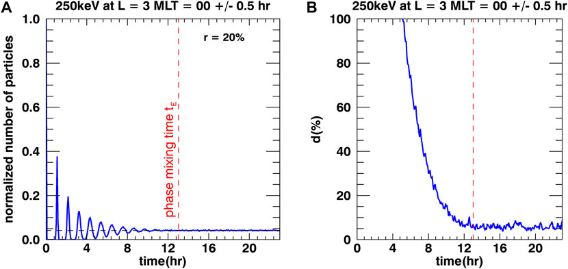
Figure 1. (A) Time evolution of the normalized number of particles situated at L = 3 and MLT = 00±0.5 h. We launch 30,000 equatorial electrons with average energy 250 keV and a standard deviation in energy of $rE/4=12.5keV$ from L = 3, MLT = 0 at t = 0. The phase mixed state is represented by a black dashed line located at $y=1/24\approx 0.04$. (B) Time evolution of the distance to the phase-mixed state, $d$ (see text for definition).

Figure 2 presents a quantification of the characteristic time for phase mixing, $t_E$, as described in Eq. 7, for equatorial electrons and two different instrument resolutions: A) high energy resolution, $r=5\%,$ and B) typical energy resolution, $r=30\%$. It shows that the characteristic time for phase mixing ranges from hours (at MeV energies in the outer belt) to several days (at low energies in the inner belt). In practice, every instrument differs in its notion of resolution, so the analysis and quantification could be redone assuming another definition for the energy resolution of the instrument, but we expect the order of magnitude to be similar.

Figure 2

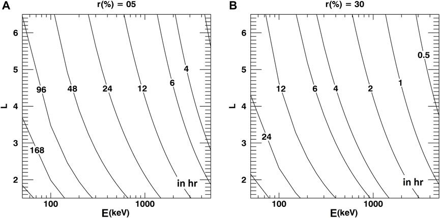
Figure 2. Characteristic time for phase mixing, in hours, due to the finite resolution in particles’ measured kinetic energy. The information is provided as a function of kinetic energy, $E$, and dipole $L$ value. The uncertainties in measured kinetic energy are described by a Gaussian distribution of standard deviation, ${\sigma }_E=rE/4$. The panels represent (A) a very high energy resolution energy instrument $\left(r=dE/E=5\%\right.$) and (B) a typical energy resolution ($\left.r=30\%\right)$

3.2 Instrumental drift phase mixing associated with the finite pitch angle resolution of the instrument

Because particles with different pitch angles have slightly different drift frequencies (Eq. 1), the finite pitch angle resolution of an instrument can also play a role in phase mixing. Since the dependence of the drift frequency on pitch angle, $F$, is relatively weak, the phase mixing process associated with this effect is expected to be less significant than the phase mixing associated with the instrument finite energy resolution. Regardless of this fact, and for completeness, a discussion of the characteristic time for phase mixing associated with the finite pitch angle resolution of the instrument is presented below.

3.2.1 Analytic expressions

Let us now consider a cluster of particles with normally distributed equatorial pitch angles, with a mean sine equal to $y_o$. Because the magnetic drift frequency is directly proportional to the function, $F$, the variance of the phase locations is directly proportional to the variance of the function, $F$, $Var\left(F\right),$ and it is straightforward to show that it evolves with time, $t$, as:

${\sigma }^2\left(t\right)={\mathrm{\Omega }}^2\frac{Var\left(F\right)}{F^2\left(y_o\right)}{t}^2(8)$

As a result, combining Eqs 3, 4, 8, the characteristic time for phase mixing associated with the instrument finite pitch angle resolution, $t_A$, is:

$t_A=\frac{\tau }{2}\frac{F\left(y_o\right)}{\sqrt{Var\left(F\right)}}(9)$

This expression is again directly proportional to the drift period, as was the case for the energy resolution mixing time (Equation 7). Its dependence on $F$ demonstrates a weak dependence of this time on the choice pitch angle, suggesting the main influence on this time will be the variance and thus the mixing time due to pitch angle aperture will be sensitive only to its resolution. We explore this briefly below.

3.2.2 Quantification

The expression 9) permits us to explore the impact of an instrument’s pitch angle resolution on the phase mixing process. To best do so, let us first consider a particularly coarse resolution where the pitch angles are normally distributed around $45°$ with an instrumental aperture of 90 $°$, meaning that 99% of the values are between $0°$ and $90°$. In this case, $F\left(y_o\right)=F\left(\sin \left(45°\right)\right)\sim 0.45$ and $\sqrt{Var\left(F\right)}\sim 0.03$, yielding the characteristic time for phase mixing associated with the instrument finite pitch angle resolution, $t_A$, to be of the order of 9 drift periods. Comparatively, this mixing time increases substantially to the order of 50 drift periods when this aperture is instead 15 $°$. We summarize this aperture effect on mixing time in Figure 3, demonstrating that the ratio between mixing time, $t_A$, and drift period, $\tau$, decays algebraically with increasing aperture size (as expected by Eq. 9).

Figure 3

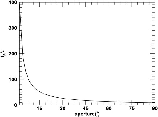
Figure 3. Ratio between the characteristic time for phase mixing associated with the finite pitch angle resolution of the instrument, $t_A$, and the drift period of the particles considered, $\tau$, as a function of instrument aperture. It is assumed that the particles have their equatorial pitch angles normally distributed around $45°$, with 99% of the pitch angles located within aperture.

Figure 3 suggests that phase mixing due to the finite pitch angle resolution of the instrument is not a significant process to account for when dealing with unidirectional measurements (with an aperture of < $10°$ ). The characteristic time for phase mixing, $t_A$, is indeed expected to be greater than 50 drift periods when the aperture is smaller than $15°$. On the other hand, phase mixing may become a significant process for wide apertures, including when dealing with omnidirectional measurements.

That said, in practice, the distribution of the drift phase locations along a drift shell may not always be very well described by a wrapped normal distribution when dealing with a population with a variety of pitch angles. Assuming a pitch angle distribution peaked around $90°$ in equatorial pitch angles for instance, the bulk of the population will also be the fastest, and the rest of the population will trail behind, creating a wrapped skewed distribution. In that case, the approach detailed in Section 7 and the criteria for phase-mixing defined in Eq. 3 need to be revised. Preliminary numerical simulations accounting for more realistic distribution functions suggest that the analytic expression for the characteristic time for phase, $t_A$, provided in Eq. 9, may actually be an underestimation of a more realistic value for the characteristic time for phase mixing associated with the instrument finite pitch angle resolution. Given these limitations, and the fact that phase mixing associated with the instrument finite pitch angle resolution appears to be a minor process in the case of unidirectional measurements (i.e., with an aperture of < $10°$), this process will be omitted thereafter, and we will focus on equatorial particles.

4 Natural drift phase mixing

In the theoretical case of a perfectly resolved instrument (measuring one exact set of kinetic energy and pitch angle values), the characteristic times for phase mixing computed in Section 3, $t_E$ and $t_A$, would both be infinitely long ($t_E=t_A=+\infty$). Yet, we still expect the drift echoes to dissipate. This is because field fluctuations naturally present in space generate perturbations in drift frequency, and ultimately, phase mixing. We present a first quantification of these characteristic times for natural drift phase mixing in the following.

4.1 Analytic expressions associated with perturbations in radial location

The omnipresence of small, slow, electric and magnetic field fluctuations means that the radial location of radiation belt particles is constantly disturbed. We show in Section 9 that the variance of the phase locations along a given drift shell is, as a first approximation for equatorial particles:

${\sigma }^2\left(t\right)=\frac{2}{3}{\left(\frac{1}{4}+\frac{3}{4{\gamma }^2}\right)}^2\frac{D_{LL}}{L^2}{\mathrm{\Omega }}^2{t}^3(10)$

where $D_{LL}$ is the radial diffusion coefficient. What is apparent at this stage is that we now have cubic, rather than quadratic, growth of the variance. This may appear unusual in the first instance but it is a consequence of the Brownian motion of particles radially contributing to the higher power of $t$. It also is the first instance of particle (radial) diffusion influencing the mixing process, and although these diffusion coefficients can be small in size they can increase by orders of magnitude thanks to magnetic activity (see Brautigam and Albert, 2000), unlike the instrumental phase mixing times. This hints to the possibility that natural mixing may dominate in most scenarios, only being eclipsed by instruments with large apertures or low energy resolutions. Combing Eqs 3, 4, 10, the characteristic time for phase mixing associated with radial diffusion, $t_F$, is:

$t_F={\left(\frac{3}{8}\right)}^{\frac{1}{3}}{\left(\frac{1}{4}+\frac{3}{4{\gamma }^2}\right)}^{-\frac{2}{3}}{\left(\frac{L^2}{D_{LL}}\right)}^{1/3}{\tau }^{\frac{2}{3}}(11)$

Thus, the characteristic time for phase mixing, $t_F$, is representative of the intensity of the field perturbations, with higher levels of radial diffusion yielding a shorter lifetime for the drift echoes. This means that, in the theoretical case of a perfectly resolved instrument (measuring one exact set of kinetic energy and pitch angle values), drift echoes’ finite lifetime could be used to quantify radial diffusion magnitude–in the absence of other significant sources of drift frequency perturbations.

4.2 Analytic expressions associated with perturbations in energy

Wave-particle interactions driving diffusion in energy and/or pitch angle, can also contribute to natural drift phase mixing. That said, because the dependence of the drift frequency in pitch angle is relatively weak (see also Section 3.2), we expect the effect of pitch angle diffusion on phase mixing time to be a secondary process. Regarding energy diffusion, we show in Section 10 that the variance of the phase locations when considering a constant energy value is, as a first approximation for equatorial particles:

${\sigma }^2\left(t\right)=\frac{1}{6}{\left(\frac{{\gamma }^2+1}{\gamma \left(\gamma +1\right)}\right)}^2\frac{D_{EE}}{E^2}{\mathrm{\Omega }}^2{t}^3(12)$

And the characteristic time for phase mixing associated with energy diffusion, $t_w$, is:

$t_W={\left(\frac{3}{2}\right)}^{\frac{1}{3}}{\left(\frac{\gamma \left(\gamma +1\right)}{{\gamma }^2+1}\right)}^{\frac{2}{3}}{\left(\frac{E^2}{D_{EE}}\right)}^{\frac{1}{3}}{\tau }^{\frac{2}{3}}(13)$

Comparing the effects of energy diffusion (Eqs 12, 13) and radial diffusion (Eqs 10, 11) on phase mixing, we see that they are of similar magnitude when $D_{EE}/E^2\approx D_{LL}/L^2$. To obtain a significant difference between the two effects, resulting in a difference of at least a factor 10 between the respective characteristic times for phase mixing, $t_W$ and $t_F$, for instance, we would need a difference of at least ${10}^3$ between $D_{EE}/E^2$ and $D_{LL}/L^2$. In the following, we will consider $D_{EE}/E^2\approx D_{LL}/L^2$ in the outer belt (L > 3), and $D_{LL}/L^2\gg D_{EE}/E^2$ in the inner belt for the sake of simplicity (e.g., Wong et al., 2024). In other words, we will consider $t_w\approx t_F$ in the outer belt, and $t_F\gg t_w$ in the inner belt.

4.3 Illustration and quantification

4.3.1 Numerical experiment using electrostatic radial diffusion

Particle injections have been observed even at very low L values (e.g., Turner et al., 2015), down to the inner belt and below (e.g., Selesnick et al., 2019). In our numerical experiment, we launched 30,000 equatorially mirroring electrons with 250 keV in the inner belt, from L = 3, MLT = 00. The particles are trapped in a magnetic dipole field and their drift motion is perturbed by a special case of random electric potential fluctuations, identical to the one described in the article by Lejosne et al. (2023). Specifically, we model the total electric potential, $V$, as the sum of a well-determined corotation potential, and some ad hoc fluctuations proportional to a random variable, $\mathrm{w}$, so that: $\mathrm{V}=-{\mathrm{\Omega }}_{\mathrm{E}}{\mathrm{B}}_{\mathrm{E}}{\mathrm{R}}_{\mathrm{E}}^3/r+\mathrm{w}\left(\mathrm{t}\right)\text{rcos}\mathrm{\phi }$, and the electric field is defined as $\mathbf{E}=-\mathbf{\nabla }\mathrm{V}.$ We assume that the variable, $\mathrm{w}$, is a piecewise constant function: the value stays constant for a set amount of time, $T=200s$, and it updates instantaneously and unpredictably at the end of every time interval. We set the standard deviation of the perturbation, $\mathrm{w}$, to a realistic value of about 0.5 mV/m. That way, the magnitude of the radial diffusion coefficient is $D_{LL}=2.2\times {10}^{-2}da{y}^{-1}$ at $L=3$, an order of magnitude that is consistent with previous estimates for radial diffusion in the inner belt and slot region (e.g., Selesnick, 2012; Obrien et al., 2016, their Figure 4). The phase mixing time provided by Eq. 11, is $t_F=23.9hr$. Figure 4 shows the phase mixing of the population, by A) representing the time evolution of the normalized number of particles at L = 3, MLT = 00 ±0.5 h and B) quantifying the maximum relative distance to the phase-mixed value. It suggests that drift phase structures could live up to a day after their generation in the Earth’s inner belt and slot region for 250 keV electrons.

Figure 4

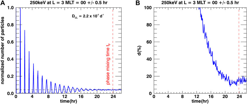
Figure 4. (A) Time evolution of the normalized number of particles situated at L = 3 and MLT = 00±0.5 h. We launch 30,000 equatorial electrons with kinetic energy 250 keV from L = 3, MLT = 00 at t = 0 and we assume a radial diffusion coefficient $D_{LL}=2.2\times {10}^{-2}da{y}^{-1}$. (B) Time evolution of the distance to the phase-mixed state, $d$ (see text for definition).

4.3.2 Quantification using electromagnetic radial diffusion

To provide a first quantification of the characteristic time for phase mixing associated with fluctuations in trapped particles’ radial location, $t_F$, we leverage the model for electromagnetic radial diffusion proposed by Brautigam and Albert (2000), in which the magnitude of radial diffusion is a function of magnetic activity, parameterized by the $Kp$ magnetic index:

$D_{LL}={10}^{-9.325+0.506\times Kp}{L}^{10}\left(da{y}^{-1}\right)(14)$

In order to get information on the range of values for the characteristic time for phase mixing associated with field fluctuations, $t_F$, we implement the formula for very quiet times (Kp = 0) and active times (Kp = 6). Figure 5 shows that phase mixing due to field fluctuations can become a significant process during active times, with a characteristic time, $t_F$, that can be smaller than the characteristic time for phase mixing associated with the instrument finite energy resolution, $t_E$ (especially in the case of high resolution instrument–Figure 2A). This reinforces the observation that the $t^3$ growth of the variance seen in Eq. 10 can have a significant role in effective MLT mixing. We can also see evidence of the role which magnetic activity plays in Figure 5B, where the mixing time decreases by around an order of magnitude in all cases. This is highly suggestive that natural mixing will be the most likely process for MLT homogenization in storm times. Regarding the first estimates provided in Figure 5, it is important to keep in mind that: a) the model by Brautigam and Albert (2000), provided in Eq. 14, was parameterized in the outer belt (interpolating experimental information provided at L = 4 and L = 6.6), and b) it is thought to underestimate radial diffusion in the inner belt (e.g., Selesnick, 2012; Obrien et al., 2016). With higher radial diffusion coefficients in the inner belt, the characteristic time for phase mixing, $t_F$, could be significantly shorter than the estimates provided in Figure 5, as is the case in Section 4.3.1 for instance.

Figure 5

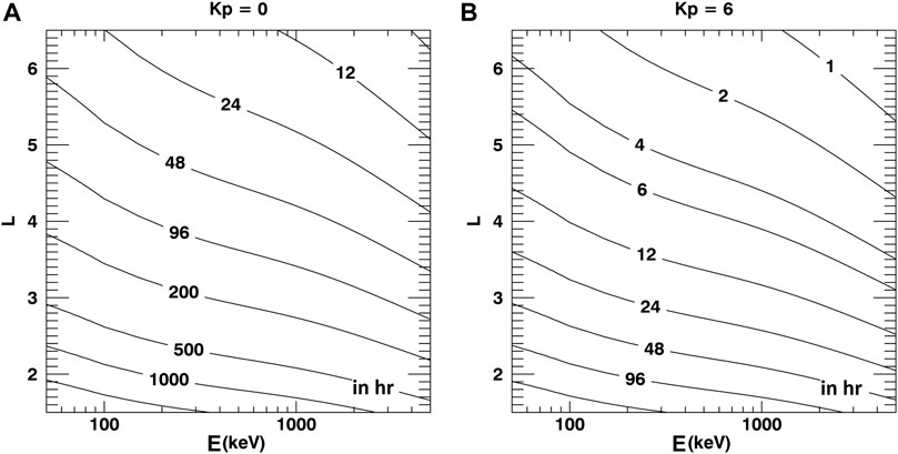
Figure 5. Characteristic time for phase mixing due to radial diffusion, $t_F$, in hours, for (A) Kp = 0 and (B) Kp = 6. The information is provided as a function of kinetic energy, $E$, and dipole $L$ value. Radial diffusion magnitude is parametrized according to Brautigam and Albert’s (2000) formula for electromagnetic radial diffusion.

5 Combining all processes

Although we have explored and characterized each mixing process individually, it is clear that in practice none of them operate in isolation. The “true” mixing time, therefore, is the cumulative effect of all operating in tandem. The focus of this section will be to use the analytic expressions for each individual process to construct an overall mixing time for the particles in MLT.

5.1 Combining instrumental and natural phase mixing processes

5.1.1 Analytic expressions

When all processes discussed in Sections 3, 4 coexist, we expect the resulting characteristic time for phase mixing, $t_T$, to be smaller than the smallest of all characteristic times for phase mixing obtained for each individual process, as discussed below.

Because the sources of perturbations are independent from each other, we can consider that the variance of the drift phase locations resulting from the combination of all instrumental and natural processes is the sum of the variances associated with each process:

${\sigma }_T^2\left(t\right)={\displaystyle \sum _i}{\sigma }_i^2\left(t\right)(15)$

where the indices $i$ label every process associated with phase-mixing–namely, the finite energy resolution of the instrument, radial diffusion, energy diffusion, and to second-order, the finite pitch angle resolution of the instrument, as well as pitch angle diffusion. In that case, a phase-mixed state is reached at a characteristic total time, $t_T$, defined as:

${\displaystyle \sum _i}{\sigma }_i^2\left(t_T\right)={\sigma }_{\mathit{lim}}^2(16)$

By definition, the characteristic time for phase mixing associated with each process, $t_i$, is such that ${\sigma }_i^2\left(t_i\right)={\sigma }_{\mathit{lim}}^2$. Thus, Eq. 16 can also be written as:

${\displaystyle \sum _i}\frac{{\sigma }_i^2\left(t_T\right)}{{\sigma }_i^2\left(t_i\right)}=1(17)$

Assuming that every variance ${\sigma }_i^2$ increases with time, t, as a power function, ${\sigma }_i^2\propto t^{n_i}$, with $n_i>0,$ we obtain that:

${\displaystyle \sum _i}{\left(\frac{t_T}{t_i}\right)}^{n_i}=1(18)$

Thus, the characteristic time for phase-mixing due to the co-existence of all processes, $t_T$, is smaller than the smallest of all the different characteristic phase-mixing times, $t_i$. This means that the mixing in the fastest variable is aided by the mixing in other processes, thus shortening the mixing process altogether.

5.1.2 Quantification and numerical illustration

5.1.2.1 Natural time for phase mixing

Let us first focus on determining the total, natural time for phase mixing in the outer belt in presence of both radial diffusion and energy diffusion, $t_o$. Following Eq. 18, it is such that:

${\left(\frac{t_o}{t_F}\right)}^3+{\left(\frac{t_o}{t_W}\right)}^3=1(19)$

Assuming $t_W=t_F$, this yields $t_o\cong 0.8t_F$. This shows that two processes of similar characteristic time for phase mixing yield a total characteristic time for phase mixing that is only slightly shorter than each individual estimate. In the inner belt, with $t_F\gg t_w$, $t_o\cong t_F.$ These results, together with the estimates for $t_F$ provided in Figure 5, suggest that the applicability of the standard, drift-averaged formulation of radial diffusion is not theoretically supported for at least an hour (up to days) after a MLT-dependent perturbation has occurred in the Earth’s radiation belts.

5.1.2.2 Total time for phase mixing resulting from the combination of observational and natural processes

Let us now consider equatorial particles, with a total phase mixing time, $t_T$, resulting from the combination of the finite energy resolution of the instrument, and radial diffusion. The characteristic time for phase-mixing associated with the finite energy resolution of the instrument, $t_E,$ provided in Eq. 7, and the characteristic time for phase-mixing due to radial diffusion, $t_F$, provided in Eq. 11, determine the total phase mixing time, $t_T$:

${\left(\frac{t_T}{t_E}\right)}^2+{\left(\frac{t_T}{t_F}\right)}^3=1(20)$

We solve numerically Eq. 20, to provide a quantification of the total characteristic time for phase mixing, leveraging the model for electromagnetic radial diffusion proposed by Brautigam and Albert (2000) to quantify $t_F$ (see also Section 4.2.2; Eq. 14). Some results are provided in Figure 6 for two different levels of magnetic activity (low magnetic activity: $Kp=0$, and high magnetic activity: $Kp=6$) and two different energy resolutions (very high energy resolution: $r=5\%$ and typical energy resolution: $r=30\%$). We note that the characteristic time for phase mixing decreases when degrading instrument resolution (i.e., increasing $r$ value), and increasing magnetic activity, as expected. That said, at a given instrument resolution, the variation with magnetic activity is more noticeable when working with a high-resolution instrument (Figures 6A, C) than with a coarse resolution (Figures 6B, D). This suggests that the characteristic time for phase mixing is dominated by instrumental effects when the energy resolution is coarse.

Figure 6

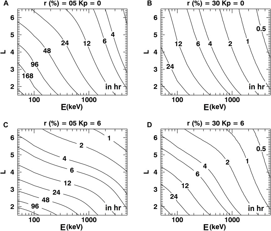
Figure 6. Characteristic time for phase mixing due to the combined effects of radial diffusion and the finite resolution in particles’ measured kinetic energy, $t_T$, in hours, for different levels of magnetic activity (top (A,B): low magnetic activity $Kp=0$, bottom (C,D): high magnetic activity $Kp=6$) and different energy resolutions (left (A,C): very high energy resolution $r=5\%$ and right (B,D): typical energy resolution $r=30\%$). The information is provided as a function of kinetic energy, $E$, and dipole $L$ value. Radial diffusion magnitude is parametrized according to Brautigam and Albert’s (2000) formula for electromagnetic radial diffusion.

Figure 7 compares and contrasts the time evolution of the same drift echo, dissipating under the effect of slow field fluctuations (radial diffusion), a) in the theoretical case of an instrument that is perfectly resolved in energy (r = 0%), as was presented in Section 4.3.1, and b) as observed by an instrument with a finite energy resolution (r = 20%). Figure 7 contributes to explaining why observations of drift phase structures have multiplied with the use of instruments with higher energy resolution (e.g., Hartinger et al., 2018). It suggests that the measured amplitude and lifetime of a drift echo are always an underestimation of the real ($r=0\%$) magnitude and lifetime of the drift echo. It also shows that the measured amplitude is always an underestimation of the initial amplitude of the drift echo. This further calls into question the applicability the standard, drift-averaged formulation of radial diffusion.

Figure 7

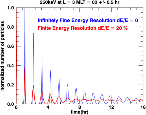
Figure 7. (In blue) Time evolution of the natural dissipation of a drift echo under radial diffusion (similar to Figure 4A)), and (in red) as viewed by an instrument with finite energy resolution ($r=dE/E=20\%$). The measured amplitude and lifetime of a drift echo (in red) are an underestimation of the real magnitude and lifetime of the drift echo (in blue).

It is interesting to compare the results of this numerical experiment in presence of both radial diffusion and finite energy resolution ($r=20\%$; $D_{LL}=2.2\times {10}^{-2}da{y}^{-1}$, red line in Figure 7) with the result of the numerical experiment in the case of drift phase mixing exclusively due to the finite energy resolution of the instrument ($r=20\%$; $D_{LL}=0da{y}^{-1}$, see blue line in Figure 1A). Both simulations provide a similar evolution for the drift echoes. With $t_E=13.02hr$ and $t_F=23.9hr$, the characteristic time for phase mixing associated with both radial diffusion and finite energy resolution is estimated to be $t_T=12.15hr$, according to Eq. 20. This estimate is comparable to $t_E$. This indicates that the evolution of the drift echoes is dominated by instrumental effect in both cases. A resolution below $r=20\%$ is required to observe the natural dissipation of drift echoes.

5.2 Instrumental calibration

In this section, we propose a way to determine the energy resolution requirements needed to guarantee that the observed dissipation of the drift echo is dominated by natural processes, rather than observational artifacts. This is of interest since the natural dissipation of drift echoes provides information on the field perturbations sampled by the particles (See Section 4.1).

In the case discussed in Section 5.1.2.2, in which total phase mixing results from the combination of radial diffusion and the finite energy resolution of the instrument, the resolution, $r_c$, for which the two processes contribute equally is such that:

${\left(\frac{t_T}{t_E\left(r_c\right)}\right)}^2={\left(\frac{t_T}{t_F}\right)}^3=\frac{1}{2}(21)$

Which occurs when

$t_E\left(r_c\right)=2^{\frac{1}{6}}{t}_F(22)$

Combining Eqs 7, 11, 22, this means that:

$r_c\cong 2{\left(\frac{\gamma \left(\gamma +1\right)}{{\gamma }^2+1}\right)\left(\frac{1}{4}+\frac{3}{{4\gamma }^2}\right)}^{\frac{2}{3}}{\left(\frac{\tau D_{LL}}{L^2}\right)}^{\frac{1}{3}}(23)$

This threshold resolution, $r_c$, can be interpreted as the minimum resolution needed to be able to detect the effect of field fluctuations in the time evolution of drift echoes. Because a higher resolution means a smaller parameter, $r$, when $r\ll r_c$ (meaning, with higher instrument resolution), we expect the evolution to be dominated by natural processes. When $r\gg r_c$ (meaning with lower instrument resolution), we expect observational limitations to be the main drivers of the drift echoes’ dissipation. In the case of our numerical experiment (250 keV at L = 3 and $D_{LL}=2.2\times {10}^{-2}da{y}^{-1}$), we find that $r_c\sim 10\%$. This explains why the evolution of the drift echoes is dominated by instrumental effects when considering $r=20\%$ (Figure 7). A general quantification of the threshold resolution, $r_c$, is provided in Figure 8, using Brautigam and Albert’s (2000) formula to parametrize electromagnetic radial diffusion as a function of the Kp index, and assuming moderate magnetic activity (Kp = 4). It shows that drift echoes’ dissipation, as observed by directional detectors with high-energy resolution ($r\sim 5\%$), could potentially be leveraged to sample field perturbations.

Figure 8

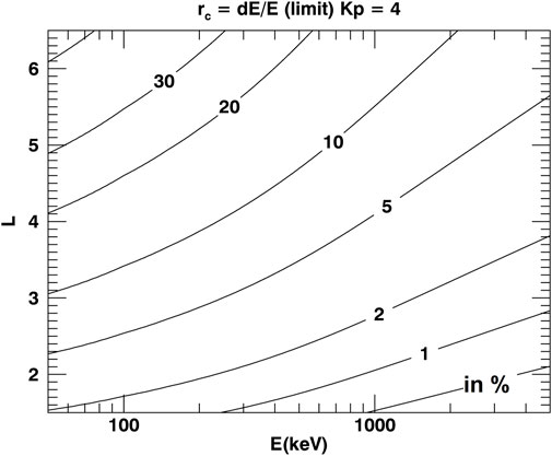
Figure 8. Minimum energy resolution required, $r_c,$ for the observed dissipation of drift echoes to be dominated by natural phase mixing, rather than observational artifacts, assuming Brautigam and Albert’s (2000) formula to parametrize electromagnetic radial diffusion and moderate magnetic activity (Kp = 4).

Therefore, this kind of analysis could be utilized to obtain the energy resolution requirements of future particle instruments. Reciprocally, when working with a known instrument resolution, the same kind of analysis can be utilized to determine the minimum magnitude of radial and/or energy diffusion needed to guarantee that the observed dissipation of drift echoes is dominated by natural phase mixing, rather than observational artifacts.

5.3 Accounting for a non-localized injection

In practice, the initial injection may not be strictly localized in MLT. In that case, the variance at the onset time, $t=0$, corresponds to the variance of the initial injection, ${\sigma }_o^2$, and the criteria for phase mixing, Eq. 3, becomes:

${\sigma }^2\left(t_{\mathit{lim}}\right)+{\sigma }_o^2={\sigma }_{\mathit{lim}}^2(24)$

which can also be written as:

$\frac{{\sigma }^2\left(t_{\mathit{lim}}\right)}{{\pi }^2}=1-\frac{{\sigma }_o^2}{{\pi }^2}(25)$

In the presence of a rather localized injection, such that ${\sigma }_o^2/{\pi }^2\ll 1$, we expect the estimates presented in this paper to not be significantly different than in the case of an initial injection peaked in MLT ($\left.{\sigma }_o^2=0\right)$.

In all cases, the estimates for the characteristic times for phase mixing at the drift scale presented in this paper can be interpreted as estimates for drift echoes’ lifetime. The presence of drift phase structures with significantly longer lifetimes could be indicative of the presence of a process maintaining phase coherence, such as drift resonance.

6 Discussion

Physics-based radiation belt models usually consist of solving a three-dimensional Fokker-Planck equation reduced to a three-dimensional fully diffusive equation (e.g., Beutier and Boscher, 1995; Subbotin and Shprits, 2009; Su et al., 2010; Tu et al., 2013; Glauert et al., 2014).

While first implemented in the case of the Earth’s radiation belts, this theoretical framework has also been applied to the radiation belts of Jupiter and Saturn (e.g., Woodfield et al., 2014; 2018; Nénon et al., 2017). All these models rely on the assumption that radiation belts are fully phase mixed at all scales, including at the drift scale.

When the theoretical framework underlying these models was first put forward (e.g., Schulz and Lanzerotti, 1974), drift echoes had already been measured by the ATS-1 satellite at the geostationary orbit (e.g., Brown, 1968; Lanzerotti et al., 1971). Yet, it was assumed that rendering MLT-dependences in radiation belts could be omitted to first order. The radial diffusion framework was indeed designed to render radiation belt dynamics on long timescales (longer than the drift period). A new generation of particle instruments, equipped with very high-energy resolution channels, highlighted the omnipresence of drift phase structures in the radiation belts. This further challenged the validity of the radial diffusion approximation to model the effect of radial transport on radiation belt dynamics, a long-standing issue in radiation belt science which is currently the object of renewed scientific interest (e.g., Riley and Wolf, 1992; Ukhorskiy et al., 2006; Ukhorskiy and Sitnov, 2008; Degeling et al., 2008; Obrien et al., 2022; Osmane et al., 2023).

The objective of this work was to quantify the time it takes for a MLT-dependent structure to phase-mix at the drift scale, that is, the time during which the (purely diffusive) radial diffusion equation does not provide an accurate description of the effect of radial transport on radiation belt intensity once a MLT-dependent perturbation has occurred. Using relatively simple first assumptions to describe instrumental response and field perturbations, we found that the time it takes for particles initially localized in local time to phase-mix is measured in hours in the Earth’s radiation belts, determining timescales during which drift remains an important driver of the dynamics. Future studies could consist of describing the effects of radial transport on radiation belt intensity using a drift-diffusion model, following an approach similar to the one presented by Lejosne et al. (2023) for instance, to determine the role played by PSD’s radial gradients (e.g., Hartinger et al., 2020) in drift echoes’ lifetimes. Several analyses of electrostatic drift echoes present in the Earth’s inner radiation belt (also known as “zebra stripes”) showed that these structures can be observed up to 14 h after generation (e.g., Lejosne and Roederer, 2016; Liu et al., 2016; Lejosne and Mozer, 2020) by the Radiation Belt Storm Probes Ion Composition Experiment (RBSPICE) instruments (Gkioulidou et al., 2023) onboard the Van Allen Probes ($r\approx 6\%$). This is consistent with the order of magnitude obtained in Section 4.3.1 (considering $t_F\ll t_E$ and $\left.t_T\approx t_F\right)$.

Regarding theoretical studies, the parameter of interest should be independent of the instrument. Thus, it is the characteristic time for natural phase mixing associated with radial diffusion and energy diffusion, $t_o$. In general, it takes hours to phase-mix in the Earth’s radiation belts, and this time is longer than the characteristic time for phase mixing due to the finite resolution of the particle instrument. This implies that non-diffusive radial transport events could have a greater and longer lasting effect on radiation belt dynamics than what was previously thought. Because the observed magnitude of drift echoes is dampened by the finite resolution of the instrument, this also means that care needs to be taken when interpreting drift echoes’ magnitude in terms of radial transport (e.g., Lejosne et al., 2022b; Obrien et al., 2022). Analysis of measured drift echoes’ magnitude should consider correcting for observational bias before interpreting drift periodic fluctuations in terms of radial transport.

The validity of the radial diffusion equation relies on the assumption that radiation belts are fully phase mixed at all scales, including at the drift scale, even though in reality, this is not necessarily the case. A more realistic implementation of the effects of radial transport on radiation belt intensity using a drift-diffusion model (e.g., Birmingham et al. (1967); Shprits et al., 2015; Lejosne and Albert, 2023) will contribute to determining how different from the radial diffusion paradigm the picture for large-scale radiation belt dynamics is when non-diffusive radial transport events are accounted for.

7 Derivation of a criteria on the variance of the drift phase locations to define a phase-mixed state

We assume that the drift phase locations of the trapped particles along the drift shell are distributed randomly, and described by a normal (Gaussian) distribution, $\mathcal{N}\left(\mu ,{\sigma }^2\right)$ on the real axis. That is, the probability distribution function is $e^{-\frac{1}{2}{\left(\frac{x-\mu }{\sigma }\right)}^2}/\sigma \sqrt{2\pi },$ with $x\mathbb{\in }\mathbb{R}$ a random drift phase location. Because the MLT locations are 2π-periodic, the resulting probability distribution is actually a wrapped normal distribution. As a result, there exists a variance limit (${\sigma }_{\mathit{lim}}^2$) for which the number of particles becomes uniform over all MLTs. To determine the value of the minimum variance, ${\sigma }_{\mathit{lim}}^2$, that defines a phase-mixed state, we compute the normalized number of particles at each hour MLT, $h$, (+/- 0.5 hr) assuming a constant average location, $\mu ,$ and different values of the variance, ${\sigma }^2$.

For illustrative purposes, we set $\mu =\pi$ (in radians), or, equivalently, noon in hour MLT. The quantity to compute is:

$n\left(h;{\sigma }^2\right)=\frac{1}{\sigma \sqrt{2\pi }}{\displaystyle \sum _{k=-\infty }^{+\infty }}{\displaystyle \underset{y=\frac{\left(h-0.5\right)\pi }{12}}{\overset{\frac{\left(h+0.5\right)\pi }{12}}{\int }}}{e}^{-\frac{1}{2}{\left(\frac{y+2k\pi -\pi }{\sigma }\right)}^2}dy(26)$

In terms of error function, with:

$\mathrm{erf}\left(z\right)=\frac{2}{\sqrt{\pi }}{\int }_0^z{e}^{-t^2}dt(27)$

The distribution, $n$, is also:

$n\left(h;{\sigma }^2\right)=\frac{1}{2}{\displaystyle \sum _{k=-\infty }^{+\infty }}\left(\mathrm{erf}\left(\frac{\frac{\left(h+0.5\right)\pi }{12}+2k\pi -\pi }{\sqrt{2}\sigma }\right)-\mathrm{erf}\left(\frac{\frac{\left(h-0.5\right)\pi }{12}+2k\pi -\pi }{\sqrt{2}\sigma }\right)\right)(28)$

Introducing the notations:

$\left\{\begin{array}{c}{\nu }_k=\left(\frac{h}{12}+2k-1\right)\frac{\pi }{\sqrt{2}\sigma }\\ \Delta \nu =\frac{1}{24}\frac{\pi }{\sqrt{2}\sigma }\end{array}\right.(29)$

yields

$n\left(h;{\sigma }^2\right)=\frac{1}{2}{\displaystyle \sum _{k=-\infty }^{+\infty }}\left(\mathrm{erf}\left({\nu }_k+\Delta \nu \right)-\mathrm{erf}\left({\nu }_k-\Delta \nu \right)\right)(30)$

When the standard deviation, $\sigma$, increases enough so that: $\Delta \nu \ll 1$, a Taylor expansion of Eq. 30 to first order in $\Delta \nu$ provides the following approximation:

$n\left(h;{\sigma }^2\right)=\frac{1}{12\sigma }\sqrt{\frac{\pi }{2}}{\displaystyle \sum _{k=-\infty }^{+\infty }}{e}^{-{\nu }_k^2}(31)$

The contribution of the $e^{-{\nu }_k^2}$ terms to the sum decreases rapidly as $\left|k\right|$ increases, indicating that the distribution converges towards a limit. It is possible to approximate the expression of the distribution function even further by conserving only the contribution of $k=0$, $k=1$, and $k=-1$, in that case:

$n\left(h;{\sigma }^2\right)\cong \frac{1}{12\sigma }\sqrt{\frac{\pi }{2}}\left(e^{-{\nu }_{-1}^2}+e^{-{\nu }_0^2}+e^{-{\nu }_1^2}\right)(32)$

For a phase-mixed distribution, we expect the resulting distribution, $n,$ to be homogenous. In other words, we expect $n=constant=1/24$ at all 24 MLT bins.

Figure 9A represents the normalized number of particles per MLT bin (with a size of one hour MLT), for three different values of the variance, ${\sigma }^2$. It shows that the distribution, $n$, tends towards a phase-mixed state as the variance increases. Figure 9B represents the maximum relative distance between the normalized number, $n$, and the phase-mixed value over all 24 MLT bins, i.e, $d=\max \left(\left|n\left(\bullet ,{\sigma }^2\right)-1/24\right|\right)\times 24,$ as a function of the value of the variance, ${\sigma }^2$. It shows that the convergence towards the phase mixed state is exponential. For the sake of simplicity, we choose ${\pi }^2$ radians as the minimum variance for which the resulting particle distribution is homogenous over all MLTs (d$<2\%$ for ${\sigma }^2<{\pi }^2$). This choice is independent of the average location, $\mu$.

Figure 9

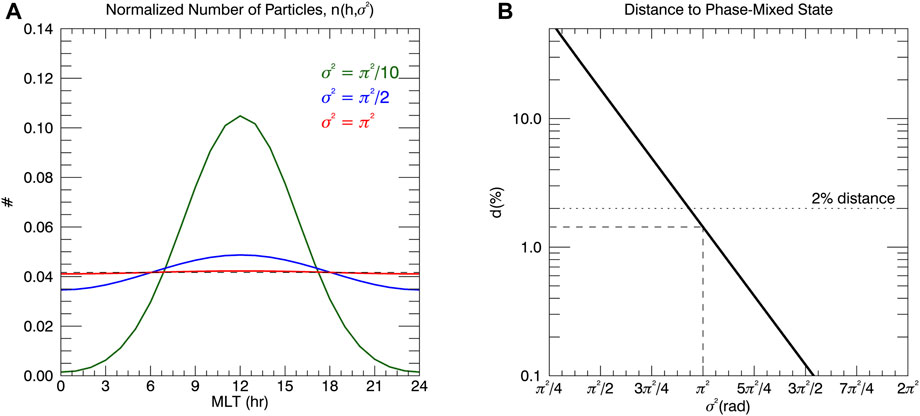
Figure 9. (A) Normalized number of particles per hour MLT, for three different values of the variance, ${\sigma }^2$, expressed in radians: (green) ${\pi }^2/10$, (blue) ${\pi }^2/2$ and (red) ${\pi }^2$, assuming a normal distribution on the real axis an average location at noon MLT. The phase-mixed state ($n=constant=1/24\sim 0.04$) is represented by a black dashed line. (B) Normalized distance to the phase-mixed state, as a function of the variance.

8 Variance of the drift phase locations due to the instrument finite energy resolution

In this section, we consider a population with kinetic energies randomly distributed around $E$, and described by a Gaussian distribution of standard deviation, ${\sigma }_E$. We show that the variance of the drift phase locations is:

${\sigma }^2\left(t\right)=\frac{{{\sigma }_E}^2}{E^2}{\left(\frac{{\gamma }^2+1}{\gamma \left(\gamma +1\right)}\right)}^2{\mathrm{\Omega }}^2{t}^2(33)$

The average phase location of the population at time, t, $\left[\phi \left(t\right)\right],$ is:

$\left[\phi \left(t\right)\right]=\frac{1}{{\sigma }_E\sqrt{2\pi }}{\int }_{u=0}^t{\int }_{\eta }\mathrm{\Omega }\left(E+\eta \right)e^{\frac{-{\eta }^2}{2{\sigma }_E^2}}d\eta du(34)$

where the integral over $\eta$ corresponds to the computation of the population’s average angular drift velocity. It accounts for the fact that the angular drift velocity depends on kinetic energy, and the population’s kinetic energies are randomly distributed around $E$. We describe the energy variable as $E+\eta$, where $\eta$ indicates the random variation from the average energy, $E$. The probability distribution function for the random energy variable, $\eta$, is a Gaussian distribution, and it is included in the averaging. The integral over $u$ from start time ($u=0$) to time $t$ converts velocity in location.

A first order Taylor expansion of $\mathrm{\Omega }\left(E+\eta \right)$, leveraging Eq. 1, is:

$\mathrm{\Omega }\left(E+\eta \right)=\mathrm{\Omega }\left(E\right)+\mathrm{\Omega }\left(E\right)\frac{\eta }{E}\left(\frac{{\gamma }^2+1}{\gamma \left(\gamma +1\right)}\right)(35)$

and Eq. 34 can be reformulated as:

$\left[\phi \left(t\right)\right]=\mathrm{\Omega }\left(E\right)t+\frac{\mathrm{\Omega }\left(E\right)}{E{\sigma }_E\sqrt{2\pi }}\left(\frac{{\gamma }^2+1}{\gamma \left(\gamma +1\right)}\right){\int }^t{\int }_{\eta }\eta e^{\frac{-{\eta }^2}{2{\sigma }_E^2}}d\eta du(36)$

Because the integral in Eq. 36 is 0, the square of the average phase location is:

${\left[\phi \left(t\right)\right]}^2={\mathrm{\Omega }}^2{t}^2(37)$

To compute the average of the square of the phase locations, we follow a similar approach. Given that:

${\mathrm{\Omega }}^2\left(E+x\right)={\mathrm{\Omega }}^2\left(E\right)+2\mathrm{\Omega }\left(E\right)\frac{\eta }{E}\left(\frac{{\gamma }^2+1}{\gamma \left(\gamma +1\right)}\right)+{\mathrm{\Omega }}^2\left(E\right)\frac{{\eta }^2}{E^2}{\left(\frac{{\gamma }^2+1}{\gamma \left(\gamma +1\right)}\right)}^2(38)$

and

$\frac{1}{{\sigma }_E\sqrt{2\pi }}\int {\eta }^2{e}^{\frac{-{\eta }^2}{2{\sigma }_E^2}}d\eta ={\sigma }_E^2(39)$

$\left[{\phi }^2\left(t\right)\right]={\mathrm{\Omega }}^2{t}^2+\frac{{\sigma }_E^2}{E^2}{\left(\frac{{\gamma }^2+1}{\gamma \left(\gamma +1\right)}\right)}^2{\mathrm{\Omega }}^2{t}^2(40)$

The result Eq. 33 is obtained by subtracting Eq. 37 from Eq. 40.

9 Variance of the drift phase locations due to field perturbations driving radial diffusion

In this section, we show that the variance of the drift phase locations associated with radial diffusion, is, to first order:

${\sigma }^2\left(t\right)=\frac{2}{3}{\left(\frac{1}{4}+\frac{3}{4{\gamma }^2}\right)}^2\frac{D_{LL}{\mathrm{\Omega }}^2}{L^2}{t}^3(41)$

for equatorial particles. For the sake of simplicity, let us first consider particles at high enough energy that ${\mathrm{\Omega }}_{\mathrm{T}}\sim \mathrm{\Omega }\gg {\mathrm{\Omega }}_E$. In the case of equatorial particles drifting in a background magnetic field,

$\mathrm{\Omega }=\frac{-3M}{\gamma q{R}_E^2{L}^2}(42)$

where $M$ is the first adiabatic invariant. Any small and slow enough (i.e., $M$ conserving) field fluctuation generating a perturbation in radial location, $\delta L$, leads to a perturbation in the angular drift velocity, $\delta \mathrm{\Omega }$, due to the direct dependence of the angular drift velocity with radial location, L, and due to the dependence of the Lorentz factor with $L$, $\gamma \left(L\right)$. Given that:

$\frac{\delta \gamma }{\gamma }=M\frac{\frac{dB}{dL}}{{{\gamma }^{2}E}_o}\delta L=\frac{-3M{B}_E\delta L}{{{\gamma }^{2}E}_o{L}^4}(43)$

$\delta \mathrm{\Omega }=\frac{-\mathrm{\Omega }}{2L}\left(1+\frac{3}{{\gamma }^2}\right)\delta L(44)$

The variation in phase, $\Delta \phi$, for a cluster of particles starting from the same location, but that are scattered (including in the radial direction) with time by random field fluctuations, is, after a time interval, $t$:

$\Delta \phi \left(t\right)={\int }_0^t\delta \mathrm{\Omega }\left(\mathrm{u}\right)\text{du}(45)$

Given Eq. 44, this is also:

$\Delta \phi \left(t\right)=\frac{-\mathrm{\Omega }}{2L}\left(1+\frac{3}{{\gamma }^2}\right){\int }_0^t\delta L\left(u\right)du(46)$

In a first approximation, $\delta L$ is a random process, which we view as a random walk. Thus, on average over many scenarios, the variation in phase is zero. For the variance, we focus on computing the average of the square of the phase variation, i.e., the statistical average of:

$\Delta {\phi }^2\left(t\right)=\frac{{\mathrm{\Omega }}^2}{4L^2}{\left(1+\frac{3}{{\gamma }^2}\right)}^2{\int }_0^t{\int }_0^t\delta L\left(u\right)\delta L\left(v\right)dudv(47)$

The statistical properties of random walks (e.g., Brockwell and Davis, 2002, p.14) are such that the autocovariance of $\delta L$ is:

$cov\left[\delta L\left(u\right),\delta L\left(v\right)\right]=2D_{LL}\min \left(u,v\right)(48)$

where $\mathit{min}\left(u,v\right)$ is the minimum of the variables $u$ and $v$.

Thus:

$Var\left[\Delta \phi \right]=\frac{{\mathrm{\Omega }}^2{D}_{LL}}{2L^2}{\left(1+\frac{3}{{\gamma }^2}\right)}^2{\int }_0^t{\int }_0^t\min \left(u,v\right)dudv(49)$

Because ${\int }_0^t{\int }_0^t\min \left(u,v\right)dudv=t^3/3$,

$Var\left[\Delta \phi \right]=\frac{{\mathrm{\Omega }}^2{D}_{LL}}{6L^2}{\left(1+\frac{3}{{\gamma }^2}\right)}^2{t}^3=\frac{8}{3}{\left(\frac{1}{4}+\frac{3}{{4\gamma }^2}\right)}^2\frac{{\mathrm{\Omega }}^2{D}_{LL}}{L^2}{t}^3(50)$

At this point in the derivation, it is important to realize that the population of particles for which we are quantifying the variance of the drift phase locations is scattering in radial distance as it is scattering in azimuthal location. To compute the characteristic time for phase mixing, it is preferable to stay on the same drift shell instead, meaning, it is preferable to focus on $L$ constant. In that case, it is important to account for the fact that there is a correlation between variation in phase, $\Delta \phi$, and variation in radial location, $\Delta L$, as quantified below.

Leveraging Eqs 46, 48, the covariance between $\Delta L$ and $\Delta \phi$ is:

$cov\left[\Delta L,\Delta \phi \right]=-2\frac{D_{LL}\mathrm{\Omega }}{L}\left(\frac{1}{4}+\frac{3}{4{\gamma }^2}\right)t^2(51)$

Given that the variance in radial location, $Var\left[\Delta L\right],$ is typically defined as:

$Var\left[\Delta L\right]=2D_{LL}t(52)$

the correlation coefficient, $\rho$, between $\Delta L$ and $\Delta \phi$ is (combining Eqs 50–52):

$\rho =\frac{cov\left[\Delta L,\Delta \phi \right]}{\sqrt{Var\left[\Delta L\right]Var\left[\Delta \phi \right]}}=\frac{-\sqrt{3}}{2}\frac{\mathrm{q}}{\left|q\right|}(53)$

And the variance of the drift phase locations at $L=constant$, ${\sigma }^2$, is related to the total variance, $Var\left[\Delta \phi \right],$ through the correlation coefficient:

${\sigma }^2=\left(1-{\rho }^2\right)Var\left[\Delta \phi \right]=\frac{Var\left[\Delta \phi \right]}{4}(54)$

This relationship can be obtained by considering the joint probability density function of a bivariate normal distribution (in $\Delta L$ and $\Delta \phi$) (e.g., Hogg and Craig, 1970, p. 111 and sq) and noting that, for $\Delta L$ set to its average value ($\left.\Delta L=0\right)$, the distribution is still normal, with a variance equal to $\left(1-{\rho }^2\right)Var\left[\Delta \phi \right]$.The combination of Eqs 50, 54 yields Eq. 41.

Small perturbations of the fields of electrostatic origin do not yield first-order perturbations in ${\mathrm{\Omega }}_E$. Thus, Eq. 41 remains valid even when considering ${\mathrm{\Omega }}_{\mathrm{T}}=\mathrm{\Omega }+{\mathrm{\Omega }}_E$, in the electrostatic case.

Finally, let us mention that this derivation relies on the standard assumption that the variance in radial location grows linearly in time (e.g., eq. (C-12)). While this is a typical assumption in radial diffusion research (e.g., Ukhorskiy et al., 2005, their Figure 5; Lejosne and Kollmann, 2020, their equation (5.19)), super-diffusive and/or sub-diffusive regimes could also exist (e.g., Desai et al., 2021; Osmane and Lejosne, 2021). Assuming different statistical models for radial transport would of course lead to different results in this analysis.

10 Variance of the drift phase locations due to field perturbations driving energy diffusion

In this section, we show that the variance of the drift phase locations associated with energy diffusion, is, to first order:

${\sigma }^2\left(t\right)=\frac{1}{6}{\left(\frac{{\gamma }^2+1}{\gamma \left(\gamma +1\right)}\right)}^2\frac{D_{EE}}{E^2}{\mathrm{\Omega }}^2{t}^3(55)$

for equatorial particles. Any perturbation in energy, $dE$, drives a perturbation in drift frequency, $\delta \mathrm{\Omega }/2\mathrm{\pi }$, given by Eq. 35:

$\delta \mathrm{\Omega }=\left(\frac{{\gamma }^2+1}{\gamma \left(\gamma +1\right)}\right)\frac{\mathrm{\Omega }}{E}dE(56)$

The variation in phase, $\Delta \phi$, for a cluster of particles starting from the same location, but that are scattered in energy with time by random field fluctuations, is, after a time interval, $t$:

$\Delta \phi \left(t\right)=\left(\frac{{\gamma }^2+1}{\gamma \left(\gamma +1\right)}\right)\frac{\mathrm{\Omega }}{E}{\int }_0^t\delta E\left(u\right)du(57)$

In a first approximation, $\delta E$ is a random process, which we view as a random walk. Thus, on average over many scenarios, the variation in phase is zero. For the variance, we focus on computing the average of the square of the phase variation, i.e., the statistical average of:

$\Delta {\phi }^2\left(t\right)=\frac{{\mathrm{\Omega }}^2}{E^2}{\left(\frac{{\gamma }^2+1}{\gamma \left(\gamma +1\right)}\right)}^2{\int }_0^t{\int }_0^t\delta E\left(u\right)\delta E\left(v\right)dudv(58)$

By definition of energy diffusion and the random walk, the autocovariance of $\delta E$ is $cov\left[\delta E\left(u\right),\delta E\left(v\right)\right]=2D_{EE}\min \left(u,v\right)$. Because ${\int }_0^t{\int }_0^t\min \left(u,v\right)dudv=t^3/3$:

$Var\left[\Delta \phi \right]=\frac{2}{3}\frac{D_{EE}}{E^2}{\left(\frac{{\gamma }^2+1}{\gamma \left(\gamma +1\right)}\right)}^2{\mathrm{\Omega }}^2{t}^3(59)$

At this point in the derivation, it is important to realize that the population of particles for which we are quantifying the variance of the drift phase locations is scattering in energy as it is scattering in azimuthal location. To compute the characteristic time for phase mixing, it is preferable to focus on a given energy, meaning, it is preferable to focus $E$ constant. In that case, it is important to account for the fact that there is a correlation between variation in phase, $\Delta \phi$, and variation in energy, $\Delta E$, as quantified below.

Leveraging Eqs 56, 57, the covariance between $\Delta E$ and $\Delta \phi$ is:

$cov\left[\Delta E,\Delta \phi \right]=\frac{D_{EE}}{E}\left(\frac{{\gamma }^2+1}{\gamma \left(\gamma +1\right)}\right)\mathrm{\Omega }{t}^2(60)$

Given that the variance in energy, $Var\left[\Delta E\right],$ is typically defined as:

$Var\left[\Delta E\right]=2D_{EE}t(61)$

The correlation coefficient, $\rho$, between $\Delta E$ and $\Delta \phi$ is, combining Eqs 59–61:

$\rho =\frac{cov\left[\Delta E,\Delta \phi \right]}{\sqrt{Var\left[\Delta E\right]Var\left[\Delta \phi \right]}}=\frac{-\sqrt{3}}{2}\frac{\mathrm{q}}{\left|q\right|}(62)$

And the variance of the drift phase locations at $E=constant$, ${\sigma }^2$, is related to the total variance, $Var\left[\Delta \phi \right],$ through the correlation coefficient:

${\sigma }^2=\left(1-{\rho }^2\right)Var\left[\Delta \phi \right]=\frac{Var\left[\Delta \phi \right]}{4}(63)$

The combination of Eqs 59, 63 yields Eq. 55.

Data availability statement

The raw data supporting the conclusion of this article will be made available by the authors, without undue reservation.

Author contributions

SL: Conceptualization, Visualization, Writing–original draft, Writing–review and editing. JA: Conceptualization, Writing–review and editing. DR: Conceptualization, Writing–review and editing.

Funding

The author(s) declare that financial support was received for the research, authorship, and/or publication of this article. SL work was performed under NASA Grant Award 80NSSC23K0518. JA was supported by NASA grant 80NSSC20K1270, AFOSR grant 22RVCOR002, and the Space Vehicles Directorate of the Air Force Research Laboratory.

Conflict of interest

The authors declare that the research was conducted in the absence of any commercial or financial relationships that could be construed as a potential conflict of interest.

Publisher’s note

All claims expressed in this article are solely those of the authors and do not necessarily represent those of their affiliated organizations, or those of the publisher, the editors and the reviewers. Any product that may be evaluated in this article, or claim that may be made by its manufacturer, is not guaranteed or endorsed by the publisher.

Author disclaimer

The views expressed are those of the authors and do not reflect the official guidance or position of the United States Government, the Department of Defense or of the United States Air Force. The appearance of external hyperlinks does not constitute endorsement by the United States Department of Defense (DoD) of the linked websites, or the information, products, or services contained therein. The DoD does not exercise any editorial, security, or other control over the information you may find at these locations.

References

Beutier, T., and Boscher, D. (1995). A three-dimensional analysis of the electron radiation belt by the Salammbô code. J. Geophys. Res. 100 (8), 14853–14861. doi:10.1029/94JA03066

CrossRef Full Text | Google Scholar

Brand, A., Allen, L., Altman, M., Hlava, M., and Scott, J. (2015). Beyond authorship: attribution, contribution, collaboration, and credit. Learn. Pub. 28, 151–155. doi:10.1087/20150211

CrossRef Full Text | Google Scholar

Brautigam, D. H., and Albert, J. M. (2000). Radial diffusion analysis of outer radiation belt electrons during the October 9, 1990, magnetic storm. J. Geophys. Res. 105 (A1), 291–309. doi:10.1029/1999JA900344

CrossRef Full Text | Google Scholar

Birmingham, T. J., Northrop, T. G., and Fälthammar, C. G. (1967). Charged particle diffusion by violation of the third adiabatic invariant. Phys. Fluids 10 (11), 2389. doi:10.1063/1.1762048

CrossRef Full Text | Google Scholar

P. J. Brockwell, and R. A. Davis (2002). Introduction to time series and forecasting (New York, NY: Springer New York).

Google Scholar

Brown, W. L. (1968). “Energetic outer-belt electrons at synchronous altitude,” in Earth's particles and fields. Editor B. M. McCormac (New York: Reinhold), 33.

Google Scholar

Degeling, A. W., Ozeke, L. G., Rankin, R., Mann, I. R., and Kabin, K. (2008). Drift resonant generation of peaked relativistic electron distributions by pc 5 ULF waves. J. Geophys. Res. 113, a–n. doi:10.1029/2007JA012411

CrossRef Full Text | Google Scholar

Desai, R. T., Eastwood, J. P., Horne, R. B., Allison, H. J., Allanson, O., Watt, C. E. J., et al. (2021). Drift orbit bifurcations and cross-field transport in the outer radiation belt: global MHD and integrated test-particle simulations. J. Geophys. Res. Space Phys. 126, e2021JA029802. doi:10.1029/2021JA029802

CrossRef Full Text | Google Scholar

Gkioulidou, M., Mitchell, D. G., Manweiler, J. W., Lanzerotti, L. J., Gerrard, A. J., Ukhorskiy, A. Y., et al. (2023). Radiation belt storm probes ion composition experiment (RBSPICE) revisited: in-flight calibrations, lessons learned and scientific advances. Space Sci. Rev. 219, 80. doi:10.1007/s11214-023-00991-x

PubMed Abstract | CrossRef Full Text | Google Scholar

Glauert, S. A., Horne, R. B., and Meredith, N. P. (2014). Three-dimensional electron radiation belt simulations using the BAS Radiation Belt Model with new diffusion models for chorus, plasmaspheric hiss, and lightning-generated whistlers. J. Geophys. Res. Space Phys. 119, 268–289. doi:10.1002/2013JA019281

CrossRef Full Text | Google Scholar

Hartinger, M. D., Claudepierre, S. G., Turner, D. L., Reeves, G. D., Breneman, A., Mann, I. R., et al. (2018). Diagnosis of ULF wave-particle interactions with megaelectron volt electrons: the importance of ultrahigh-resolution energy channels. Geophys. Res. Lett. 45 (11), 883–892. doi:10.1029/2018GL080291

CrossRef Full Text | Google Scholar

Hartinger, M. D., Reeves, G. D., Boyd, A., Henderson, M. G., Turner, D. L., Komar, C. M., et al. (2020). Why are there so few reports of high-energy electron drift resonances? Role of radial phase space density gradients. J. Geophys. Res. Space Phys. 125, e2020JA027924. doi:10.1029/2020JA027924

CrossRef Full Text | Google Scholar

Hogg, R. V., and Craig, A. T. (1970). Introduction to mathematical statistics. 3rd Edition. New York: Macmillan Publishing Company.

Google Scholar

Jaynes, A. N., Baker, D. N., Singer, H. J., Rodriguez, J. V., Loto'aniu, T. M., Ali, A. F., et al. (2015). Source and seed populations for relativistic electrons: Their roles in radiation belt changes. J. Geophys. Res. Space Physics 120, 7240–7254. doi:10.1002/2015JA021234

CrossRef Full Text | Google Scholar

Krimigis, S. M., Mitchell, D. G., Hamilton, D. C., Livi, S., Dandouras, J., Jaskulek, S., et al. (2004). Magnetosphere imaging instrument (MIMI) on the cassini mission to saturn/titan. Space Sci. Rev. 114, 233–329. doi:10.1007/s11214-004-1410-8

CrossRef Full Text | Google Scholar

Lanzerotti, L. J., Maclennan, C. G., and Robbins, M. F. (1971). Proton drift echoes in the magnetosphere. J. Geophys. Res. 76, 259. doi:10.1029/JA076i001p00259

CrossRef Full Text | Google Scholar

Lejosne, S., and Albert, J. M. (2023). Drift phase resolved diffusive radiation belt model: 1. Theoretical framework. Front. Astron. Space Sci. 10, 1200485. doi:10.3389/fspas.2023.1200485

CrossRef Full Text | Google Scholar

Lejosne, S., Albert, J. M., and Walton, S. D. (2023). Drift phase resolved diffusive radiation belt model: 2. Implementation in a case of random electric potential fluctuations. Front. Astron. Space Sci. 10, 1232512. doi:10.3389/fspas.2023.1232512

CrossRef Full Text | Google Scholar

Lejosne, S., Allison, H. J., Blum, L. W., Drozdov, A. Y., Hartinger, M. D., Hudson, M. K., et al. (2022a). Differentiating between the leading processes for electron radiation belt acceleration. Front. Astronomy Space Sci. 144. doi:10.3389/fspas.2022.896245

CrossRef Full Text | Google Scholar

Lejosne, S., Fejer, B. G., Maruyama, N., and Scherliess, L. (2022b). Radial transport of energetic electrons as determined from the zebra stripes measured in the Earth's inner belt and slot region. Front. Astronomy Space Sci. 9, 823695. doi:10.3389/fspas.2022.823695

CrossRef Full Text | Google Scholar

Lejosne, S., and Kollmann, P. (2020). Radiation belt radial diffusion at Earth and beyond. Space Sci. Rev. 216, 19. doi:10.1007/s11214-020-0642-6

CrossRef Full Text | Google Scholar

Lejosne, S., and Mozer, F. S. (2020). Experimental determination of the conditions associated with “zebra stripe” pattern generation in the earth's inner radiation belt and slot region. J. Geophys. Res. Space Phys. 125, e2020JA027889. doi:10.1029/2020JA027889

CrossRef Full Text | Google Scholar

Lejosne, S., and Roederer, J. G. (2016). The “zebra stripes”: an effect of F region zonal plasma drifts on the longitudinal distribution of radiation belt particles. J. Geophys. Res. Space Phys. 121, 507–518. doi:10.1002/2015JA021925

CrossRef Full Text | Google Scholar

Liu, Y., Zong, Q.-G., Zhou, X.-Z., Foster, J. C., and Rankin, R. (2016). Structure and evolution of electron “zebra stripes” in the inner radiation belt. J. Geophys. Res. Space Phys. 121, 4145–4157. doi:10.1002/2015JA022077

CrossRef Full Text | Google Scholar

Mitchell, D., Lanzerotti, L. J., Kim, C. K., Stokes, M., Ho, G., and Cooper, S. (2013). Radiation belt storm probes ion composition experiment (RBSPICE). Space Sci. Rev. 179, 263–308. doi:10.1007/s11214-013-9965-x

CrossRef Full Text | Google Scholar

Nénon, Q., Sicard, A., and Bourdarie, S. (2017). A new physical model of the electron radiation belts of Jupiter inside Europa's orbit. J. Geophys. Res. Space Phys. 122, 5148–5167. doi:10.1002/2017JA023893

CrossRef Full Text | Google Scholar

O'Brien, T. P., Claudepierre, S. G., Guild, T. B., Fennell, J. F., Turner, D. L., Blake, J. B., et al. (2016). Inner zone and slot electron radial diffusion revisited. Geophys. Res. Lett. 43, 7301–7310. doi:10.1002/2016GL069749

CrossRef Full Text | Google Scholar

O'Brien, T. P., Green, J. C., Halford, A. J., Kwan, B. P., Claudepierre, S. G., and Ozeke, L. G. (2022). Drift phase structure implications for radiation belt transport. J. Geophys. Res. Space Phys. 127, e2022JA030331. doi:10.1029/2022JA030331

CrossRef Full Text | Google Scholar

Osmane, A., Kilpua, E., George, H., Allanson, O., and Kalliokoski, M. (2023). Radial transport in the earth's radiation belts: linear, quasi-linear, and higher-order processes. ApJS 269, 44. doi:10.3847/1538-4365/acff6a

CrossRef Full Text | Google Scholar

Osmane, A., and Lejosne, S. (2021). Radial diffusion of planetary radiation belts’ particles by fluctuations with finite correlation time. Astrophys. J. 912, 142. doi:10.3847/1538-4357/abf04b

CrossRef Full Text | Google Scholar

Riley, P., and Wolf, R. A. (1992). Comparison of diffusion and particle drift descriptions of radial transport in the earth's inner magnetosphere. J. Geophys. Res. 97 (A11), 16865–16876. doi:10.1029/92JA01538

CrossRef Full Text | Google Scholar

Sauvaud, J. A., Moreau, T., Maggiolo, R., Treilhou, J.-P., Jacquey, C., Cros, A., et al. (2006). High-energy electron detection onboard DEMETER: the IDP spectrometer, description and first results on the inner belt. Planet. Space. Sci. 54, 502–511. doi:10.1016/j.pss.2005.10.019

CrossRef Full Text | Google Scholar

Sauvaud, J.-A., Walt, M., Delcourt, D., Benoist, C., Penou, E., Chen, Y., et al. (2013). Inner radiation belt particle acceleration and energy structuring by drift resonance with ULF waves during geomagnetic storms. J. Geophys. Res. Space Phys. 118, 1723–1736. doi:10.1002/jgra.50125

CrossRef Full Text | Google Scholar

Schulz, M. (1991). “The magnetosphere,” in Geomagnetism. Editor J. A. Jacobs (London, UK: Academic Press), 4, 87–293. cli. 2.

CrossRef Full Text | Google Scholar

Schulz, M., and Lanzerotti, L. J. (1974). Particle diffusion in the radiation belts. Berlin: Springer. doi:10.1007/978-3-642-65675-0

CrossRef Full Text | Google Scholar

Selesnick, R. S. (2012). Atmospheric scattering and decay of inner radiation belt electrons. J. Geophys. Res. 117, A08218. doi:10.1029/2012JA017793

CrossRef Full Text | Google Scholar

Selesnick, R. S., Su, Y.-J., and Sauvaud, J.-A. (2019). Energetic electrons below the inner radiation belt. J. Geophys. Res. Space Phys. 124, 5421–5440. doi:10.1029/2019JA026718

CrossRef Full Text | Google Scholar

Shprits, Y. Y., Kellerman, A. C., Drozdov, A. Y., Spence, H. E., Reeves, G. D., and Baker, D. N. (2015). Combined convective and diffusive simulations: VERB-4D comparison with 17 March 2013 Van Allen Probes observations. Geophys. Res. Lett. 42, 9600–9608. doi:10.1002/2015GL065230

CrossRef Full Text | Google Scholar

Su, Z., Xiao, F., Zheng, H., and Wang, S. (2010). Steerb: a three-dimensional code for storm-time evolution of electron radiation belt. J. Geophys. Res. 115, A09208. doi:10.1029/2009JA015210

CrossRef Full Text | Google Scholar

Subbotin, D. A., and Shprits, Y. Y. (2009). Three-dimensional modeling of the radiation belts using the Versatile Electron Radiation Belt (VERB) code. Space weather. 7, S10001. doi:10.1029/2008SW000452

CrossRef Full Text | Google Scholar

Sun, Y., Roussos, E., and Hao, Y. (2021). Saturn’s inner magnetospheric convection in the view of zebra stripe patterns in energetic electron spectra. J. Geophys. Res. Space Phys. 125 (5), e2019JA027621. doi:10.1029/2021ja029600

CrossRef Full Text | Google Scholar

Tu, W., Cunningham, G. S., Chen, Y., Henderson, M. G., Camporeale, E., and Reeves, G. D. (2013). Modeling radiation belt electron dynamics during GEM challenge intervals with the DREAM3D diffusion model. J. Geophys. Res. Space Phys. 118, 6197–6211. doi:10.1002/jgra.50560

CrossRef Full Text | Google Scholar

Turner, D. L., Claudepierre, S. G., Fennell, J. F., O'Brien, T. P., Blake, J. B., Lemon, C., et al. (2015). Energetic electron injections deep into the inner magnetosphere associated with substorm activity. Geophys. Res. Lett. 42, 2079–2087. doi:10.1002/2015GL063225

CrossRef Full Text | Google Scholar

Ukhorskiy, A., Sitnov, M., Mitchell, D., Takahashi, K., Lanzerotti, L. J., and Mauk, B. H. (2014). Rotationally driven ‘zebra stripes’ in Earth’s inner radiation belt. Nature 507, 338–340. doi:10.1038/nature13046

PubMed Abstract | CrossRef Full Text | Google Scholar

Ukhorskiy, A. Y., Anderson, B. J., Brandt, P. C., and Tsyganenko, N. A. (2006). Storm time evolution of the outer radiation belt: transport and losses. J. Geophys. Res. 111, A11S03. doi:10.1029/2006JA011690

CrossRef Full Text | Google Scholar

Ukhorskiy, A. Y., and Sitnov, M. I. (2008). Radial transport in the outer radiation belt due to global magnetospheric compressions. J. Atmos. Sol.-Terr. Phys. 70, 1714. doi:10.1016/j.jastp.2008.07.018

CrossRef Full Text | Google Scholar

Wong, J.-M., Meredith, N. P., Horne, R. B., Glauert, S. A., and Ross, J. P. J. (2024). New chorus diffusion coefficients for radiation belt modeling. J. Geophys. Res. Space Phys. 129, e2023JA031607. doi:10.1029/2023JA031607

CrossRef Full Text | Google Scholar

Woodfield, E. E., Horne, R. B., Glauert, S. A., Menietti, J. D., and Shprits, Y. Y. (2014). The origin of Jupiter's outer radiation belt. J. Geophys. Res. Space Phys. 119, 3490–3502. doi:10.1002/2014JA019891

CrossRef Full Text | Google Scholar

Woodfield, E. E., Horne, R. B., Glauert, S. A., Menietti, J. D., Shprits, Y. Y., and Kurth, W. S. (2018). Formation of electron radiation belts at Saturn by Z-mode wave acceleration. Nat. Commun. 9, 5062. doi:10.1038/s41467-018-07549-4

PubMed Abstract | CrossRef Full Text | Google Scholar

Zhao, H., Sarris, T. E., Li, X., Huckabee, I. G., Baker, D. N., Jaynes, A. J., et al. (2022). Statistics of multi-MeV electron drift-periodic flux oscillations using Van Allen Probes observations. Geophys. Res. Lett. 49, e2022GL097995. doi:10.1029/2022GL097995

CrossRef Full Text | Google Scholar

Glossary