Identification of Kelvin-Helmholtz generated vortices in magnetised fluids

The Kelvin-Helmholtz Instability (KHI), arising from velocity shear across the magnetopause, plays a significant role in the viscous-like transfer of mass, momentum, and energy from the shocked solar wind into the magnetosphere. While the KHI leads to growth of surface waves and vortices, suitable detection methods for these applicable to magnetohydrodynamics (MHD) are currently lacking. A novel method is derived based on the well-established $\lambda$-family of hydrodynamic vortex identification techniques, which define a vortex as a local minimum in an adapted pressure field. The $\mathbf{J}\times \mathbf{B}$ Lorentz force is incorporated into this method by using an effective total pressure in MHD, including both magnetic pressure and a pressure-like part of the magnetic tension derived from a Helmholtz decomposition. The ${\lambda }_{\text{MHD}}$ method is shown to comprise of four physical effects: vortical momentum, density gradients, fluid compressibility, and the rotational part of the magnetic tension. A local three-dimensional MHD simulation representative of near-flank magnetopause conditions (plasma $\beta$’s $0.5\text{–}5$ and convective Mach numbers $M_f\sim 0.4$) under northward interplanetary magnetic field (IMF) is used to validate ${\lambda }_{\text{MHD}}$. Analysis shows it correlates well with hydrodynamic vortex definitions, though the level of correlation decreases with vortex evolution. Overall, vortical momentum dominates ${\lambda }_{\text{MHD}}$ at all times. During the linear growth phase, density gradients act to oppose vortex formation. By the highly nonlinear stage, the formation of small-scale structures leads to a rising importance of the magnetic tension. Compressibility was found to be insignificant throughout. Finally, a demonstration of this method adapted to tetrahedral spacecraft observations is performed.

1 Introduction

The complex interaction between Earth’s intrinsic magnetic field and the solar wind results in a cavity called the magnetosphere, bounded by the magnetopause. Various physical processes exist which allow solar wind mass, energy, and momentum to penetrate this magnetic barrier, driving magnetospheric dynamics and also causing significant space weather effects (Buzulukova and Tsurutani, 2022). The three main mechanisms by which this penetration occurs are magnetic reconnection (Dungey, 1961), a quasi-viscous interaction (Axford and Hines, 1961; Axford, 1964), and diffusive transfer (Tsurutani and Thorne, 1982). The dominant transfer mechanism at Earth is dependent on the local Interplanetary Magnetic Field (IMF) and plasma conditions. Northward IMF conditions are conducive to viscous-like transfer, whereas southward IMF conditions enable magnetic reconnection-driven transfer to dominate. The viscous-like interaction between magnetospheric and solar wind plasma’s is predominantly driven by the Kelvin-Helmholtz instability (KHI), a fluid-like instability at interfaces with a velocity shear (Chandrasekhar, 1961), which leads to the generation and evolution of surface waves and vortices on the magnetopause (Hwang et al., 2022).

KH waves and vortices at the magnetopause form from small deformations of the boundary about equilibrium, called seed perturbations (Hasegawa et al., 2009). Because of the continuous magnetosheath flow adjacent to the magnetopause, plasma parcels closer to the boundary must move faster around these seed perturbations than ones further away. From Bernoulli’s principle, this establishes a pressure gradient which acts to further deform the magnetopause surface. These larger deformations subsequently drive greater pressure gradients and so on. Thus, in the absence of an additional force to counteract this process and stabilise the boundary, the velocity shear is KH unstable. This process occurs not only in the space plasmas at the magnetopause, it has also been observed or predicted at other planetary magnetopauses (Masters et al., 2012; Paral and Rankin, 2013; Ruhunusiri et al., 2016; Masters, 2018; Dang et al., 2022; Montgomery et al., 2023; Donaldson et al., 2024), the magnetopause of magnetised moon Ganymede (Kaweeyanun et al., 2021), comet tails (Ershkovich, 1980), and along the surface of CMEs (Nykyri and Foullon, 2013).

In the initial linear growth phase of the KHI, the deformations of the magnetopause can be described as magnetopause surface waves (MSWs) from linear MHD wave theory (Pu and Kivelson, 1983). Surface waves are magnetosonic modes which can only propagate tangentially to a boundary or surface, requiring them to have maximum amplitude at the interface and decay along the boundary normal on both sides (Kivelson and Chen, 1995). This means they can be mathematically formulated from evanescent magnetosonic waves on each side of an assumed discontinuity, tied together through boundary conditions. Surface waves are elliptically polarised with opposite polarisation on either side of the boundary, forming flow vortices centred on the interface (Dungey and Southwood, 1970).

MSWs usually originate at the near-equatorial dayside magnetopause flanks and propagate tailward due to advection by the magnetosheath flow (Song et al., 1988). As MSWs travel tailwards, their amplitudes continue to grow due to the KHI. The magnetosheath side of the interface will eventually start to carry the deformed magnetopause along with it. This results in the interface itself rolling-up into a vortex shape, which is typically seen in the instability’s nonlinear stage (Fujimoto et al., 2006). This nonlinear growth can subsequently trigger secondary processes such as vortex-induced reconnection (Nykyri and Otto, 2001; Nakamura et al., 2017; 2013), the Rayleigh-Taylor instability (Guglielmi et al., 2010), and kinetic (ion and electron) instabilities (Nykyri et al., 2006; Moore et al., 2016; 2017; Ma et al., 2021a; Nykyri et al., 2021). This makes the KHI a mechanism for cross-scale energy transfer. Understanding how the KHI’s MSWs/vortices are generated and transfer energy across the magnetopause is an active field of research that has existed since its discovery (see reviews by e.g., Zhang et al., 2022; Masson and Nykyri, 2018; Faganello and Califano, 2017; Kivelson and Chen, 1995).

By approximating the magnetopause as an unbounded tangential discontinuity between two incompressible plasmas (subscripts 1 and 2), Chandrasekhar (1961) used linear incompressible MHD theory to show that MSWs with normalised wave vector $\widehat{\mathbf{k}}$ are unstable to the KHI if Equation 1 is satisfied:

$\underset{\text{Flow}\text{Shear}\text{Driver}}{\underbrace{{\left(\widehat{\mathbf{k}}\cdot \left({\mathbf{v}}_1-{\mathbf{v}}_2\right)\right)}^2}}-\underset{\text{Density}\text{Weighting}}{\underbrace{\frac{{\rho }_1+{\rho }_2}{{\rho }_1{\rho }_2}}}\underset{\text{Magnetic}\text{Tension}\text{Stabiliser}}{\underbrace{\frac{1}{{\mu }_0}\left[{\left({\mathbf{B}}_1\cdot \widehat{\mathbf{k}}\right)}^2+{\left({\mathbf{B}}_2\cdot \widehat{\mathbf{k}}\right)}^2\right]}}>0\text{then}\text{KHI}\text{unstable.}(1)$

Here ${\mathbf{v}}_{\mathrm{1,2}}$ is the fluid velocity, ${\rho }_{\mathrm{1,2}}$ is the density, and ${\mathbf{B}}_{\mathrm{1,2}}$ is the magnetic field vector on either side of the fluid boundary. Unfortunately, this approach requires unrealistic assumptions of unbounded magnetic field lines, incompressibility, homogeneity, and an infinitesimally thin boundary layer, all of which we will show to be important along a realistic magnetopause below. While this condition has often been applied to observational case studies of the KHI to demonstrate whether the boundary is KHI unstable or not, it ought to be remembered that this condition strictly applies only at the source region of the linear stage of the KHI. Hence, when maturer vortices have developed, the data collected by a spacecraft crossing the vortex may not satisfy this condition anymore. Furthermore, it has been shown in MHD simulations that the properties (amplitude and frequency) of the KHI seed spectrum affect the growth and size of the Kelvin-Helmholtz waves–this may help explain the enhanced geo-effectiveness of solar wind structures with certain periodicities (Nykyri et al., 2017).

Equation 1 shows that wave vectors aligned with the flow shear most efficiently support the flow shear driver term of the KHI. However, this does not mean the most unstable $\widehat{\mathbf{k}}$ is necessarily aligned with the flow shear because of the second term, the stabilising effect of magnetic tension. For magnetic fields parallel to $\widehat{\mathbf{k}}$, the KHI will be suppressed by the magnetic tension if the relative speed does not exceed the root-mean-square Alfvén speed in the two media. This is intuitive–as the surface begins to deform, the frozen-in field lines will also be deformed, which magnetic tension will oppose. In contrast, magnetic fields orthogonal to $\widehat{\mathbf{k}}$ result in no curvature of field lines and hence no tension force. Thus the KHI was thought to be uninfluenced by such a magnetic field. If both magnetic fields are perpendicular to the shear flow, the most unstable $\widehat{\mathbf{k}}$ is aligned with the flow shear, whereas for magnetic fields not strictly aligned with the flow and under typical magnetopause conditions, $\widehat{\mathbf{k}}$ is most unstable perpendicular to the magnetospheric magnetic field (Southwood, 1968; Walker, 1981). Crucially, these conclusions are only true in the unbounded quasi-steady state. In reality, closed magnetospheric magnetic field lines in the vicinity of the magnetopause are necessarily bounded by the ionosphere–sometimes known as “line tying” (Miura and Kan, 1992).

The ionosphere is highly reflecting to magnetosonic modes such as surface waves, almost perfectly reflecting them and thus anchoring closed magnetic field lines in the ionosphere (Kivelson and Southwood, 1988). Thus unlike the unbounded case where a spectrum of field-aligned wavenumbers are possible, the ionospheric boundary conditions quantise the possible field-aligned wavenumbers. The result is that linear surface waves necessarily should have standing structure along the field (Chen and Hasegawa, 1974; Plaschke and Glassmeier, 2011; Archer et al., 2019; 2021). Unlike in the unbounded state, where the field lines would just move with the plasma, in the bounded state the field will now impose a magnetic tension restoring force even when it is orthogonal to the flow shear. In local simulations, this has shown to stop the vortex development if the $z$-extent around the equatorial plane is not large enough (Brackbill and Knoll, 2001; Hashimoto and Fujimoto, 2006; Takagi et al., 2006). In addition to this, it allows for the field topology to evolve. Over time, as the KHI progresses into the nonlinear stage, the bounded magnetic field can become twisted into flux ropes (Otto and Fairfield, 2000; Hwang et al., 2020; 2022) meaning that the magnetic tension will become increasingly important even when the magnetic field is orthogonal to the flow shear. This results in current sheets being generated in the mid-latitudes eventually inducing magnetic reconnection (Faganello et al., 2012; 2014). Furthermore, this twisting requires additional energy which reduces the growth rate of the KHI or stabilises the boundary entirely (Miura, 1987). This process is typical of the low-latitude flank magnetopause (e.g., Hwang et al., 2022).

So far only the incompressible regime has been considered, but plasma’s are malleable and therefore compressibility cannot be ignored. Indeed the vortices produced by the KHI act as obstacles to the driving flow, which can lead to compressions and even shocks within the plasma (e.g., Palermo et al., 2011). The fast magnetosonic convective Mach number, $M_f$, is a dimensionless number defined as a ratio of the flow speed in the obstacle frame, $u$, and the magnetosonic speed, $u_f$, such that $M_f=u/u_f$. This ratio is used to determine how compressible a flow is (Miura, 1990; Miura and Kan, 1992; Palermo et al., 2011), since the proportional change in density due to flow variations scales as $\sim M_f^2$. Values of $M_f<0.3$ are typically considered incompressible as they result in $\lesssim 10\%$ changes in density. Equation 1 shows that unstable surface waves can be generated on a incompressible infinitesimally thin tangential discontinuity when the velocity shear exceeds some critical threshold. Compressibility lowers this threshold relative to the incompressible situation and thus has a destabilising effect; the extent to which Fejer (1964), Sen (1965), and Southwood (1968) disagreed. Further to this, Sen (1965) also suggested that compressibility has both a destabilising effect on the lower critical shear flow velocity, and stabilising effect on the wave growth rate (i.e., a reduction of the growth rate) if the shear flow speed is sufficiently smaller than the magnetoacoustic speed. Pu and Kivelson (1983) coupled the results of these works by showing that there are two different modes, each with different upper and lower critical shear velocities. The modes are only unstable if the shear velocity is between the upper and lower critical shear velocity values. Pu and Kivelson (1983) show that the lower critical velocity shear of both modes is due to the stabilising effect of magnetic tension, which they show compressibility lowers for both modes. The upper critical velocity is due to a transition of the surface evanescent wave to a leaky oscillatory wave or “body wave” which carries energy away from the boundary and into the magnetosphere and magnetosheath, consequently stabilising the KHI. They show that compressibility increases the growth rate of one of the modes slightly and significantly reduces the growth rate of the other. They conclude that the impact of compressibility depends on the tangential wave vector, but generally compressibility does not significantly alter the threshold shear velocity in comparison to the incompressible limit. Crucially, these works insufficiently describe reality by approximating the magnetopause as a tangential discontinuity, making them only valid for wavelengths much larger than the boundary thickness.

Inconsistencies in growth rates at short wavelengths arise when the magnetopause’s finite thickness is ignored (Lerche, 1966), as the effects of a finite thickness stabilises the magnetopause to short wavelengths. In the compressible case KHI growth rates are reduced by the background magnetic field component parallel to the shear flow direction when using a finite thickness for the magnetopause (Ong and Roderick, 1972), agreeing with the tangential discontinuity findings of Sen (1965) and Pu and Kivelson (1983). The compressible KHI growth rates on a finite boundary were first found with linear theory by Miura and Pritchett (1982), which advanced MHD simulations of the KHI are now capable of recovering (Briard et al., 2024). As well as the growth rates, the upper and lower critical velocity conditions introduced by Pu and Kivelson (1983) are also affected when instead considering a finite boundary thickness. The lower critical shear velocity is zero when the magnetic field is orthogonal to both the shear flow and the mode’s wave vector (Miura and Kan, 1992). In addition, the upper critical velocity shear limit is removed when including an inner boundary within the magnetosphere due to the interaction of reflected waves with the magnetopause (Fujita et al., 1996). In summary, the role of compressibility is dependent on the thickness of the shear interface (Miura and Pritchett, 1982) as compressibility plays a significant role in the gradual–but not total–stabilisation of the boundary due to the finite magnetopause thickness (Miura, 1992).

Palermo et al. (2011) investigated the influence of plasma homogeneity and compressibility on the formation of KH vortices and found that compressibility, inhomogeneity, and magnetopause thickness all play a role in vortex formation and propagation and state that compressibility effects stabilise the magnetopause.

Other studies have shown that plasma inhomogeneity decreases growth rates as the gradients increase (Amerstorfer et al., 2010). Ma et al. (2024) suggest that the KHI growth rate is insensitive to the density gradient across the shear flow boundary in the compressible regime and go on to show that these variations affect the secondary processes which the KHI trigger. This further reinforces that linear incompressible theory can only approximately describe the KHI along the magnetopause. These studies suggest that magnetopause thickness, magnetic tension, and compressibility stabilise the magnetopause to the KHI, and plasma inhomogeneity destabilises it but beyond this does not affect the growth rate.

Overall, whilst this shows that the role of compressibility and magnetic tension on the KHI is a stabilising one, the significance of magnetic tension, compressibility, and density variations on vortex formation at the magnetopause is still an open question. One reason for this is because identifying MSWs and their coupled vortices using in-situ measurements or simulation is not trivial (Plaschke, 2016). Given the major role that the Kelvin-Helmhholtz instability is thought to play in the viscous-like interaction between the solar wind and magnetosphere, the ability to clearly identify the vortices produced by this process is important. This paper introduces a novel vortex identification method for Ideal MHD, based on existing methods from hydrodynamics. Current techniques, both in hydrodynamics and space plasma physics, are summarised in Section 2. Section 3 derives the new MHD-valid vortex identification method, which we call ${\lambda }_{\text{MHD}}$. We then apply the ${\lambda }_{\text{MHD}}$ method to a simple MHD simulation of the KHI in Section 4, comparing the results to previous methods and assessing the importance of different physical effects on the vortices it identifies. We also discuss potential in-situ applications.

2 Vortex identification techniques

2.1 Defining a vortex

Although a vortex is a pervasive and familiar concept which is qualitatively understood as a region of swirling fluid about some arbitrary axis line, perhaps remarkably a universally accepted mathematical vortex definition still does not exist (Jeong and Hussain, 1995; Cai et al., 2018; Yao and Hussain, 2018). To aid the discussion, it is important to understand the origins of a vortex in general. Vortices are formed when shearing momentum is redirected in some way, translating it into rotational momentum. Without an adequate restoring centripetal force, the centrifugal motion of the fluid in a vortex will tear itself apart, diffusing it. In hydrodynamics, the centripetal force that prevents this usually comes from gradients in pressure which originate from velocity gradients, following Bernoulli’s principle. This is known as cyclostrophic balance and is only true in a steady inviscid planar flow (Jeong and Hussain, 1995).

The MHD case complicates this by introducing magnetic pressure and magnetic tension forces. In MHD the restoring force will also include magnetic field contributions which are caused when the field is perturbed by the moving plasma (Collado-Vega et al., 2018). As the stress in an MHD fluid is anisotropic, due to magnetic tension introducing bias along the field direction, the consequential pressure contribution from the field will be a complex superposition of the magnetic pressure and some part of the magnetic tension (this is explored further in Section 3.1). This added complexity means that MHD requires some formal vortex definition beyond that of hydrodynamics.

2.2 Existing hydrodynamic approaches

Identifying and/or quantifying a vortex is a problem which still exists and is widely researched in the hydrodynamic community (see review by Zhang et al., 2018, and references therein). Most of these methods typically stem from the velocity gradient tensor, $\mathbf{\nabla }\mathbf{v}$ where

$\mathbf{G}=\mathbf{\nabla }\mathbf{v}=\left[\begin{array}{ccc}\hfill {\partial }_1{v}_1\hfill & \hfill {\partial }_1{v}_2\hfill & \hfill {\partial }_1{v}_3\hfill \\ \hfill {\partial }_2{v}_1\hfill & \hfill {\partial }_2{v}_2\hfill & \hfill {\partial }_2{v}_3\hfill \\ \hfill {\partial }_3{v}_1\hfill & \hfill {\partial }_3{v}_2\hfill & \hfill {\partial }_3{v}_3\hfill \end{array}\right].(2)$

One example of a popular vortex core line identification technique derived from the velocity gradient tensor is the $Q$ definition (Hunt et al., 1988). This defines a vortex as a connected fluid region with a positive second invariant of $\mathbf{\nabla }\mathbf{v}$. Finding the characteristic equation of $\mathbf{G}$ gives

$\mathrm{d}\mathrm{e}\mathrm{t}\left(\mathbf{G}-\lambda \mathbf{I}\right)={\lambda }^3-P{\lambda }^2+Q\lambda -R=0(3)$

where the first, second, and third invariants of $\mathbf{G}$ are defined respectively as

$P=\mathrm{T}\mathrm{r}\left(\mathbf{G}\right);Q=\frac{1}{2}\left[\mathrm{T}\mathrm{r}{\left(\mathbf{G}\right)}^2-\mathrm{T}\mathrm{r}\left({\mathbf{G}}^2\right)\right];R=\mathrm{d}\mathrm{e}\mathrm{t}\left(\mathbf{G}\right).(4)$

For an incompressible fluid $\left(\nabla \cdot \mathbf{v}=\mathrm{T}\mathrm{r}\left(\mathbf{G}\right)=0\right)$, the $Q$ criterion is equivalent to a region where the magnitude of the rotation rate tensor, $\mathbf{\Omega }=\frac{1}{2}\left({\mathbf{G}}^T-\mathbf{G}\right)$, is larger than the magnitude of the strain-rate tensor, $\mathbf{S}=\frac{1}{2}\left({\mathbf{G}}^T+\mathbf{G}\right)$. This is expressed as $\left(\Vert \mathbf{\Omega }{\Vert }_F^2-\Vert \mathbf{S}{\Vert }_F^2\right)$ where $\Vert \cdot {\Vert }_F$ is the Frobenius norm given by $\Vert \underline{\mathbf{X}}{\Vert }_F=\sqrt{{\sum }_{i=1}^n{\sum }_{j=1}^m{X}_{ij}^2}$. Due to its simplicity, this strictly incompressible definition of $Q$ is usually applied, even when dealing with compressible fluids.

Another popular vortex core line identification technique derived from the velocity gradient tensor, and based on locating local pressure minima, is the ${\lambda }_2$ definition (Jeong and Hussain, 1995). The technique starts with the Navier-Stokes momentum equation and derives the pressure Hessian, containing local pressure extrema information. After discarding unsteady irrotational straining and viscous effects, which are unrelated to vortical motion, this becomes

${\partial }_i{\partial }_j{P}_{\text{adp}}=S_{ik}{S}_{kj}+{\mathrm{\Omega }}_{ik}{\mathrm{\Omega }}_{kj},(5)$

where $P_{\text{adp}}$ is the adapted pressure (pressure with the unsteady irrotational straining and viscous effects removed). An adapted pressure minimum in some plane requires, through a second partial derivative test on $P_{\text{adp}}$, two negative eigenvalues of ${\mathbf{S}}^2+{\mathbf{\Omega }}^2$. Hence a vortex core in this method is defined as a connected region which satisfies this condition. This can be simplified by sorting the eigenvalues in descending order: ${\lambda }_1>{\lambda }_2>{\lambda }_3$ and stating a vortex occurs where ${\lambda }_2<0$ (a step-by-step derivation can be found in the appendix of Cucitore et al., 1999). ${\lambda }_2$ can be interpreted as identifying a local pressure minima in some arbitrary intersecting plane. Due to how the value is constructed, the magnitude of the parameters does not have any physical significance except for comparison to other values of itself. Cucitore et al. (1999) show that the ${\lambda }_2$ method is a requirement of some measure of the rotation rate prevailing over some measure of the strain rate, implying that ${\lambda }_2$ and $Q$ are comparable.

Both of these criteria are only valid for homogeneous and incompressible hydrodynamic fluids. In addition, as they both only use the velocity vector field, they are ignorant to the momentum they represent. Extensions to these techniques do exist which provide weighting dependent on momentum. The simplest is weighted-${\lambda }_2$ (Yao and Hussain, 2018) (denoted as $\overline{{\lambda }_2}$ herein) which is identical to ${\lambda }_2$ but weights Equation 5 by density. This results in a shifting of power from high velocity vortices to high momentum vortices. A further extension is known as ${\lambda }_{\rho }$ (Yao and Hussain, 2018) which extends ${\lambda }_2$ to be valid for compressible, inhomogeneous hydrodynamic fluids. This is achieved by using the symmetric part to the tensor product of the momentum gradient tensor, $\mathbf{\nabla }(\rho \mathbf{v})$, and the velocity gradient tensor, $\mathbf{\nabla }\mathbf{v}$, along with the symmetric part of the momentum compressibility gradient tensor, $\mathbf{\nabla }\left[\left(\mathbf{\nabla }\cdot \mathbf{v}\right)\rho \mathbf{v}\right]$. ${\lambda }_{\rho }$ can be broken into three parts which represent the vortical momentum, the fluid compressibility, and the density gradients. If the definition is applied to an incompressible and homogeneous fluid then it reduces to $\overline{{\lambda }_2}$. A useful feature of the $Q$ and $\lambda$-family of techniques is that they are Galilean invariant (Jeong and Hussain, 1995), meaning the methods are consistent across all inertial frames of reference.

2.3 Current approaches to vortex identification at the magnetopause

Typically, MSWs due to the KHI at the magnetopause are identified in-situ by using hodograms to show quasi-periodic fluctuations of the magnetopause surface passing over spacecraft (Hasegawa et al., 2004). This method is deficient if only single spacecraft measurements are used as it can be difficult to characterise structure size (Hasegawa et al., 2004). As well as this, the method cannot identify magnetopause vortex structures (Cai et al., 2018). Vortical patterns will be present in the data from both surface roll-up and the boundary adjacent vortices the waves generate in the boundary-adjacent flow. It is important to be able to distinguish between them as surface roll-ups only occur in the nonlinear stages of the KHI but boundary-adjacent vortical flow can occur at any stage (Chandrasekhar, 1961; Hwang et al., 2022). This makes identifying vortices and their coupled surface waves two different problems.

Numerous vortex identification techniques applicable to the magnetopause have been developed but all have deficiencies (see review by Hasegawa, 2012). For example, a sensible starting place for vortex identification would be using the vorticity vector. However, at shear boundary regions vorticity is high even in the absence of any rotating flows, meaning that it is not suitable for KH vortex identification. Takagi et al. (2006) suggested using low-density plasma moving faster than the magnetosheath plasma to detect surface roll-ups. However, Plaschke et al. (2014) showed that this signature is not unique to surface roll-ups due to the plasma depletion layer and vortices from MSWs providing false-positives. Alternatively, based on a hybrid Vlasov simulation of the KHI, Settino et al. (2021) suggest kinetic signatures such as ion non-Maxwellianity, total current density, temperature anisotropy, agyrotropy, and magnetic field gradients might serve as proxies for KH-vortices.

Another popular method used for both simulation and in-situ analysis investigates local total pressure minima, where the total pressure is the sum of thermal and magnetic pressures (Nykyri et al., 2017; Rice et al., 2022). Pressure minima are coupled to vortices due to Bernoulli’s principle as discussed above. This approach, and using the vorticity vector, typically fails when fluctuations are large or if other physical processes which can interfere with the dynamics of the KHI (e.g., reconnection) are taking place (Settino et al., 2021). Other drawbacks of local pressure minima arise due to the vortex not containing a three-dimensional pressure minima and also pressure minima not always being associated with vortices as other physical process can create them.

The simpler hydrodynamic vortex identification techniques ($Q$ and ${\lambda }_2$) have also been used to study the KHI at Earth’s magnetopause, though this is only possible for multi-point analysis due to the necessity of calculating gradients (Settino et al., 2021). Cai et al. (2018) used data from the Cluster Mission (Escoubet et al., 2001) to identify vortical structures at Earth’s magnetopause. They applied the method to magnetic field data rather than the velocity data, assuming these vary similarly via the frozen-in flux theorem. They conclude that $Q$ is easy to implement but imprecise and that ${\lambda }_2$ is more precise but does not provide geometric information about the vortex core. These results agree with a different study performed by Collado-Vega et al. (2018) who investigated the effectiveness of $Q$ and ${\lambda }_2$ in identifying vortices in a 3-dimensional BATS-R-US global MHD magnetosphere simulation (Tóth et al., 2005). They state that neither method is immune to false identifications and conclude by stating that incorporating the effects of the magnetic field will likely increase the scientific yield. Since both techniques derive from hydrodynamics, this can only be done by deriving the equivalent to the $\lambda$-family of methods from the MHD equations.

3 The $\lambda$ method for ideal MHD

3.1 MHD effective pressure

The $\lambda$-family of definitions all work by using a second partial derivative test on some adapted pressure Hessian to find local pressure minima. Local pressure minima here refers to a minima in pressure in a plane, not a three dimensional minima as some vortices only have minima in a plane perpendicular to a vortex axis rather than a three dimensional minima (e.g., Burgers vortex). In the case of hydrodynamics without any external forces, the only inviscid force acting on the fluid arises from thermal pressure gradients. Thus thermal pressure is the field used, adapted by discarding any contributions which cause pressure minima without being associated with vortical flow, e.g., sink flow (Jeong and Hussain, 1995). However, in MHD the plasma is also subject to magnetic pressure and magnetic tension forces. The total pressure generally used in ideal MHD is the sum of magnetic pressure, $P_{\text{mag}}=B^2/(2{\mu }_0)$, and thermal pressure, $P_{\text{therm}}=n{k}_{B}T$. However this does not necessarily describe all the pressure-like forces on the plasma–those which can be expressed as an irrotational field $-(\mathbf{\nabla }P)$. The magnetic tension $\mathbf{B}\cdot \nabla \mathbf{B}/{\mu }_0$ may also have a pressure-like part to it. One example of this is the magnetic dipole, which is a current- and force-free magnetic field. Since this exhibits magnetic pressure gradients, these must be completely cancelled by magnetic tension forces; thus tension can in part contribute to the total of pressure-like forces in ideal MHD. In an alternative case where current is induced, such as in a field aligned current, the magnetic tension will be a highly rotational field as stress is transmitted along the field. This highlights that in a dynamic environment such as KH vortices, the magnetic tension will be composed of both rotational and irrotational components.

The fundamental theorem of vector calculus states that any vector field, which exists in the domain $V$ and is twice continuously differentiable inside $V$, can be decomposed into the sum of a curl-free (irrotational, $-\mathbf{\nabla }P$), and divergence-free (rotational $\mathbf{\nabla }\times \mathbf{U}$), field. This is also known as a Helmholtz decomposition. Applied to the magnetic tension this gives

$\mathit{\tau }=-\mathbf{\nabla }{P}_{\text{ten}}+\mathbf{\nabla }\times \mathbf{U}={\mathit{\tau }}_{\text{\hspace{0.17em}irr}}+{\mathit{\tau }}_{\text{\hspace{0.17em}rot}},(6)$

where $P_{\text{ten}}$ is the pressure field associated with the irrotational part of the tension force and $\mathbf{U}$ is the vector potential field describing the rotational part to the tension. The Helmholtz decomposition allows for an effective total pressure field in MHD to be defined as the sum of thermal pressure, magnetic pressure, and the pressure-like part of the tension:

$P_{\text{eff}}=n{k}_{B}T+\frac{B^2}{2{\mu }_0}+P_{\text{ten}}=P_{\text{therm}}+P_{\text{mag}}+P_{\text{ten}}.(7)$

A general solution to Equation 6 can be derived so that $P_{\text{ten}}$ can be investigated

$\begin{array}{ll}\hfill \mathit{\tau }\left(\mathbf{r}\right)=& -\mathbf{\nabla }\underset{P_{\text{ten}}\left(\mathbf{r}\right)}{\underbrace{\left(\frac{1}{4\pi }{\int }_V\frac{{\mathbf{\nabla }}^{\prime }\cdot \mathit{\tau }\left({\mathbf{r}}^{\prime }\right)}{\left|\mathbf{r}-{\mathbf{r}}^{\prime }\right|}\mathrm{d}{V}^{\prime }-\frac{1}{4\pi }{\oint }_S{\widehat{\mathbf{n}}}^{\prime }\cdot \frac{\mathit{\tau }\left({\mathbf{r}}^{\prime }\right)}{\left|\mathbf{r}-{\mathbf{r}}^{\prime }\right|}\mathrm{d}{S}^{\prime }\right)}}\hfill \\ \hfill & +\mathbf{\nabla }\times \underset{\mathbf{U}\left(\mathbf{r}\right)}{\underbrace{\left(\frac{1}{4\pi }{\int }_V\frac{{\mathbf{\nabla }}^{\prime }\times \mathit{\tau }\left({\mathbf{r}}^{\prime }\right)}{\left|\mathbf{r}-{\mathbf{r}}^{\prime }\right|}\mathrm{d}{V}^{\prime }-\frac{1}{4\pi }{\oint }_S{\widehat{\mathbf{n}}}^{\prime }\times \frac{\mathit{\tau }\left({\mathbf{r}}^{\prime }\right)}{\left|\mathbf{r}-{\mathbf{r}}^{\prime }\right|}\mathrm{d}{S}^{\prime }\right)}}.\hfill \end{array}(\mathrm{8a})$

$=-\mathbf{\nabla }{P}_{\text{ten}}+\mathbf{\nabla }\times \mathbf{U}(\mathrm{8b})$

where $S$ is the enclosing surface of $V$.

Axiomatically, $P_{\text{ten}}$ and $\mathbf{U}$ are not unique. Any arbitrary constant scalar can be added to $P_{\text{ten}}$ to provide the same distinct ${\mathit{\tau }}_{\text{\hspace{0.17em}irr}}=-\mathbf{\nabla }{P}_{\text{ten}}$ solution. Similarly, any arbitrary gradient field can be added to $\mathbf{U}$ to give the same unique solution to ${\mathit{\tau }}_{\text{\hspace{0.17em}rot}}=\mathbf{\nabla }\times \mathbf{U}$. As the effective pressure itself is not directly required in $\lambda$-family methods, only its Hessian, this gauge freedom is unimportant here.

Computationally, it is more efficient to perform the Helmholtz decomposition in Fourier space

$\mathit{\tau }=\iiint \widehat{\mathit{\tau }}\left(\mathbf{k}\right)e^{i\mathbf{k}\cdot \mathbf{r}}d{V}_k,(9)$

where $\widehat{\mathit{\tau }}$ denotes the Fourier Transform of the magnetic tension. In an unbounded domain this requires that the tension decays faster than $1/r$. By splitting the tension’s Fourier transform $\widehat{\mathit{\tau }}(\mathbf{k})$ into its components parallel and perpendicular to $\mathbf{k}$

${\widehat{\mathit{\tau }}}_{\Vert }\left(\mathbf{k}\right)=\frac{\mathbf{k}\cdot \widehat{\mathit{\tau }}\left(\mathbf{k}\right)}{|\mathbf{k}{|}^2}\mathbf{k},(10)$

${\widehat{\mathit{\tau }}}_{\perp }\left(\mathbf{k}\right)=-\mathbf{k}\times \frac{\mathbf{k}\times \widehat{\mathit{\tau }}\left(\mathbf{k}\right)}{|\mathbf{k}{|}^2},(11)$

it can be seen that

$\widehat{\mathit{\tau }}\left(\mathbf{k}\right)={\widehat{\mathit{\tau }}}_{\Vert }\left(\mathbf{k}\right)+{\widehat{\mathit{\tau }}}_{\perp }\left(\mathbf{k}\right)(\mathrm{12a})$

$=-i\mathbf{k}\frac{i\mathbf{k}\cdot \widehat{\mathit{\tau }}\left(\mathbf{k}\right)}{|\mathbf{k}{|}^2}+i\mathbf{k}\times \frac{i\mathbf{k}\times \widehat{\mathit{\tau }}\left(\mathbf{k}\right)}{|\mathbf{k}{|}^2}(\mathrm{12b})$

$=-i\mathbf{k}{\widehat{P}}_{\text{ten}}\left(\mathbf{k}\right)+i\mathbf{k}\times \widehat{\mathbf{U}}\left(\mathbf{k}\right)(\mathrm{12c})$

where the Fourier Transforms of the scalar field $P_{\text{ten}}$ and the vector field $\mathbf{U}$ are defined as

${\widehat{P}}_{\text{ten}}\left(\mathbf{k}\right)=i\frac{\mathbf{k}\cdot \widehat{\mathit{\tau }}\left(\mathbf{k}\right)}{|\mathbf{k}{|}^2},(13)$

$\widehat{\mathbf{U}}\left(\mathbf{k}\right)=i\frac{\mathbf{k}\times \widehat{\mathit{\tau }}\left(\mathbf{k}\right)}{|\mathbf{k}{|}^2}.(14)$

Substituting into Equation 9 demonstrates this provides the Helmholtz decomposition

$\mathit{\tau }=\underset{-\nabla P_{\text{ten}}}{\underbrace{\iiint -i\mathbf{k}{\widehat{P}}_{\text{ten}}\left(\mathbf{k}\right)e^{i\mathbf{k}\cdot \mathbf{r}}d{V}_k}}+\underset{\nabla \times \mathbf{U}}{\underbrace{\iiint i\mathbf{k}\times \widehat{\mathbf{U}}\left(\mathbf{k}\right)e^{i\mathbf{k}\cdot \mathbf{r}}d{V}_k}},(15)$

since in Fourier space $\nabla \to i\mathbf{k}$. The Fourier method has been used to perform the decomposition seen in the following section.

3.2 ${\lambda }_{\mathrm{MHD}}$ derivation

Here we derive a $\lambda$-family vortex definition applicable to ideal MHD, which we call ${\lambda }_{\text{MHD}}$. The derivation closely follows that of ${\lambda }_{\rho }$ found in Yao and Hussain (2018). The aim is to find the Hessian of the MHD effective pressure defined in Section 3.1 so that a second partial derivative test can be performed on it to identify local pressure minima. Gravitational effects are assumed to be negligible. We neglect viscous effects in the derivation below due to space plasma being collisionless. However, this definition is valid for a viscous ideal MHD fluid as a viscosity term in the pressure Hessian is neglected as viscosity can provide centripetal forces (e.g., Kármán’s viscous pump) and remove the pressure minima in the fluid. Neglecting this term allows for the method to be able to successfully identify a vortex even when pressure-minima are not providing the centripetal restoring force (see Jeong and Hussain, 1995; Yao and Hussain, 2018, for further description of the viscous case in hydrodynamics).

The derivation starts with the ideal MHD Cauchy-Momentum equation, where the Helmholtz decomposition of the magnetic tension has been performed

$\frac{\partial }{\partial t}\left(\rho \mathbf{v}\right)+\mathbf{\nabla }\cdot \left(\rho \mathbf{v}\mathbf{v}\right)=-\mathbf{\nabla }{P}_{\text{eff}}+{\mathit{\tau }}_{\text{rot}}.(16)$

Rewriting this in tensor notation (using the Einstein summation convention) for component $i$ and taking the gradient in coordinate $j$,

${\partial }_t{\partial }_j\left(\rho v_i\right)+{\partial }_j{\partial }_k\left(\rho v_i{v}_k\right)=-{\partial }_j{\partial }_i{P}_{\text{\hspace{0.17em}eff}}+{\partial }_j{\tau }_{i\text{\hspace{0.17em}rot}}.(17)$

Apply the chain rule twice

$\begin{array}{c}{\partial }_t{\partial }_j\left(\rho v_i\right)+{\partial }_j{v}_k{\partial }_k\left(\rho v_i\right)+v_k{\partial }_k{\partial }_j\left(\rho v_i\right)\hfill \\ +{\partial }_j\left(\rho v_i\right){\partial }_k{v}_k+\left(\rho v_i\right){\partial }_k{\partial }_j{v}_k=-{\partial }_j{\partial }_i{P}_{\text{\hspace{0.17em}eff}}+{\partial }_j{\tau }_{i\text{\hspace{0.17em}rot}}.\hfill \end{array}(18)$

Using the definition of the material derivative $\frac{D}{Dt}={\partial }_t+v_k{\partial }_k$ this can be simplified to

$\begin{array}{c}\hfill \frac{D}{Dt}\left({\partial }_j\left(\rho v_i\right)\right)+{\partial }_j{v}_k{\partial }_k\left(\rho v_i\right)+{\partial }_j\left(\left(\rho v_i\right){\partial }_k{v}_k\right)=-{\partial }_j{\partial }_i{P}_{\text{\hspace{0.17em}eff}}+{\partial }_j{\tau }_{i\text{\hspace{0.17em}rot}}.\end{array}(19)$

Taking the symmetric part of Equation 19 by applying to each tensor $A_{ij}$ the symmetric operator $1/2\left(A_{ij}+A_{ji}\right)$

$\begin{array}{cc}\hfill & \frac{D}{Dt}\left(\frac{1}{2}\left({\partial }_j\left(\rho v_i\right)+{\partial }_i\left(\rho v_j\right)\right)\right)+\frac{1}{2}\left({\partial }_j{v}_k{\partial }_k\left(\rho v_i\right)+{\partial }_i{v}_k{\partial }_k\left(\rho v_j\right)\right)\hfill \\ \hfill & +\frac{1}{2}\left({\partial }_j\left(\left(\rho v_i\right){\partial }_k{v}_k\right)+{\partial }_i\left(\left(\rho v_j\right){\partial }_k{v}_k\right)\right)=-{\partial }_j{\partial }_i{P}_{\text{\hspace{0.17em}eff}}+\frac{1}{2}\left({\partial }_j{\tau }_{i\text{\hspace{0.17em}rot}}+{\partial }_i{\tau }_{j\text{\hspace{0.17em}rot}}\right).\hfill \end{array}(20)$

Substitute in the symmetric, $S_{ij}=1/2\left({\partial }_j{v}_i+{\partial }_i{v}_j\right)$, and anti-symmetric, ${\mathrm{\Omega }}_{ij}=1/2\left({\partial }_j{v}_i-{\partial }_i{v}_j\right)$, parts of the velocity gradient tensor

$\begin{array}{cc}\hfill & \frac{D}{Dt}\left(\frac{1}{2}\left({\partial }_j\left(\rho v_i\right)+{\partial }_i\left(\rho v_j\right)\right)\right)+\rho \left(S_{ik}{S}_{kj}+{\mathrm{\Omega }}_{ik}{\mathrm{\Omega }}_{kj}\right)+\frac{{\partial }_k\rho }{2}\left(v_i{\partial }_j{v}_k+v_j{\partial }_i{v}_k\right)\hfill \\ \hfill & +\frac{1}{2}\left({\partial }_j\left(\left(\rho v_i\right){\partial }_k{v}_k\right)+{\partial }_i\left(\left(\rho v_j\right){\partial }_k{v}_k\right)\right)=-{\partial }_j{\partial }_i{P}_{\text{\hspace{0.17em}eff}}+\frac{1}{2}\left({\partial }_j{\tau }_{i\text{\hspace{0.17em}rot}}+{\partial }_i{\tau }_{j\text{\hspace{0.17em}rot}}\right).\hfill \end{array}(21)$

The effective pressure Hessian (denoted $\mathbf{H}$) can now be written as,

${-H}_{ij}=-{\partial }_j{\partial }_i{P}_{\text{eff}}=E_{ij}+M_{ij}+D_{ij}+C_{ij}+T_{ij}.(\mathrm{22a})$

Where each term represents a different physical property:

$\text{Unsteady\hspace{0.17em}Strain:\hspace{0.17em}}{E}_{ij}=\frac{D}{Dt}\left(\frac{1}{2}\left({\partial }_j\left(\rho v_i\right)+{\partial }_i\left(\rho v_j\right)\right)\right),(\mathrm{22b})$

$\text{Vortical\hspace{0.17em}Momentum:\hspace{0.17em}}{M}_{ij}=\rho \left(S_{ik}{S}_{kj}+{\mathrm{\Omega }}_{ik}{\mathrm{\Omega }}_{kj}\right),(\mathrm{22c})$

$\text{Density\hspace{0.17em}Gradients:\hspace{0.17em}}{D}_{ij}=\frac{{\partial }_k\rho }{2}\left(v_i{\partial }_j{v}_k+v_j{\partial }_i{v}_k\right),(\mathrm{22d})$

$\text{Compressibility:\hspace{0.17em}}{C}_{ij}=\frac{1}{2}\left({\partial }_j\left(\left(\rho v_i\right){\partial }_k{v}_k\right)+{\partial }_i\left(\left(\rho v_j\right){\partial }_k{v}_k\right)\right),(22e)$

$\text{Rotational\hspace{0.17em}Magnetic\hspace{0.17em}Tension:\hspace{0.17em}}{T}_{ij}=-\frac{1}{2}\left({\partial }_j{\tau }_{i\text{\hspace{0.17em}rot}}+{\partial }_i{\tau }_{j\text{\hspace{0.17em}rot}}\right).(\mathrm{22f})$

As discussed by Jeong and Hussain (1995) and Yao and Hussain (2018), there is an inconsistency between the existence of a pressure minimum and a vortex core in Equation (22a). Simply finding a local pressure minimum is not sufficient in identifying a vortex core as unsteady irrotational motion can cause pressure minima in a fluid without vortical flow as a consequence of unsteady strain in the fluid. In the example of a surface wave in an incompressible isothermal hydrodynamic fluid, a vortex would not be identifiable in pressure alone as there would not be a pressure minimum despite vortical flow being present. However, removing the unsteady strain provides the minimum needed in the adapted pressure Hessian to allow for vortex identification in this case. Choosing to neglect the unsteady strain effect in Equation 22a completes the derivation,

$-\mathbf{H}=\mathbf{M}+\mathbf{D}+\mathbf{C}+\mathbf{T}.(23)$

Equation 23 outlines that only contributions from $\mathbf{M}+\mathbf{D}+\mathbf{C}+\mathbf{T}$ are required to identify a pressure minimum in a plane, which requires two positive eigenvalues of the pressure Hessian tensor (Jeong and Hussain, 1995; Yao and Hussain, 2018). Consequently, ${\lambda }_{\text{MHD}}$ defines a vortex as a connected region with two negative eigenvalues of $\mathbf{M}+\mathbf{D}+\mathbf{C}+\mathbf{T}$. Since this tensor is real and symmetric, it has real eigenvalues only. Thus if its eigenvalues ${\lambda }_1>{\lambda }_2>{\lambda }_3$, then ${\lambda }_{\text{MHD}}$ is equivalent to the requirement that ${\lambda }_2<0$ within the vortex core.

In summary, ${\lambda }_{\text{MHD}}$ adds a correction term to ${\lambda }_{\rho }$ which extends its usage to a magnetised ideal MHD fluid. ${\lambda }_{\text{MHD}}$ is constructed of four terms which each represent different physical effects believed to affect the formation of the vortices such as in the KHI: vortical momentum $(\mathbf{M})$, density gradients $(\mathbf{D})$, fluid compressibility $(\mathbf{C})$, and rotational magnetic tension $(\mathbf{T})$.

4 Application to local MHD simulation

To demonstrate ${\lambda }_{\text{MHD}}$ and its potential usage in identifying MSWs and vortices at the magnetopause due to KHI, we apply it to data from a local MHD simulation of the KHI. Here local refers to the simulation being a simplified and restricted domain in the vicinity of the magnetopause shear flow. This is in contrast to global simulations, which model the entire magnetosphere–solar wind interaction (e.g., Michael et al., 2021).

4.1 Simulation overview

We use a local MHD simulation representative of near-flank magnetopause conditions (Ma et al., 2020) under northward IMF. This region was chosen as it is the location where KHI is predicted to be most unstable along the magnetopause due to the large velocity shear (Southwood, 1968). Northward IMF is chosen as it is also most unstable orientation predicted by linear theory (Chandrasekhar, 1961) and confirmed by observations (Kavosi and Raeder, 2015). As well as this, northward IMF prevents large-scale reconnection being induced by magnetic shear (Vernisse et al., 2016; Fadanelli et al., 2018; Sisti et al., 2019). The plasma beta has a value of $\beta =5.0$ in region 1 (the magnetosheath), meaning magnetic field dynamics dominate over plasma dynamics; and $\beta =0.5$ in region 2 (magnetosphere), meaning that plasma dynamics dominate over the magnetic field here. The fast magnetosonic Mach number in the simulation frame has values of $M_f\sim 0.4$, corresponding to the weakly compressional regime where compressibility should be non-negligible. The Alfvén Mach number has moderate values of $M_A\sim 0.89$ in region 1 and $M_A\sim 0.55$ in region 2, meaning that magnetic tension cannot be neglected. These Mach numbers have been calculated in the simulation frame as the vortex is approximately stationary in the centre of the simulation throughout (cf. Palermo et al., 2011).

The MHD KHI is numerically simulated by solving a full set of normalised resistive MHD equations using a leap-frog scheme in a Cartesian coordinate system (Otto, 1990; Nykyri and Otto, 2001; Ma et al., 2014a; b, 2017). The $x$-direction points along the normal to the unperturbed sheared flow layer, the $y$-direction is along the sheared flow direction, and the $z$-direction is determined by the right-hand rule. All physical quantities are normalised by characteristic values and their initial states are outlined in Table 1. The length scale, $L_0$, magnetic field scaling factor, $B_0$, and number density scaling factor, $n_0$ may be chosen freely, whereas all other scaling quantities are derived from these. To provide physical context, we have assigned values to the dimensionless simulation units which best represent the near-flank magnetopause (Ma et al., 2020). However, these values are arbitrary and do not affect the physics of the simulation or any of the results presented.

Table 1

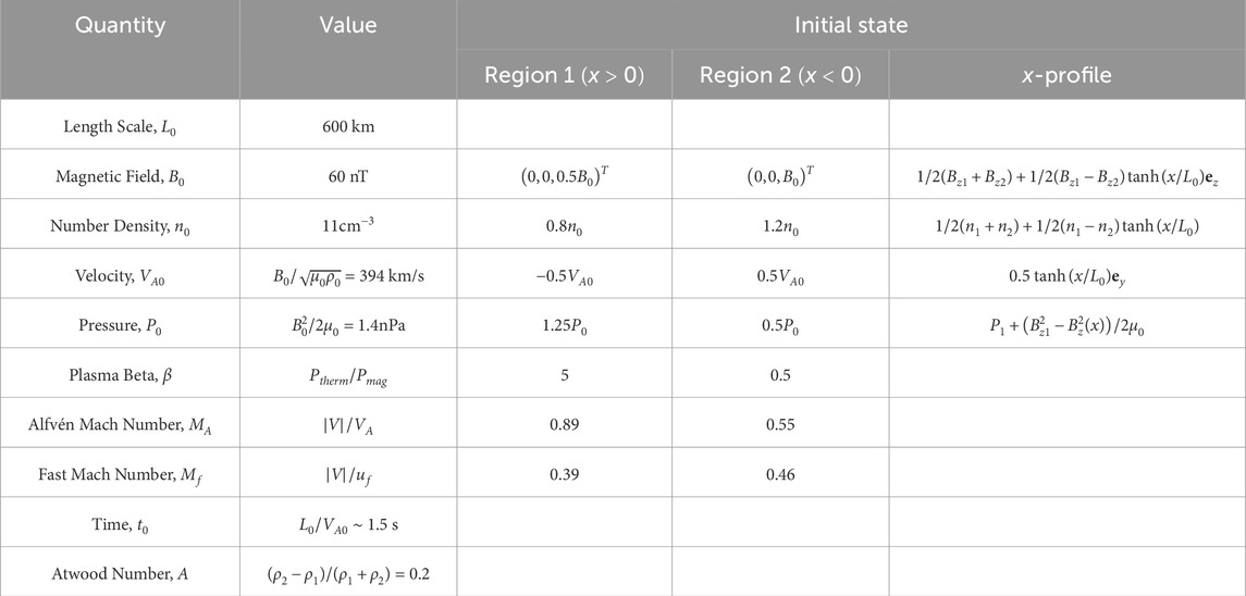
Table 1. Table showing the normalisation constants and initial state used in the simulation.

The whole simulation domain is given by $[-L_x,L_x]\times [-L_y,L_y]\times [-L_z,L_z]$ along the $x$-, $y$-, and $z$-directions, where $L_x=25L_0$, $L_y=10L_0$, and $L_z=120L_0$. The grid has 203 cells in each direction with a resolution of $0.1L_0$ in the $y$-direction, $0.6L_0$ in the $z$-direction and is stretched along the $x$-direction with a minimum resolution of $0.1L_0$. The boundary conditions along the $y$-direction are periodic. Along the $x$-direction, the boundaries are closed, in which $v_x=0$ and ${\partial }_x=0$ for the rest of the quantities. The dimension along $x$ is large enough to ignore the influence from the boundaries such as MHD wave reflections. To maintain the top boundary from the perturbation, an artificial friction term $-\nu (z)(\mathbf{v}-{\mathbf{v}}_{\mathbf{0}})$ is applied to the right-hand side of the momentum equation in the simulation (Ma et al., 2017). Here, ${\mathbf{v}}_{\mathbf{0}}$ is the unperturbed bulk velocity, which also represents the solar wind or ionosphere speed. The friction term tends to force the plasma to move at its initial velocity, or equivalently it absorbs perturbations, maintaining the initial boundary layer away from the equatorial plane. The friction coefficient is given by $\nu (z)=0.5\{2-\tanh [(z+z_{\nu })/L_0{D}_{\nu }]+\tanh [(z-z_{\nu })/L_0{D}_{\nu }]\}$, $z_{\nu }=30L_0$, and $D_{\nu }=3$, which has been switched on only near the top and bottom boundaries (Ma et al., 2017; Ma et al., 2021b).

To overcome issues with Fourier analysis and noise from differentiation, we trilinear interpolate all the data to a regular grid of resolution $0.1L_0$ in all directions for our investigations. The simulation boundary conditions are valid for the Fourier approach to the Helmholtz decomposition of the magnetic tension. The $y$-boundary is periodic, which a Fast Fourier Transform assumes. The $x$-dimension is suitably large that perturbations decay before reaching the simulation edges (the $x$-extent of the simulation is twice that shown in Figure 1). The large dimension along the $z$-direction, along with the frictional term at the boundary, means that the Alfvén wave is fully damped before it reaches the top/bottom simulation edges. We found no evidence of Gibbs effects present from the application of Fourier approach to the Helmholtz decomposition.

Figure 1

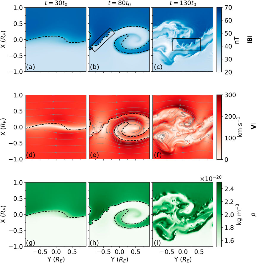
Figure 1. An equatorial $(z=0)$ view of the magnitude of the magnetic field, magnitude of the velocity, and density at the quasi-linear $(t=30t_0)$ (panels A,D,G), nonlinear surface roll-up $(t=80t_0)$ (panels B,E,H) and turbulent $(t=130t_0)$ stages (panels C,F,I) of the simulation. The black boxes in panels b and c highlight secondary KHI. The dashed black line is plotted along $\rho ={\rho }_0$ contour as a proxy for the boundary between the two sides. There are streamlines present in grey on the velocity plots to demonstrate the velocity shear.

The initial steady state is a one-dimensional transition layer with a flow shear, the conditions of which are outlined in Table 1. This transition layer is initially imposed by a hyperbolic tangent function with characteristic thickness of $L_0$ and maintains the total force balance across the sheared flow layer (i.e., the sum of the thermal pressure and magnetic pressure is constant). The KHI is triggered by a velocity perturbation localised in the vicinity of the equatorial plane (i.e., $z=0$), which is given by $\mathbf{v}=\nabla \mathrm{\Phi }(x,y)\times {\mathbf{e}}_{z}f(z)$. Here, the stream function is $\mathrm{\Phi }(x,y)=\delta v\cos (k_{y}y){\cosh }^{-2sec}(x/l_x)$, normal scale of the perturbation $l_x=2L_0$, KH wavenumber $k_y=\pi /L_y$, amplitude of the velocity perturbation $\delta v=V_{A0}/20$, and the localisation function $f(z)$ is given by $f(z)=0.5\{\tanh [(z+z_d)/L_0{D}_z]-\tanh [(z-z_d)/L_0{D}_z]\}$, where $z_d=20L_0$, and $D_z=3$.

Figure 1 shows 3 snapshots of the simulation in the equatorial plane. $t=30t_0$ is approximately during the quasi-linear surface wave stage, $t=80t_0$ is during the nonlinear surface roll-up stage of the KHI, and $t=130t_0$ is during the turbulent stage beyond the surface roll-up. These three stages are used throughout this work. At time $t=80t_0$, and $t=130t_0$ there are secondary KHI forming as highlighted in panels 1b and 1c. The dashed black line is plotted along the $\rho ={\rho }_0$ line as a visual aid to the reader for identifying the proxy-boundary. As $M_f\sim 0.4$ this proxy-boundary should be little affected by compressible effects. Note also that different methods of magnetopause identification in simulations are known not to always be co-located (García and Hughes, 2007; Gordeev et al., 2013). It does not feature in the turbulent stage as there is no clear boundary between the two sides.

4.2 Results and discussion

4.2.1 Exploring $P_{\mathrm{ten}}$

A key step in the derivation of ${\lambda }_{\text{MHD}}$ is the realisation that a part of the magnetic tension contributes to the pressure-like forces on the plasma, with this achieved through a Helmholtz decomposition of the magnetic tension into rotational and irrotational vector fields. Figure 2 shows this decomposition. In the quasi-linear stage $(t=30t_0)$, tension is shown to be acting as a stabilising force opposing the deformation of the boundary as expected. The tension is entirely rotational in this initial stage, as expected for a linear incompressible surface wave (Plaschke, 2016). This implies the tension field is not yet perturbed enough to provide a (nonlinear) pressure-like contribution. In the nonlinear surface roll-up stage $(t=80t_0)$, the tension field has become sufficiently twisted for the tension to start exhibiting a pressure-like part, but the tension overall is still predominantly rotational. The force is again pointing in directions to try and restore the boundary to its original shape–with the pressure-like part now also contributing to this. In the turbulent stage $(t=130t_0)$ it becomes unclear on the behaviour of the tension as the KHI-generated structures have evolved turbulently–it is however clear that the forces are still predominantly rotational. The tension generally has a larger magnitude in regions where secondary KHI are present.

Figure 2

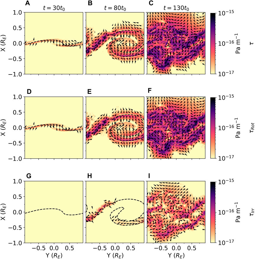
Figure 2. An equatorial $(z=0)$ view of the total $\mathit{\tau }$, irrotational part, ${\mathit{\tau }}_{\mathit{Irr}}$, and rotational part, ${\mathit{\tau }}_{\mathit{Rot}}$, of the magnetic tension as found through a Helmholtz decomposition. In colour is the magnitude with overlaying unit vectors to indicate the acting direction in the $xy$-plane. The quasi-linear $(t=30t_0)$ (panels A,D,G), nonlinear surface roll-up $(t=80t_0)$ (panels B,E,H), and turbulent $(t=130t_0)$ stages (panels C,F,I) of the simulation are shown. The dashed black line is plotted along $\rho ={\rho }_0$ contour as a proxy for the boundary between the two sides.

Since ${\lambda }_{\text{MHD}}$ relies upon finding an effective pressure minimum, we show the various forms of pressure in Figure 3. Here the variation of the pressure fields about their respective mean is shown–this eliminates any bias from $P_{\text{ten}}$ lacking uniqueness. In the quasi-linear stage, the effective pressure has a single minimum near the centre of the simulation between the points where the boundary is most deformed. In the nonlinear stage, the effective pressure has a minimum near the centre of the surface roll up. There is now also an obvious maximum adjacent to it. Along the boundary in the region of secondary KHI (as highlighted in Figure 1B) several small-scale effective pressure minima are also present. There are also other minima in regions where it is clear turbulence/inhomogeneity is present by looking at the other pressures. It is evident that $\delta P_{\text{Ten}}$ does not play a major role in how the total effective pressure is defined as it is generally an order of magnitude smaller than the other pressure variations. $\delta P_{\text{Ten}}$ becomes larger in regions where the magnetic field lines are contorting, but overall it is smaller than $\delta P_{\text{therm}}+\delta P_{\text{mag}}$. This can also be seen in Figure 3C where the $\delta P_{\mathit{Ten}}$ minima appear to sit along the upper and lower boundaries of the mixed/turbulent plasma and the homogeneous plasma.

Figure 3

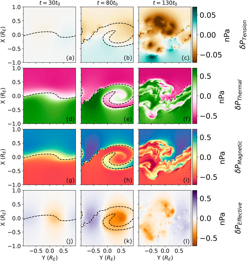
Figure 3. An equatorial $(z=0)$ view of the perturbations from the mean pressure due to magnetic tension, thermal pressure, magnetic pressure, and total pressure. The quasi-linear $(t=30t_0)$ (panels A,D,G,J), nonlinear surface roll-up $(t=80t_0)$ (panels B,E,H,K) and turbulent $(t=130t_0)$ stages (panels C,F,I,L) of the simulation. The dashed black line is plotted along $\rho ={\rho }_0$ contour as a proxy for the boundary between the two sides.

Like the tension force itself, $\left|\delta P_{\text{Ten}}\right|$ appears to be largest in regions where secondary smaller-scale KHI structures are present. This is likely down to the following two reasons. Firstly, recall that magnetic tension is related to the curvature of field lines, meaning rolled-up smaller scale structures will have greater tension. Additionally, the growth rate of smaller scale structures is greater than larger scale ones (Nagano, 1979; Sundberg et al., 2010; Rice et al., 2022) meaning they will roll-up and evolve faster, i.e., increasing the field line curvature.

4.2.2 Validating ${\lambda }_{\mathrm{MHD}}$

Section 4.2.1 demonstrates that the contributions to the effective pressure from the pressure-like part of the magnetic tension are small for this simulation. Consequently, hydrodynamic techniques might be sufficient in identifying vortices for the simplified magnetopause in this simulation. We therefore compare ${\lambda }_{\text{MHD}}$ to the other vortex criteria mentioned in Section 2.2.

The different vortex methods are applied to every cell in the simulation, where spatial derivatives are undertaken through second order accurate central differences in the interior points and first order accurate differences at the boundaries. To remove machine noise in the gradients we apply a multidimensional Gaussian filter with a standard deviation of 0.5 grid cells. The smoothed data is then passed through a $3\times 3\times 3$-cell multidimensional median filter to ensure that the regions are ‘connected’ – meaning that more than one adjacent cell in a plane must be identified as vortical for a positive identification. Typically with these types of techniques a threshold is chosen to define a vortex (Dong and Tian, 2020), however we have chosen not to do this to allow for a more complete comparison of the techniques and what they physically represent.

Figure 4 shows the ${\lambda }_{\text{MHD}}$ vortex definition compared to the 2-dimensional velocity streamlines ($v_z$ is negligible throughout this plane) to qualitatively assess whether the technique is correctly identifying vortices. In the quasi-linear stage of the KHI $(t=30t_0)$, there is a single vortex core identified (region 1) which is centred around the steep edge of the deformed shear flow boundary. After some evolution to the nonlinear roll-up stage $(t=80t_0)$, the previous vortex has now evolved and been stretched and torn into four large structures (regions 2, 4, 5, 6). The strongest signature in the simulation is region 2, a structure at the edge of the simulation that is the leading edge of the rolled up surface (remembering the boundary conditions in $y$ are periodic). The other three structures are in the centre of the simulation, again where the surface roll-up is present. Interestingly, the secondary small-scale KHI vortices (region 3) have a stronger signature than the three vortex structures within the roll-up (regions 4, 5, 6). It appears the vortices are all situated where the principal curvature of the boundary is greatest, with the strength being proportional in some way to the curvature of the boundary i.e., stronger vortices deform the boundary more.

Figure 4

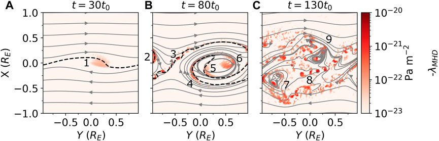
Figure 4. An equatorial $(z=0)$ view of vortex identification method $-{\lambda }_{\text{MHD}}$ values on a ${\text{log}}_{10}$ colour-scale. The quasi-linear $(t=30t_0)$ (panel A), nonlinear surface roll-up $(t=80t_0)$ (panel B) and turbulent $(t=130t_0)$ stages (panel C) of the simulation. In grey are 2D velocity field streamlines. The numbers in the plot indicate regions of interest discussed in the text. The dashed black line is plotted along $\rho ={\rho }_0$ contour as a proxy for the boundary between the two sides.

The original large-scale vortex becomes unidentifiable in the turbulent stage, it is possible that region 4 becomes region 7 and region 5 becomes region 9, but this is ambiguous. Instead strong ${\lambda }_{\text{MHD}}$ signatures are present in much of the simulation domain due to lots of small-scale vortical structures being present throughout. There are two large vortices present (regions 7 and 9). Some of the strongest signatures are found where secondary KHI is present (region 8). Generally, speaking ${\lambda }_{\text{MHD}}$ grows with time as the strongest signatures are seen in the turbulent stage and the weakest in the quasi-linear stage.

Figure 5A shows a zoom in of vortex region 4 from the nonlinear roll-up stage. In the simulation frame the vortex is not immediately apparent in the flow, despite ${\lambda }_{\text{MHD}}$ identifying a distinct vortex in this region. However, exploiting the Galilean invariance of the method, we transform the velocity field into a different frame in panel b. This clearly demonstrates an isolated vortex is present, hence the distinct regions identified by ${\lambda }_{\text{MHD}}$ within the KHI roll-up are real vortical features in the flow. This again highlights the need for vortex identification techniques, since they can pinpoint vortices which are not clear from visual analysis. We emphasise that the vortices these techniques identify are not simply the large-scale roll-up structure of the boundary overall, but flow vortices present as substructure within this roll-up which are ultimately responsible for the boundary deformations.

Figure 5

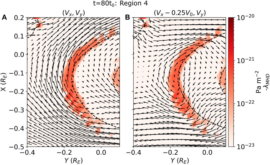
Figure 5. An equatorial $(z=0)$ view of vortex identification method $-{\lambda }_{\text{MHD}}$ values on a ${\text{log}}_{10}$ colour-scale. Region 4 (see Figure 4B) of the nonlinear surface roll-up $(t=80t_0)$ stage is shown. Panel a and b show the same ${\lambda }_{\text{MHD}}$ colour map calculated in the simulation frame. In black are 2D velocity field quivers, panel (A) shows the original velocity field quivers, panel (B) shows a Galilean transformed field where the $V_x^{\prime }=V_x-0.25V_{A0}$. The dashed black line is plotted along $\rho ={\rho }_0$ contour as a proxy for the boundary between the two sides.

Figure 6 shows the MHD effective pressure with overlaying contours of the different vortex identification methods (${\lambda }_{\text{MHD}}$ and those mentioned in Section 2.2), which should identify pressure minima. Contour levels have been arbitrarily chosen to display behaviour at extremes of large and small values that constitute a vortex (without any data-driven thresholds imposed; cf. Dong and Tian, 2020) for more comprehensive comparison of the different methods. Visually comparing the hydrodynamic criteria and ${\lambda }_{\text{MHD}}$, it appears that all the definitions of a vortex identify similarly compact regions. This further qualitatively validates ${\lambda }_{\text{MHD}}$ and also suggests the simpler hydrodynamic criteria may be used as proxies for ${\lambda }_{\text{MHD}}$. Since each method makes different levels of assumptions about the fluid, comparing the different definitions explores how introducing these different physical effects affects the regions identified as a vortex core, hence their importance in vortex formation and evolution.

Figure 6

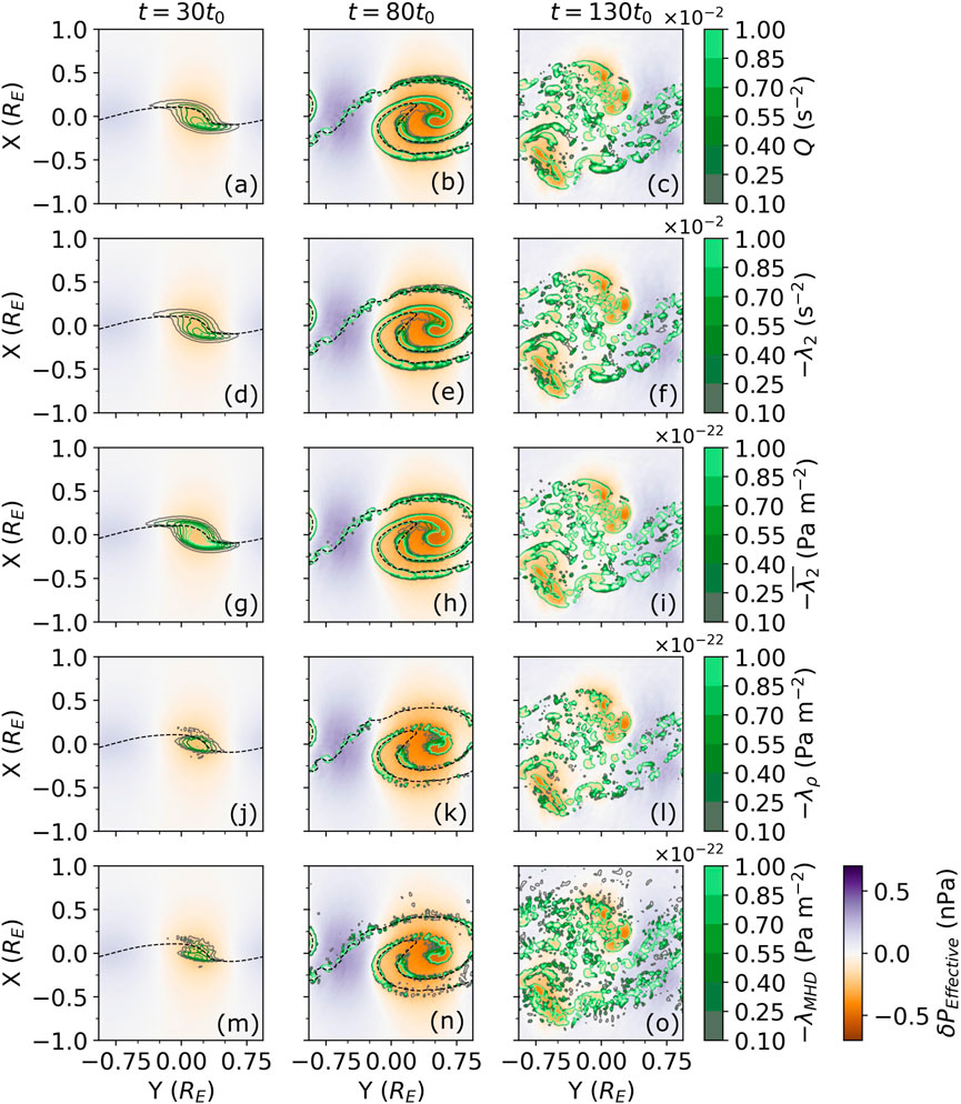
Figure 6. An equatorial $(z=0)$ view of contours for different vortex techniques on a linear colour-scale. These are plotted over the effective pressure variations from the mean. The quasi-linear $(t=30t_0)$ (panels A,D,G,J,M), nonlinear surface roll-up $(t=80t_0)$ (panels B,E,H,K,N), and turbulent $(t=130t_0)$ stages (panels C,F,I,L,O) of the simulation. The dashed black line is plotted along $\rho ={\rho }_0$ contour as a proxy for the boundary between the two sides.

$Q$ and ${\lambda }_2$ perform almost identically across the three time steps shown in Figure 6 and identify similar regions to those discussed in Figure 4. The criteria identify regions where the local boundary is most deformed and by comparing to effective pressure in Figure 3, it is clear that they are locating local pressure minima in the quasi-linear stage. In the nonlinear and turbulent stages, this is less clear. The minima located by them differ to the local minima in the effective pressure plots. The effective pressure appears to highlight the general region however the criteria clearly outlines the vortex core regions. This is because the neglected parts of the adapted effective pressure Hessian are non-negligible in these stages and neglecting them allows for a clearer identification. This suggests that making these adaptations to the pressure Hessian are vital to the success of the $\lambda$-family of techniques. Furthermore, it demonstrates that while local total pressure minima may be reliable in the quasi-linear stage as an approximate identification tool, beyond this the method is not precise enough and advanced vortex identification techniques are necessary.

Comparing $Q$ and ${\lambda }_2$ to $\overline{{\lambda }_2}$ probes the importance of momentum flow over velocity flow in the identification of a vortex. Crucially, the power and strength of those regions shift to locations where there is larger vortical momentum instead of just vortical velocity. Since $\overline{{\lambda }_2}$ simply weights ${\lambda }_2$ by local density, the sign remains unchanged and thus it identifies identical regions to ${\lambda }_2$. Unlike $Q$ and ${\lambda }_2$, the units of $\overline{{\lambda }_2}$ are comparable to those of ${\lambda }_{\text{MHD}}$ allowing for direct comparisons to be made between the two criteria. In this simulation, the ${\lambda }_2$ and $\overline{{\lambda }_2}$ results do not appear to differ much–this is likely due to the uniform initial density along the shear direction. Comparing the results of ${\lambda }_{\rho }$ to that of $\overline{{\lambda }_2}$ allows for an insight into how fluid compressibility and density gradients influence where a vortex core is identified. It is apparent that these two factors do influence vortex identification as there is an obvious reduction in the volume that ${\lambda }_{\rho }$ identifies as vortical compared to the less advanced methods. In particular, the vortex appears less strongly in ${\lambda }_{\rho }$ at the $t=30t_0$ stage compared to the earlier considered methods. In the later stages of the KHI, there are more detached vortical regions seen in ${\lambda }_{\rho }$ compared to the less advanced methods. This suggest that ${\lambda }_{\rho }$ is capable of distinguishing between multiple vortices in close proximity. The less advanced methods appear to smear these multiple vortices into one large vortex core structure making them less useful if studying vortex shedding, complex regions, or turbulent stages. Due to this, ${\lambda }_{\rho }$ is better suited for revealing finer details of the complex physics taking place.

${\lambda }_{\text{MHD}}$ includes the influence of the magnetic field to the definition of a vortex core. ${\lambda }_{\text{MHD}}$ appears to identify almost the same structures as ${\lambda }_{\rho }$, indicating that magnetic tension may not play a dominant role in the large-scale vortices in this simulation. This is somewhat expected since under northward IMF the magnetic tension is least effective at suppressing the KHI, and the scale of variations along the anchored field lines are much larger than those perpendicular to the field (Equation 1). Nonetheless, ${\lambda }_{\text{MHD}}$ does identify additional finer-scale archipelago-like structures less dominant in the hydrodynamic approaches. These occur at the small-scale secondary KH vortices, likely because the tension term becomes more important in these regions as previously discussed in Section 4.2.1. As many of these values are relatively close to zero, this may suggest that in practical applications a higher threshold value than the lowest contour displayed of $0.01\times 10^{-22}$ Pa ${\mathrm{m}}^{-2}$ may be needed for the ${\lambda }_{\text{MHD}}$ (and maybe ${\lambda }_{\rho }$) technique(s). This would reduce the number of small scale structures being identified, enabling focus on stronger vortices and their large-scale structure. How best to set such vortex thresholds is an area of ongoing research even in hydrodynamics (Chakraborty et al., 2005; Pierce et al., 2013; Liu et al., 2019; Dong and Tian, 2020).

Figure 7 shows 2-dimensional histograms over the entire simulation domain quantitatively comparing each hydrodynamic vortex criterion (vertical axes) with ${\lambda }_{\text{MHD}}$ (horizontal axes). In all the histograms there is a main data population confined to a $y\propto x$ line (except for Q where the criteria for a vortex is positive not negative making it $y\propto -x$ instead) meaning all the techniques have a good correlation with ${\lambda }_{\text{MHD}}$ – especially ${\lambda }_{\rho }$ during the linear and nonlinear stages. This is reflected in the strong Pearson’s correlation coefficients, $R$. There are two secondary populations in the histograms. The first is along the $y=0$ region–largely with negative ${\lambda }_{\text{MHD}}$ values. These correspond to regions where ${\lambda }_{\text{MHD}}$ has identified a vortex where the hydrodynamic definition has not. Assuming ${\lambda }_{\text{MHD}}$ is successfully identifying vortices and given the only difference between it and the ${\lambda }_{\rho }$ definition is the introduction of the rotational tension term, this feature must be due to magnetic field effects that ${\lambda }_{\text{MHD}}$ is able to extract which the hydrodynamic definitions cannot. The second is around the $x=0$ region, this is due to the hydrodynamic definitions identifying larger regions as vortical compared to ${\lambda }_{\text{MHD}}$. This supports the previous finding that the simpler hydrodynamic definitions have a poorer precision than ${\lambda }_{\rho }$ or ${\lambda }_{\text{MHD}}$. As the simulation becomes turbulent, there is a larger variance about the linear relationship between the hydrodynamic and MHD methods, though the correlation is still reasonable. The increased variance is expected as, e.g., the magnetic tension term becomes more important in the small-scale structures which form. An analysis of each technique’s performance against ${\lambda }_{\text{MHD}}$ can provide a better understanding of how different regimes can affect vortex formation and identification.

Figure 7

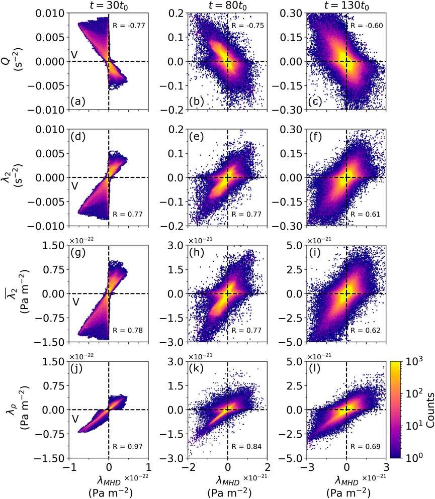
Figure 7. 2D histograms across the entire simulation domain comparing ${\lambda }_{\text{MHD}}$ with the hydrodynamic vortex criteria. Counts are plotted using a ${\text{log}}_{10}$ colour scale. The quadrant which represents a vortex in both ${\lambda }_{\text{MHD}}$ and the comparison definition is labelled with ‘V’. The $R$ value denotes Pearson’s correlation coefficient. Analysis of the quasi-linear (t = 30t₀) (panels A,D,G,J), nonlinear surface roll-up (t = 80t₀) (panels B,E,H,K), and turbulent (t = 130t₀) stages (panels C,F,I,L) are shown.

The $Q$, ${\lambda }_2$, and $\overline{{\lambda }_2}$ comparisons all demonstrate good correlations with the ${\lambda }_{\text{MHD}}$ technique which strongly suggests that compressibility and plasma inhomogeneity do not play a significant role in the identification of the vortex, as these techniques are ignorant of these effects. The secondary populations break this pattern and are not as present in ${\lambda }_{\rho }$ which reinforces that the regions identified by the simplest hydrodynamic criteria are not as precise as the more advanced methods. Previous research has found that the simpler hydrodynamic techniques struggle to distinguish between two vortices situated close together in space and tend to blur the volumes into one large structure (Cai et al., 2018; Collado-Vega et al., 2018) – our results agree with these findings.

The square of Pearson’s correlation coefficient between ${\lambda }_{\rho }$ and ${\lambda }_{\text{MHD}}$ indicates the amount of variance in ${\lambda }_{\text{MHD}}$ explainable by hydrodynamic effects alone. ${\lambda }_{\rho }$ has a very good Pearson’s correlation coefficient with ${\lambda }_{\text{MHD}}$ of 0.97 in the quasi-linear stage, hence vortex identification is virtually entirely described by hydrodynamics and magnetic effects are negligible during this early stage of the KHI within this simulation (again likely due to the northward IMF conditions used along with long field lines). As it evolves into the nonlinear surface roll-up stage, hydrodynamics only explains $71\%$ of the variations present. Magnetic tension term therefore plays a non-negligible role, likely due to magnetic tension’s effects becoming more important as secondary KHI begin to form. In the turbulent stage of the KHI, less than half $\left(47\%\right)$ of the variations in ${\lambda }_{\text{MHD}}$ are due to hydrodynamic effects alone, meaning that magnetic tension becomes an essential component likely due to the increased number of smaller-scale magnetic structures present.

The analysis has shown that (for this simulation at least) $Q$, ${\lambda }_2$, and $\overline{{\lambda }_2}$ are good approximations of a vortex in the MHD regime. However, they are prone to false-identifications as they struggle to distinguish between multiple vortices in close proximity. Including density gradient and compressibility effects allows ${\lambda }_{\rho }$ to more successfully distinguish between these close proximity vortices, allowing it to provide more precise vortex identifications. Effects from magnetic tension, only incorporated into ${\lambda }_{\text{MHD}}$, become more important over time due to structural evolution and field line twisting, wrapping, and distortion. While the different vortex criteria include and/or exclude different physical effects related to vortex formation, quantitatively comparing these eigenvalues does not self-consistently enable a thorough investigation of the interplay these physical effects since each criterion has a different eigenvector. A different quantitative method needs to be used to fully explore how each different term, and therefore effect, influences vortex identification.

4.2.3 Contributions to ${\lambda }_{\mathrm{MHD}}$

As derived in Section 3.2, there are four physical effects which contribute to ${\lambda }_{\text{MHD}}$: vortical momentum $\left(\mathbf{M}\right)$, fluid compressibility $\left(\mathbf{C}\right)$, density gradients $\left(\mathbf{D}\right)$, and the rotational tension $\left(\mathbf{T}\right)$. Here we investigate to what extent each contributes to ${\lambda }_{\text{MHD}}$ within the simulation.

The effective pressure Hessian tensor, $\mathbf{H}$, is real and symmetric (hence also Hermitian). It therefore has real eigenvalues whose eigenvectors can be chosen to be real and orthonormal. From the spectral theorem the Hessian’s eigenvalue can be rewritten as a linear combination of eigenvector projections, known as a spectral eigendecomposition. Let ${\widehat{\mathbf{V}}}_{H,2}$ be the normalised eigenvector of $\mathbf{H}$ corresponding to the second eigenvalue, ${\lambda }_{\text{MHD}}$. Right multiply Equation (23) by ${\widehat{\mathbf{V}}}_{H,2}$ and left multiply by the transpose to get,

${\lambda }_{\text{MHD}}=-{\widehat{\mathbf{V}}}_{H,2}^T\mathbf{H}{\widehat{\mathbf{V}}}_{H,2}(\mathrm{24a})$

$={\widehat{\mathbf{V}}}_{H,2}^T\mathbf{M}{\widehat{\mathbf{V}}}_{H,2}+{\widehat{\mathbf{V}}}_{H,2}^T\mathbf{D}{\widehat{\mathbf{V}}}_{H,2}+{\widehat{\mathbf{V}}}_{H,2}^T\mathbf{C}{\widehat{\mathbf{V}}}_{H,2}+{\widehat{\mathbf{V}}}_{H,2}^T\mathbf{T}{\widehat{\mathbf{V}}}_{H,2}(\mathrm{24b})$

$={\lambda }_M+{\lambda }_D+{\lambda }_C+{\lambda }_T.(\mathrm{24c})$

For clarity ${\lambda }_{M,D,C,T}$ are not eigenvalues of their respective matrices, but are the contributions to the ${\lambda }_{\text{MHD}}$ eigenvalue of $\mathbf{H}$. This demonstrates how each term directly contributes to ${\lambda }_{\text{MHD}}$ which allows for quantitative analysis and comparison of the different contributions each physical effect has on ${\lambda }_{\text{MHD}}$. It is widely accepted that magnetic tension is a stabilising force for the KHI so it is sensible the derivation has it subtracted instead of added. Regions where tension acts to stabilise, i.e., regions where a vortex exists, thus become identified as vortical.

Figure 8 shows a spatial map of the contribution each term has to ${\lambda }_{\text{MHD}}$ at each of the three stages considered. The values shown are processed like before. In overview, it is clear that the vortical momentum term (panels a–c) generally dominates the ${\lambda }_{\text{MHD}}$ definition, supporting the conclusion that $Q$, ${\lambda }_2$, and $\overline{{\lambda }_2}$ are reasonable approximations of ${\lambda }_{\text{MHD}}$. The other terms appear to act as corrections to the vortical momentum term. Density gradients (panels d–f) generally oppose the vortical momentum. The fluid compressibility term (panels g–i) is generally small at all three stages shown. Over the course of the three stages, the rotational component of the magnetic tension (panels j–l) tends to grow in regions where smaller-scale vortices form, reinforcing its importance over these scales. However, all the terms appear to have a complex relationship with ${\lambda }_{\text{MHD}}$ overall, supporting in some locations but opposing in others.

Figure 8

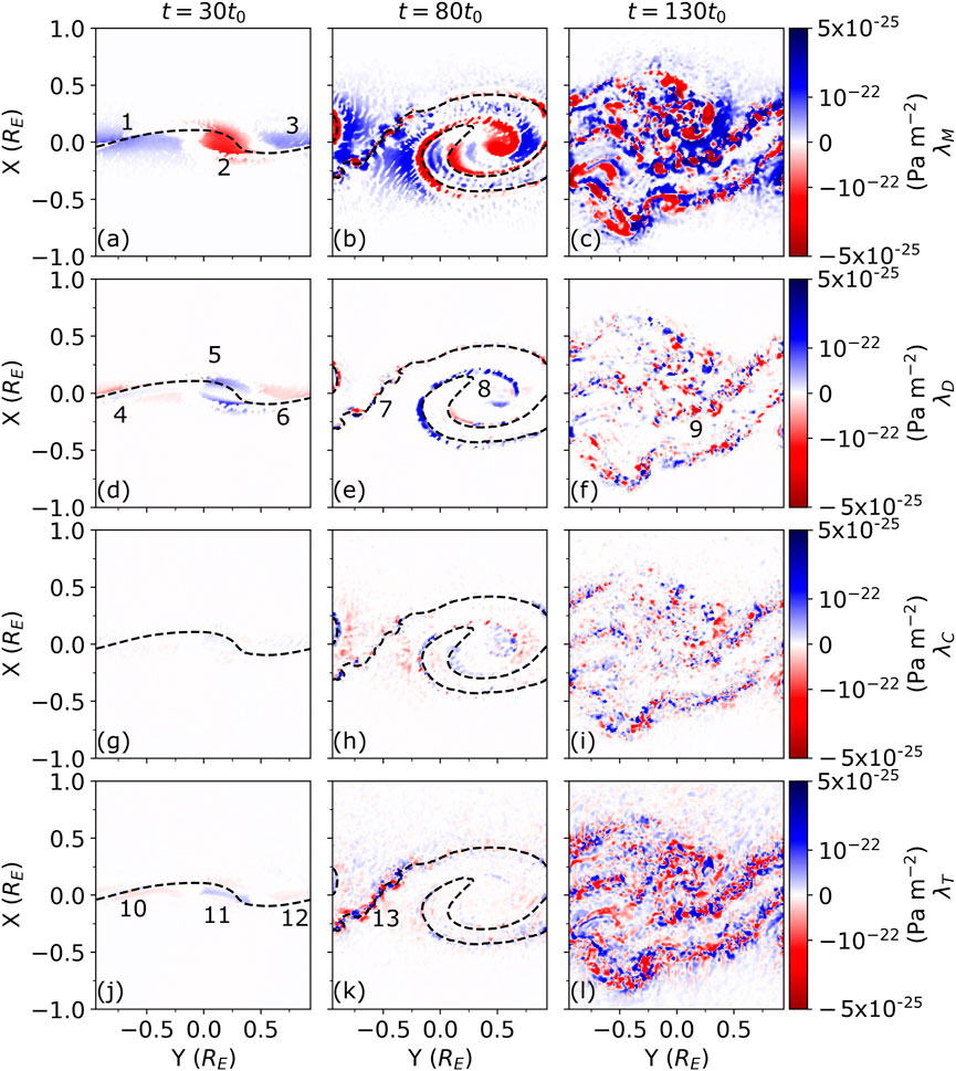
Figure 8. An equatorial $(z=0)$ view of each contributing term to ${\lambda }_{\text{MHD}}$. The values on a ${\text{symlog}}_{10}$ colour-scale where the linear scale is between $\pm 10^{-22}$ Pa ${\mathrm{m}}^{-2}$. Negative regions (red) support ${\lambda }_{\text{MHD}}$, positive values (blue) are regions in opposition with ${\lambda }_{\text{MHD}}$. The quasi-linear $(t=30t_0)$ (panels A,D,G,J), nonlinear surface roll-up $(t=80t_0)$ (panels B,E,H,K) and turbulent $(t=130t_0)$ stages (panels C,F,I,L) are shown. The dashed black line is plotted along $\rho ={\rho }_0$ contour as a proxy for the boundary between the two sides.

In the quasi-linear stage, vortical momentum is the dominant term. There are two different populations in this term, the first (region 2) is in support of a vortex and lies between where the interface is most deformed. The other population (regions 1 and 3) oppose a vortex. Density gradients (panel d) oppose the formation of a vortex at the centre of simulation (region 5). Interestingly, this opposition is strongest at the edges along the normal of the vortical momentum region (2) rather than at the centre. This serves to reduce the volume being identified as vortical and is the reason the ${\lambda }_{\text{MHD}}$ method is more precise, allowing for better vortex core identification. This suggests that the density gradient term is crucial for the reliable identification of multiple vortices in close proximity. Furthermore, the density gradient term contributes to the existence of vortices at the outer edges of the simulation near the boundary (regions 4 and 6) where vortical momentum is not present (regions 1 and 3) – this may alternatively be a reduction in the non-vortex signature provided by the momentum term. Further investigation is needed into the physical interpretation of this, which we leave to future work since overall these regions are not identified as vortices. Compressibility appears negligible at this stage. The rotational tension term is complex in regions 10, 11, 12 – there is weak opposition along the boundary (the dashed line) in regions 10, 11, and 12 implying tension is acting to stabilise the boundary as expected. However, the term appears to weakly support off the boundary in these regions too. Reasoning for this is unclear. It is worth noting that regions 4 and regions 10 look very similar, as do regions 6 and 12 however this may just be a consequence of the structure shape.

In the nonlinear surface roll-up stage, the density gradient term strongly opposes the larger scale vortex (region 8) but has little power on the small-scale secondary KHI (region 7) implying the term may have a scale–or KHI-stage–bias. The density gradient term appears to have the same relationship with the small-scale secondary KH vortices (region 7) as it has with the single vortex in the quasi-linear stage–it opposes the formation of a vortex at the centre of simulation on edges of the region of vortical momentum, but not at the centre where it supports it. The compressibility term does not appear to show any obvious trend and is generally small at this stage. The rotational magnetic tension term has become large in region 13 where the small-scale secondary KH vortices are present, opposing their formation. It appears to have little impact on the large scale vortex.

In the turbulent stage, the density gradient term appears to have the same relationship with the small-scale secondary KH vortices (region 9) as it has with the single vortex in the quasi-linear stage. This was also seen in region 7 meaning that the relationships between the physical effects for the secondary KHI at these stages can be considered as analogous to those for the large-scale vortex during its quasi-linear stage. The compressibility term again remains small with no clear relationship to the vortices. Rotational magnetic tension has further grown, now opposing the secondary KH vortices.

These trends have only been qualitatively explored in the equatorial plane. Further quantitative analysis can be made to better understand the general contributions over the entire simulation domain.

Figure 9 shows 2-dimensional histograms of the entire simulation domain comparing each term in Equation 24c with ${\lambda }_{\text{MHD}}$. Across all three time steps the fluid compressibility term is small and poorly correlated to ${\lambda }_{\text{MHD}}$ implying that fluid compressibility is not a dominant component in the existence of a KH vortex in this simulation. This might be attributed to the low convective fast magnetosonic Mach number used in this simulation, meaning the plasma is weakly compressible (representative of the near-flank magnetopause environment; Ma et al., 2020).

Figure 9

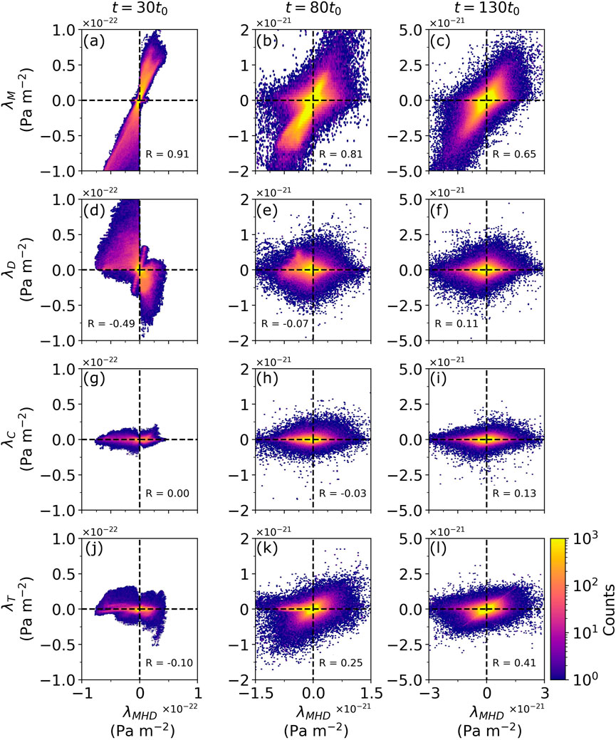
Figure 9. A 2D histogram across the simulation domain comparing ${\lambda }_{\text{MHD}}$ with the terms contributing to it. Counts are plotted using a ${\text{log}}_{10}$ colour scale. The R value shown is the Pearson’s correlation coefficient. Analysis of the quasi-linear (t = 30t₀) (panels A,D,G,J), nonlinear surface roll-up (t = 80t₀) (panels B,E,H,K), and turbulent (t = 130t₀) stages (panels C,F,I,L) are shown.

Figure 9D shows that the density gradient term strongly opposes the formation of a vortex in the quasi-linear stage of its growth but becomes less significant in the later stages. This suggests that the density difference across the shearing fluid is important in the initial stages of KH wave formation. Physically this makes sense, as the flow with a lower density will have insufficient momentum to change the direction of the high momentum flow with heavier mass making the initial wave harder to generate. Beyond the quasi-linear stage, the flow is sufficiently deformed that this density variation becomes less significant in comparison to the driving shear flow. There is a smaller secondary population in this term which supports the vortex and can also be seen in Figure 8D.

Figures 9J–L also indicates that the rotational component of the magnetic tension term becomes larger as the KHI advances. The plot suggests that during the turbulent stage, where vortices are expected to have a small spatial volume and thus larger tension effects, this term becomes a significant contributor to ${\lambda }_{\text{MHD}}$. This is also reflected in the Pearson’s correlation value. Finally, the rotational component of the magnetic tension term has multiple populations within itself. In the nonlinear stage, there is a population which sits along a $y\propto x$ line which will be the population where the term supports the identification of a vortex–this likely corresponds to the small scale secondary KH vortices. The second population sits along the $y=0$ line where the tension term does not contribute to ${\lambda }_{\text{MHD}}$ – this likely corresponds to the single large scale vortex. This pattern is also present in the turbulent stage. There is a strong population along a $y\propto x$ line indicating that this term is important in the turbulent stage. However, there is a larger spread in the $y=0$ population which may be because the histograms include the entire simulation domain and so will contain variations out-of-plane which are not seen in Figure 9.

4.2.4 Potential in situ applications

So far ${\lambda }_{\text{MHD}}$ has been applied to gridded simulation data. However, it would be helpful to also explore its potential application to multi-point in situ measurements, though somewhat challenging. While the momentum and density gradient terms involve only first-order spatial derivatives, thus can be calculated with four suitably instrumented spacecraft in a tetrahedron, e.g., Magnetospheric Multiscale (MMS) (Burch et al., 2016), the compressibility term involves second-order derivatives which require 10 spacecraft that do not lie on any quadric surface (Zhou and Shen, 2024). Finally, the rotational tension term is challenging since it involves a Helmholtz decomposition, which is inherently non-local requiring information throughout space. It may be possible through Equation 8b and suitable interpolation methods to estimate the decomposition for a multi-spacecraft mission such as HelioSwarm (Klein et al., 2023). Determining how to do this, however, is beyond the scope of this study.

Given these limitations, we simply consider a tetrahedral spacecraft configuration and only use the momentum and density gradient terms to construct the adapted pressure Hessian–essentially an incompressible version of ${\lambda }_{\rho }$ denoted as ${\lambda }_{\rho }^{*}$ herein. Section 4.2.2 demonstrated ${\lambda }_{\rho }$ accurately approximates ${\lambda }_{\text{MHD}}$ in this simulation during the linear and nonlinear roll-up stages, with Section 4.2.3 showing compressibility and magnetic tensions make negligible contributions. We show an example application in Figure 10, which uses a spatial slice of the simulation data along the $y$-axis to emulate a spacecraft encounter with the magnetopause. The figure compares ${\lambda }_{\text{MHD}}$ with ${\lambda }_{\rho }$ and ${\lambda }_{\rho }^{*}$, demonstrating that ${\lambda }_{\rho }$ and ${\lambda }_{\rho }^{*}$ are near identical techniques which both approximate ${\lambda }_{\text{MHD}}$ well in the linear, and nonlinear stages here. Unsurprisingly, the techniques appear to be less useful in the turbulent stage, however, they do still replicate the ${\lambda }_{\text{MHD}}$ results overall. Thus ${\lambda }_{\rho }^{*}$ may be a sensible proxy which could be realised by tetrahedral in-situ data. The qualitative visual differences between the three stages suggests they may also be used to distinguish between different evolutionary phases; a prospect we leave for quantitative exploration in future work.

Figure 10

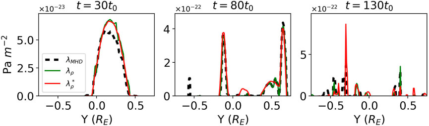
Figure 10. A spatial slice through the $x=z=0$ line of the simulation showing $-{\lambda }_{\text{MHD}}$, $-{\lambda }_{\rho }$, and $-{\lambda }_{\rho }^{*}$ values. Only the vortex identifying values are shown.

Regular tetrahedra of spacecraft are considered, with mesocentres along the $x$-axis. Simulation data are trilinearly interpolated to spacecraft locations. Since spacecraft separation affects the quality and scales over which gradients can be estimated (De Keyser, 2008), we vary the tetrahedra’s radial distances $r$ as 60 km, 100 km, and 200 km (the simulation grid spacing is 60 km). These cover the range of MMS separations over the course of the mission, excluding its smallest tetrahedron sizes. Gradients are calculated using techniques outlined in Paschmann and Daly (1998) and are used to calculate $Q$, ${\lambda }_2$, $\overline{{\lambda }_2}$, and ${\lambda }_{\rho }^{*}$. Figure 11 shows how each technique performs with different tetrahedra sizes, compared also with the true values from the simulation grid.

Figure 11

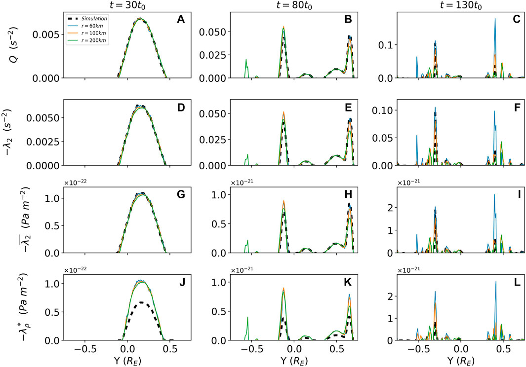
Figure 11. Vortex criteria values are shown using multi-spacecraft techniques with a mesocentre along the spatial slice through $x=z=0$ of the simulation with varying radial distances between spacecraft. Only the vortex identifying values are shown. Analysis of the quasi-linear (t = 30t₀) (panels A,D,G,J), nonlinear surface roll-up (t = 80t₀) (panels B,E,H,K), and turbulent (t = 130t₀) stages (panels C,F,I,L) are shown.

Figure 11 shows that all the techniques considered might be applied to virtual spacecraft observations with varying success. Generally speaking, the smaller the tetrahedron, the closer the virtual spacecraft value is to the simulation value. All the techniques reliably approximate the simulation values during the linear and nonlinear stages of the KHI regardless of virtual spacecraft separation. Interestingly, the smaller tetrahedron separation more precisely mimics the simulation results of all the techniques but contains larger amounts of noise, likely due to the interpolation–this is best seen in the quasi-linear stage. Notably, the widths of the peaks in the ${\lambda }_{\rho }^{*}$ technique are narrower than those in the less advanced techniques implying that a more specific region is being located by this technique–the core of the vortex. This is easiest seen when comparing Figures 11A,J.

5 Conclusion

The Kelvin-Helmholtz instability is a dominant driver of the viscous-like transfer of mass, momentum, and energy across the magnetopause through surface waves and their coupled vortices. A vortex detection method suitable for MHD, called ${\lambda }_{\text{MHD}}$, has been derived by self-consistently incorporating the $\mathbf{J}\times \mathbf{B}$ Lorentz force into the $\lambda$-family of hydrodynamic vortex identification techniques. These methods define a vortex as a local minimum within some 2D plane of an adapted pressure field. Within ideal MHD, the effective pressure field is defined as the sum of the thermal pressure, magnetic pressure, and the pressure-like part of the magnetic tension which is extracted using a Helmholtz decomposition. This is then adapted by removing the effects of unsteady straining, which can result in pressure minima unrelated to vortices, which is key to the $\lambda$-family methods’ success. ${\lambda }_{\text{MHD}}$ has been validated against the velocity field and other hydrodynamic techniques using a local three-dimensional MHD simulation representative of near-flank magnetopause conditions under northward IMF.

${\lambda }_{\text{MHD}}$ is composed of four components: vortical momentum, density gradients, fluid compressibility, and the rotational part of the magnetic tension. These effects have separately been shown to influence KHI formation (e.g., Chandrasekhar, 1961; Miura and Pritchett, 1982; Pu and Kivelson, 1983; Amerstorfer et al., 2010; Ma et al., 2024). In this work it was found that the vortical momentum dominates ${\lambda }_{\text{MHD}}$ in the simulation at all times, meaning that hydrodynamic techniques which capture this effect only, may be good proxies for ${\lambda }_{\text{MHD}}$. During the linear growth phase, density gradients generally act to oppose vortex formation but become less important in the later stages of vortex evolution. This is in agreement with previous work where plasma inhomogeneity was found to not affect growth rate (Ma et al., 2024). The rotational part of the magnetic tension has been shown to become important in small-scale structures suggesting that the hydrodynamic definitions would be insufficient at identifying these. Fluid compressibility was found to be insignificant at all stages.

Some of these results will be due to the choice of plasma parameters used, which are representative of the near-flank magnetopause. Dimensionless scaling arguments might infer the implications of this work under different plasma regimes though. The simulation is only weakly compressible $(M_f\sim 0.4)$, but compressibility effects are expected to vary as $\sim M_f^2$ (Palermo et al., 2011). Here we shall assume this scaling for the compressibility term, ${\lambda }_C$, and that the vortical momentum term, ${\lambda }_M$, might be unaffected by the convective Mach number. Over the three stages of the simulation presented, the ratio of these terms’ standard deviations, $\sigma ({\lambda }_C)/\sigma ({\lambda }_M)$, constitute $6\%$, $14\%$, and $21\%$ respectively. For the compressibility term to be as significant as the momentum term during the quasi-linear regime, scaling arguments suggest a supermagnetosonic Mach number $\left(M_f\gtrsim 1.6\right)$ would be needed. In contrast, for the nonlinear and turbulent stage, trans-magnetosonic Mach numbers $\left(0.8\lesssim M_f\lesssim 1.2\right)$ might suffice. These Mach numbers are likely underestimates as we have not taken into account the poor correlation of compressibility with ${\lambda }_{\text{MHD}}$. These estimates are in agreement with previous works which suggest compressibility affects the later stages of the KHI (growth rate) more than the initial stages (lower critical velocity). Similar arguments can be made for the magnetic tension term, ${\lambda }_T$, by considering the Alfvén Mach number which is $M_A\sim 0.9$ and $M_A\sim 0.6$ in regions 1 and 2 respectively. The relative importance of magnetic tension should scale as $\sim M_A^{-2}$ (Equation 1). Performing similar analysis to compressibility, we find the ratio of the standard deviations, $\sigma ({\lambda }_T)/\sigma ({\lambda }_M)$, to be $10\%$, $27\%$, and $47\%$ respectively. For the tension to be of similar importance to the momentum suggests weaker Alfvén Mach numbers $0.3\lesssim M_A\lesssim 0.6$ may be required on both sides (likely overestimates due to weak correlation). We would expect from linear theory that the field being modelled perfectly transverse to the shear flow will result in the magnetic tension playing a sub-dominant role especially during the linear growth (Chandrasekhar, 1961). Note this scaling argument does not take into account how tension’s importance in ${\lambda }_{\text{MHD}}$ may vary by introducing magnetic shear. This is known to not only increase the tension’s stabilising effect on the KHI, but also breaks the north-south symmetry, complicating the KHI’s evolution with secondary processes such as vortex-induced reconnection being triggered earlier in the instabilities lifetime than otherwise expected (Vernisse et al., 2016; Fadanelli et al., 2018; Sisti et al., 2019). Our discussion overall highlights how the different physical effects known to affect the KHI depend on both plasma conditions and evolutionary stage.

Due to the higher-order gradients and non-local Helmholtz decomposition required for the calculation of ${\lambda }_{\text{MHD}}$, it cannot simply be applied to current tetrahedral spacecraft missions (e.g., MMS) – however this might change with future missions with more spacecraft such as HelioSwarm (Klein et al., 2023; Zhou and Shen, 2024). For tetrahedral missions, an incompressible version of the hydrodynamic definition ${\lambda }_{\rho }$ is the most advanced definition which can be applied. Virtual satellite data from the simulation suggest that this is a good approximation to ${\lambda }_{\text{MHD}}$, better than other simpler techniques. Despite this, there are drawbacks of using these for spacecraft data which are not explored here, such as cold magnetospheric ions making it difficult to measure densities and velocities (Archer et al., 2019). It would be advantageous to make use of only measurements unaffected by such instrumental effects, such as the magnetic field. Cai et al. (2018) did this assuming that magnetic field perturbations were correlated to those in velocity. However, this is not necessarily the case as the frozen-in flux theorem applies to magnetic field lines rather than vectors. In linear MHD wave theory the vector perturbations in magnetic field depend on plasma displacement variations along field-lines (Singer et al., 1981). Recent investigations have also shown that in realistic magnetic geometries, magnetic perturbations can even be oppositely polarised to those of the velocity (Archer et al., 2022). Therefore, care is needed in using other quantities as proxies in these vortex identification methods and ideally a full derivation is required for each.

On the whole, all the different techniques explored are useful for identifying vortices in magnetised fluids, and which technique to use is dependent on the desired purpose. Section 4.2.2 shows that hydrodynamic techniques are valid to use in MHD fluids with varying success. We found that the $Q$, ${\lambda }_2$, and $\overline{{\lambda }_2}$ techniques reliably locate broad vortical regions, which provide general information of the shape and location of the large-scale vortex. Alternatively, the ${\lambda }_{\rho }$, and ${\lambda }_{\text{MHD}}$ techniques, through incorporating further physical effects, allow them to better hone in on the vortex core specifically instead of the wider vortical region. This result is also echoed when exploring tetrahedral spacecraft applications. There are, however, disadvantages to these techniques. The most obvious is that the rotational axis and orientation of the vortex is not captured by any of the scalar criteria considered, meaning complimentary analysis is needed for this (Liu et al., 2019). Another issue is the sensitivity of the different methods, particularly ${\lambda }_{\rho }$, and ${\lambda }_{\text{MHD}}$, to any vortex threshold chosen–a subject of ongoing studies within hydrodynamics also (e.g., Chakraborty et al., 2005; Pierce et al., 2013; Liu et al., 2019). It is important to note that there is no single proper vortex threshold–especially if strong and weak vortices co-exist. Higher thresholds neglect weaker and smaller-scale vortices, while potentially splitting up larger-scale vortices due to their substructure. On the other hand, lower thresholds smear out weaker vortices by over saturating the stronger ones and may introduce fine-scale structure, which could be related to turbulence or merely instrument/numerical noise. Consequently, it is suggested that any practical applications of a vortex identification method uses some data-driven threshold, bearing in mind the focus of the study at hand and how the threshold level will affect this.

Extensions to the work presented will further our understanding of the factors important for the formation and detection of KH vortices at the magnetopause. Some of the complex relationships found statistically in this paper, such as the two populations surrounding density gradients, require full 3-dimensional analysis to provide physical insight. Applications to several local MHD runs with different plasma conditions (e.g., Otto, 1990; Nykyri and Otto, 2001; Ma et al., 2014a; b, 2017) may help determine how the relationships presented vary with plasma parameters. Moreover, an application to a global magnetosphere model (e.g., Eggington et al., 2022; Tóth et al., 2005; von Alfthan et al., 2014) would capture more realistic magnetic geometries allowing for a more representative study of the dependencies found here. Finally, applications to real multi-point spacecraft data should be demonstrated. Overall, the vortex identification techniques discussed in this paper have the potential to become useful tools both in simulations and observations, enabling robust detection of events and investigation of the physical effects behind vortex formation, which could certainly complement other current topics of research related to the KHI such as vortex-induced reconnection and cross-scale coupling.

Data availability statement

The datasets presented in this study can be found in online repositories. The names of the repository/repositories and accession number(s) can be found below: https://figshare.com/articles/journal_contribution/Identification_of_Kelvin-Helmholtz_Generated_Vortices_in_Magnetised_Fluids/25640418 Repository name: Figshare.

Author contributions

HK: Conceptualization, Formal Analysis, Investigation, Methodology, Visualization, Writing–original draft, Writing–review and editing. MA: Conceptualization, Investigation, Methodology, Supervision, Writing–review and editing. XM: Conceptualization, Methodology, Writing–review and editing. KN: Conceptualization, Methodology, Writing–review and editing. JE: Writing–review and editing. DS: Writing–review and editing.

Funding

The author(s) declare that financial support was received for the research, authorship, and/or publication of this article. HK was supported by the United Kingdom Research and Innovation (UKRI) Science and Technology Facilities Council (STFC) under studentship ST/W507519/1. MA was supported by UKRI (STFC/EPSRC) Stephen Hawking Fellowship EP/T01735X/1 and UKRI Future Leaders Fellowship MR/X034704/1. JE was supported by UKRI (STFC) grant ST/W001071/1. MA and KN were additionally supported by the International Space Science Institute (ISSI) in Bern, through ISSI International Team project #546 “Magnetohydrodynamic Surface Waves at Earth’s Magnetosphere (and Beyond)”. XM and NK are supported by NASA 80NSSC23K0899, XM is also supported by NASA 80NSSC20K1279, and DOE DE-SC0022952.

Acknowledgments

For the purpose of open access, the author(s) has applied a Creative Commons attribution (CC BY) licence to any Author Accepted Manuscript version arising.

Conflict of interest

The authors declare that the research was conducted in the absence of any commercial or financial relationships that could be construed as a potential conflict of interest.

The author(s) declared that they were an editorial board member of Frontiers, at the time of submission. This had no impact on the peer review process and the final decision.

Publisher’s note

All claims expressed in this article are solely those of the authors and do not necessarily represent those of their affiliated organizations, or those of the publisher, the editors and the reviewers. Any product that may be evaluated in this article, or claim that may be made by its manufacturer, is not guaranteed or endorsed by the publisher.

References

Amerstorfer, U. V., Erkaev, N. V., Taubenschuss, U., and Biernat, H. K. (2010). Influence of a density increase on the evolution of the Kelvin–Helmholtz instability and vortices. Phys. Plasmas 17, 072901. doi:10.1063/1.3453705

CrossRef Full Text | Google Scholar

Archer, M. O., Hartinger, M. D., Plaschke, F., Southwood, D. J., and Rastaetter, L. (2021). Magnetopause ripples going against the flow form azimuthally stationary surface waves. Nat. Commun. 12, 5697. doi:10.1038/s41467-021-25923-7

PubMed Abstract | CrossRef Full Text | Google Scholar

Archer, M. O., Hietala, H., Hartinger, M. D., Plaschke, F., and Angelopoulos, V. (2019). Direct observations of a surface eigenmode of the dayside magnetopause. Nat. Publ. Group 10, 615. doi:10.1038/s41467-018-08134-5

PubMed Abstract | CrossRef Full Text | Google Scholar

Archer, M. O., Southwood, D. J., Hartinger, M. D., Rastaetter, L., and Wright, A. N. (2022). How a realistic magnetosphere alters the polarizations of surface, fast magnetosonic, and Alfvén waves. J. Geophys. Res. Space Phys. 127, e2021JA030032. doi:10.1029/2021JA030032

PubMed Abstract | CrossRef Full Text | Google Scholar

Axford, W. I. (1964). Viscous interaction between the solar wind and the earth’s magnetosphere. Planet. Space Sci. 12, 45–53. doi:10.1016/0032-0633(64)90067-4

CrossRef Full Text | Google Scholar

Axford, W. I., and Hines, C. O. (1961). A unifying theory of high-latitude geophysical phenomena and geomagnetic storms. Can. J. Phys. 39, 1433–1464. doi:10.1139/p61-172

CrossRef Full Text | Google Scholar

Brackbill, J. U., and Knoll, D. A. (2001). Transient magnetic reconnection and unstable shear layers. Phys. Rev. Lett. 86, 2329–2332. doi:10.1103/PhysRevLett.86.2329

PubMed Abstract | CrossRef Full Text | Google Scholar

Briard, A., Ripoll, J.-F., Michael, A., Gréa, B.-J., Peyrichon, G., Cosmides, M., et al. (2024). The inviscid incompressible limit of Kelvin–Helmholtz instability for plasmas. Front. Phys. 12. doi:10.3389/fphy.2024.1383514

CrossRef Full Text | Google Scholar

Burch, J. L., Moore, T. E., Torbert, R. B., and Giles, B. L. (2016). Magnetospheric multiscale overview and science objectives. Space Sci. Rev. 199, 5–21. doi:10.1007/s11214-015-0164-9

CrossRef Full Text | Google Scholar

Buzulukova, N., and Tsurutani, B. (2022). Space Weather: from solar origins to risks and hazards evolving in time. Front. Astronomy Space Sci. 9. doi:10.3389/fspas.2022.1017103

CrossRef Full Text | Google Scholar

Cai, D., Lembège, B., Hasegawa, H., and Nishikawa, K.-I. (2018). Identifying 3-D vortex structures at/around the magnetopause using a tetrahedral satellite configuration. J. Geophys. Res. Space Phys. 123 (10), 158–10,176. doi:10.1029/2018JA025547

CrossRef Full Text | Google Scholar

Chakraborty, P., Balachandar, S., and Adrian, R. J. (2005). On the relationships between local vortex identification schemes. J. Fluid Mech. 535, 189–214. doi:10.1017/S0022112005004726

CrossRef Full Text | Google Scholar

Chandrasekhar, S. (1961). “Hydrodynamic and hydromagnetic stability,” in Publication title: international series of monographs on physics ADS bibcode: 1961hhs (Oxford University Press: bookC).

Google Scholar

Chen, L., and Hasegawa, A. (1974). A theory of long-period magnetic pulsations: 2. Impulse excitation of surface eigenmode. J. Geophys. Res. (1896-1977) 79, 1033–1037. doi:10.1029/JA079i007p01033

CrossRef Full Text | Google Scholar

Collado-Vega, Y. M., Kalb, V. L., Sibeck, D. G., Hwang, K.-J., and Rastätter, L. (2018). Data mining for vortices on the Earth's magnetosphere – algorithm application for detection and analysis. Ann. Geophys. 36, 1117–1129. Publisher: Copernicus GmbH. doi:10.5194/angeo-36-1117-2018

CrossRef Full Text | Google Scholar

Cucitore, R., Quadrio, M., and Baron, A. (1999). On the effectiveness and limitations of local criteria for the identification of a vortex. Eur. J. Mech. - B/Fluids 18, 261–282. doi:10.1016/S0997-7546(99)80026-0

CrossRef Full Text | Google Scholar

Dang, T., Lei, J., Zhang, B., Zhang, T., Yao, Z., Lyon, J., et al. (2022). Oxygen ion escape at venus associated with three-dimensional kelvin-helmholtz instability. Geophys. Res. Lett. 49, e2021GL096961. doi:10.1029/2021GL096961

CrossRef Full Text | Google Scholar

De Keyser, J. (2008). Least-squares multi-spacecraft gradient calculation with automatic error estimation. Ann. Geophys. 26, 3295–3316. Publisher: Copernicus GmbH. doi:10.5194/angeo-26-3295-2008

CrossRef Full Text | Google Scholar

Donaldson, K., Olsen, A. J., Paty, C. S., and Caggiano, J. (2024). Characterizing the solar wind-magnetosphere viscous interaction at Uranus and Neptune. J. Geophys. Res.: Space Phys. 129, e2024JA032518. doi:10.1029/2024JA032518

CrossRef Full Text | Google Scholar

Dong, Y., and Tian, W. (2020). On the thresholds of vortex visualisation methods. Int. J. Comput. Fluid Dyn. 34, 267–277. doi:10.1080/10618562.2020.1745781

CrossRef Full Text | Google Scholar

Dungey, J. W. (1961). Interplanetary magnetic field and the auroral zones. Phys. Rev. Lett. 6, 47–48. doi:10.1103/PhysRevLett.6.47

CrossRef Full Text | Google Scholar

Dungey, J. W., and Southwood, D. J. (1970). Ultra low frequency waves in the magnetosphere. Space Sci. Rev. 10, 672–688. doi:10.1007/BF00171551

CrossRef Full Text | Google Scholar

Eggington, J. W. B., Desai, R. T., Mejnertsen, L., Chittenden, J. P., and Eastwood, J. P. (2022). Time-varying magnetopause reconnection during sudden commencement: global MHD simulations. J. Geophys. Res. Space Phys. 127, e2021JA030006. doi:10.1029/2021JA030006

CrossRef Full Text | Google Scholar

Ershkovich, A. I. (1980). Kelvin-Helmholtz instability in type-1 comet tails and associated phenomena. Space Sci. Rev. 25, 3–34. doi:10.1007/BF00200796

CrossRef Full Text | Google Scholar

Escoubet, C. P., Fehringer, M., and Goldstein, M. (2001). EnglishIntroduction<br> the Cluster mission. Ann. Geophys. 19, 1197–1200. Publisher: Copernicus GmbH. doi:10.5194/angeo-19-1197-2001

CrossRef Full Text | Google Scholar

Fadanelli, S., Faganello, M., Califano, F., Cerri, S. S., Pegoraro, F., and Lavraud, B. (2018). North-south asymmetric kelvin-helmholtz instability and induced reconnection at the earth’s magnetospheric flanks. J. Geophys. Res. Space Phys. 123, 9340–9356. doi:10.1029/2018JA025626

CrossRef Full Text | Google Scholar

Faganello, M., and Califano, F. (2017). Magnetized Kelvin–Helmholtz instability: theory and simulations in the Earth’s magnetosphere context. J. Plasma Phys. 83, 535830601. doi:10.1017/S0022377817000770

CrossRef Full Text | Google Scholar

Faganello, M., Califano, F., Pegoraro, F., and Andreussi, T. (2012). Double mid-latitude dynamical reconnection at the magnetopause: an efficient mechanism allowing solar wind to enter the Earth’s magnetosphere. Europhys. Lett. 100, 69001. doi:10.1209/0295-5075/100/69001

CrossRef Full Text | Google Scholar

Faganello, M., Califano, F., Pegoraro, F., and Retinò, A. (2014). Kelvin-Helmholtz vortices and double mid-latitude reconnection at the Earth’s magnetopause: comparison between observations and simulations. Europhys. Lett. 107, 19001. doi:10.1209/0295-5075/107/19001

CrossRef Full Text | Google Scholar

Fejer, J. A. (1964). Hydromagnetic stability at a fluid velocity discontinuity between compressible fluids. Phys. Fluids 7, 499–503. doi:10.1063/1.1711229

CrossRef Full Text | Google Scholar

Fujimoto, M., Nakamura, T. K. M., and Hasegawa, H. (2006). Cross-scale coupling within rolled-up MHD-scale vortices and its effect on large scale plasma mixing across the magnetospheric boundary. Space Sci. Rev. 122, 3–18. doi:10.1007/s11214-006-7768-z

CrossRef Full Text | Google Scholar

Fujita, S., Glassmeier, K.-H., and Kamide, K. (1996). MHD waves generated by the Kelvin-Helmholtz instability in a nonuniform magnetosphere. J. Geophys. Res. Space Phys. 101, 27317–27325. doi:10.1029/96JA02676

CrossRef Full Text | Google Scholar

García, K. S., and Hughes, W. J. (2007). Finding the Lyon-Fedder-Mobarry magnetopause: a statistical perspective. J. Geophys. Res. Space Phys. 112. doi:10.1029/2006JA012039

CrossRef Full Text | Google Scholar

Gordeev, E., Facskó, G., Sergeev, V., Honkonen, I., Palmroth, M., Janhunen, P., et al. (2013). Verification of the GUMICS-4 global MHD code using empirical relationships. J. Geophys. Res. Space Phys. 118, 3138–3146. doi:10.1002/jgra.50359

CrossRef Full Text | Google Scholar

Guglielmi, A. V., Potapov, A. S., and Klain, B. I. (2010). Rayleigh-Taylor-Kelvin-Helmholtz combined instability at the magnetopause. Geomagnetism Aeronomy 50, 958–962. doi:10.1134/S0016793210080050

CrossRef Full Text | Google Scholar

Hasegawa, H. (2012). Structure and dynamics of the magnetopause and its boundary layers. Monogr. Environ. Earth Planets 1, 71–119. doi:10.5047/meep.2012.00102.0071

CrossRef Full Text | Google Scholar

Hasegawa, H., Fujimoto, M., Phan, T.-D., Rème, H., Balogh, A., Dunlop, M. W., et al. (2004). Transport of solar wind into Earth's magnetosphere through rolled-up Kelvin–Helmholtz vortices. Nature 430, 755–758. doi:10.1038/nature02799

PubMed Abstract | CrossRef Full Text | Google Scholar

Hasegawa, H., Retinò, A., Vaivads, A., Khotyaintsev, Y., André, M., Nakamura, T. K. M., et al. (2009). Kelvin-Helmholtz waves at the Earth’s magnetopause: multiscale development and associated reconnection. J. Geophys. Res. Space Phys. 114. doi:10.1029/2009JA014042

CrossRef Full Text | Google Scholar

Hashimoto, C., and Fujimoto, M. (2006). Kelvin–Helmholtz instability in an unstable layer of finite-thickness. Adv. Space Res. 37, 527–531. doi:10.1016/j.asr.2005.06.020

CrossRef Full Text | Google Scholar

Hunt, J. C. R., Wray, A. A., and Moin, P. (1988). Eddies, streams, and convergence zones in turbulent flows. NTRS Author Affil. Camb. Univ. Engl. NASA Ames Res. Cent. Stanf. Univ. NTRS Document ID 19890015184 NTRS Res. Cent. Leg. CDMS (CDMS).

Google Scholar

Hwang, K.-J., Dokgo, K., Choi, E., Burch, J. L., Sibeck, D. G., Giles, B. L., et al. (2020). Magnetic reconnection inside a flux rope induced by kelvin-helmholtz vortices. J. Geophys. Res. Space Phys. 125, e2019JA027665. doi:10.1029/2019JA027665

PubMed Abstract | CrossRef Full Text | Google Scholar

Hwang, K.-J., Weygand, J. M., Sibeck, D. G., Burch, J. L., Goldstein, M. L., Escoubet, C. P., et al. (2022). Kelvin-Helmholtz vortices as an interplay of magnetosphere-ionosphere coupling. Front. Astronomy Space Sci. 9. doi:10.3389/fspas.2022.895514

CrossRef Full Text | Google Scholar

Jeong, J., and Hussain, F. (1995). On the identification of a vortex. J. Fluid Mech. 285, 69–94. doi:10.1017/S0022112095000462

CrossRef Full Text | Google Scholar

Kavosi, S., and Raeder, J. (2015). Ubiquity of kelvin–helmholtz waves at earth’s magnetopause. Nat. Commun. 6, 7019. doi:10.1038/ncomms8019

PubMed Abstract | CrossRef Full Text | Google Scholar

Kaweeyanun, N., Masters, A., and Jia, X. (2021). Analytical assessment of kelvin-helmholtz instability growth at ganymede's upstream magnetopause. J. Geophys. Res. Space Phys. 126, e2021JA029338. doi:10.1029/2021JA029338

CrossRef Full Text | Google Scholar

Kivelson, M. G., and Chen, S.-H. (1995). “enThe magnetopause: surface waves and instabilities and their possible dynamical consequences,” in Physics of the magnetopause (American Geophysical Union AGU), 257–268. doi:10.1029/GM090p0257

CrossRef Full Text | Google Scholar

Kivelson, M. G., and Southwood, D. J. (1988). Hydromagnetic waves and the ionosphere. Geophys. Res. Lett. 15, 1271–1274. doi:10.1029/GL015i011p01271

CrossRef Full Text | Google Scholar

Klein, K. G., Spence, H., Alexandrova, O., Argall, M., Arzamasskiy, L., Bookbinder, J., et al. (2023). Helioswarm: a multipoint, multiscale mission to characterize turbulence. Space Sci. Rev. 219, 74. doi:10.1007/s11214-023-01019-0

CrossRef Full Text | Google Scholar

Lerche, I. (1966). Validity of the hydromagnetic approach in discussing instability of the magnetospheric boundary. J. Geophys. Res. (1896-1977) 71, 2365–2371. doi:10.1029/JZ071i009p02365

CrossRef Full Text | Google Scholar

Liu, C., Gao, Y.-s., Dong, X.-r., Wang, Y.-q., Liu, J.-m., Zhang, Y.-n., et al. (2019). Third generation of vortex identification methods: omega and Liutex/Rortex based systems. J. Hydrodynamics 31, 205–223. doi:10.1007/s42241-019-0022-4

CrossRef Full Text | Google Scholar

Ma, X., Delamere, P., Nykyri, K., Burkholder, B., Eriksson, S., and Liou, Y.-L. (2021). Ion dynamics in the meso-scale 3-d kelvin–helmholtz instability: perspectives from test particle simulations. Front. Astronomy Space Sci. 8. doi:10.3389/fspas.2021.758442

CrossRef Full Text | Google Scholar

Ma, X., Delamere, P., Nykyri, K., Otto, A., Eriksson, S., Chai, L., et al. (2024). Density and magnetic field asymmetric kelvin-helmholtz instability. J. Geophys. Res. Space Phys. 129, e2023JA032234. doi:10.1029/2023JA032234

CrossRef Full Text | Google Scholar

Ma, X., Delamere, P., Otto, A., and Burkholder, B. (2017). Plasma transport driven by the three-dimensional Kelvin-Helmholtz instability. J. Geophys. Res. Space Phys. 122 (10), 382–10,395. doi:10.1002/2017JA024394

CrossRef Full Text | Google Scholar

Ma, X., Nykyri, K., Dimmock, A., and Chu, C. (2020). Statistical study of solar wind, magnetosheath, and magnetotail plasma and field properties: 12+ years of THEMIS observations and MHD simulations. J. Geophys. Res. Space Phys. 125, e2020JA028209. doi:10.1029/2020JA028209

CrossRef Full Text | Google Scholar

Ma, X., Otto, A., and Delamere, P. A. (2014a). Interaction of magnetic reconnection and Kelvin-Helmholtz modes for large magnetic shear: 1. Kelvin-Helmholtz trigger. J. Geophys. Res. Space Phys. 119, 781–797. doi:10.1002/2013ja019224

CrossRef Full Text | Google Scholar

Ma, X., Otto, A., and Delamere, P. A. (2014b). Interaction of magnetic reconnection and kelvin-helmholtz modes for large magnetic shear: 2. Reconnection trigger. J. Geophys. Res. Space Phys. 119, 808–820. doi:10.1002/2013ja019225

CrossRef Full Text | Google Scholar

Masson, A., and Nykyri, K. (2018). Kelvin–Helmholtz instability: lessons learned and ways forward. Space Sci. Rev. 214, 71. doi:10.1007/s11214-018-0505-6

CrossRef Full Text | Google Scholar

Masters, A. (2018). A more viscous-like solar wind interaction with all the giant planets. Geophys. Res. Lett. 45, 7320–7329. doi:10.1029/2018GL078416

CrossRef Full Text | Google Scholar

Masters, A., Achilleos, N., Cutler, J. C., Coates, A. J., Dougherty, M. K., and Jones, G. H. (2012). Surface waves on Saturn’s magnetopause. Planet. Space Sci. 65, 109–121. doi:10.1016/j.pss.2012.02.007

CrossRef Full Text | Google Scholar

Michael, A. T., Sorathia, K. A., Merkin, V. G., Nykyri, K., Burkholder, B., Ma, X., et al. (2021). Modeling kelvin-helmholtz instability at the high-latitude boundary layer in a global magnetosphere simulation. Geophys. Res. Lett. 48, e2021GL094002. doi:10.1029/2021GL094002

PubMed Abstract | CrossRef Full Text | Google Scholar

Miura, A. (1987). Simulation of Kelvin-Helmholtz instability at the magnetospheric boundary. J. Geophys. Res. Space Phys. 92, 3195–3206. doi:10.1029/JA092iA04p03195

CrossRef Full Text | Google Scholar

Miura, A. (1990). Kelvin-Helmholtz instability for supersonic shear flow at the magnetospheric boundary. Geophys. Res. Lett. 17, 749–752. doi:10.1029/GL017i006p00749

CrossRef Full Text | Google Scholar

Miura, A. (1992). Kelvin-Helmholtz instability at the magnetospheric boundary: dependence on the magnetosheath sonic Mach number. J. Geophys. Res. Space Phys. 97, 10655–10675. doi:10.1029/92JA00791

CrossRef Full Text | Google Scholar

Miura, A., and Kan, J. R. (1992). Line-tying effects on the Kelvin-Helmholttz instability. Geophys. Res. Lett. 19, 1611–1614. doi:10.1029/92GL01448

CrossRef Full Text | Google Scholar

Miura, A., and Pritchett, P. L. (1982). Nonlocal stability analysis of the MHD Kelvin-Helmholtz instability in a compressible plasma. J. Geophys. Res. Space Phys. 87, 7431–7444. doi:10.1029/JA087iA09p07431

CrossRef Full Text | Google Scholar

Montgomery, J., Ebert, R. W., Allegrini, F., Bagenal, F., Bolton, S. J., DiBraccio, G. A., et al. (2023). Investigating the occurrence of kelvin-helmholtz instabilities at Jupiter's dawn magnetopause. Geophys. Res. Lett. 50, e2023GL102921. doi:10.1029/2023GL102921

CrossRef Full Text | Google Scholar

Moore, T. W., Nykyri, K., and Dimmock, A. P. (2016). Cross-scale energy transport in space plasmas. Nat. Phys. 12, 1164–1169. doi:10.1038/nphys3869

CrossRef Full Text | Google Scholar

Moore, T. W., Nykyri, K., and Dimmock, A. P. (2017). Ion-scale wave properties and enhanced ion heating across the low-latitude boundary layer during kelvin-helmholtz instability. J. Geophys. Res. Space Phys. 122 (11), 128–11,153. doi:10.1002/2017JA024591

CrossRef Full Text | Google Scholar

Nagano, H. (1979). Effect of finite ion larmor radius on the Kelvin-Helmholtz instability of the magnetopause. Planet. Space Sci. 27, 881–884. doi:10.1016/0032-0633(79)90013-8

CrossRef Full Text | Google Scholar

Nakamura, T. K. M., Daughton, W., Karimabadi, H., and Eriksson, S. (2013). Three-dimensional dynamics of vortex-induced reconnection and comparison with THEMIS observations. J. Geophys. Res. Space Phys. 118, 5742–5757. doi:10.1002/jgra.50547

CrossRef Full Text | Google Scholar

Nakamura, T. K. M., Eriksson, S., Hasegawa, H., Zenitani, S., Li, W. Y., Genestreti, K. J., et al. (2017). Mass and energy transfer across the earth's magnetopause caused by vortex-induced reconnection. J. Geophys. Res. Space Phys. 122 (11), 505–11,522. doi:10.1002/2017JA024346

CrossRef Full Text | Google Scholar

Nykyri, K., and Foullon, C. (2013). First magnetic seismology of the CME reconnection outflow layer in the low corona with 2.5-D MHD simulations of the Kelvin-Helmholtz instability. Geophys. Res. Lett. 40, 4154–4159. doi:10.1002/grl.50807

CrossRef Full Text | Google Scholar

Nykyri, K., Ma, X., Dimmock, A., Foullon, C., Otto, A., and Osmane, A. (2017). Influence of velocity fluctuations on the Kelvin-Helmholtz instability and its associated mass transport. J. Geophys. Res. Space Phys. 122, 9489–9512. doi:10.1002/2017JA024374

CrossRef Full Text | Google Scholar

Nykyri, K., Ma, X., and Johnson, J. (2021). Magnetospheres in the solar system. Editors R. Maggiolo, N. André, H. Hasegawa, and D. T. Welling, 2, 109–121. doi:10.1002/9781119815624.ch7

CrossRef Full Text | Google Scholar

Nykyri, K., and Otto, A. (2001). Plasma transport at the magnetospheric boundary due to reconnection in kelvin-helmholtz vortices. Geophys. Res. Lett. 28, 3565–3568. doi:10.1029/2001GL013239

CrossRef Full Text | Google Scholar

Nykyri, K., Otto, A., Lavraud, B., Mouikis, C., Kistler, L. M., Balogh, A., et al. (2006). Cluster observations of reconnection due to the kelvin-helmholtz instability at the dawnside magnetospheric flank. Ann. Geophys. 24, 2619–2643. doi:10.5194/angeo-24-2619-2006

CrossRef Full Text | Google Scholar

Ong, R. S. B., and Roderick, N. (1972). On the kelvin-Helmholtz instability of the Earth’s magnetopause. Planet. Space Sci. 20, 1–10. doi:10.1016/0032-0633(72)90135-3

CrossRef Full Text | Google Scholar

Otto, A. (1990). 3D resistive MHD computations of magnetospheric physics. Comput. Phys. Commun. 59, 185–195. doi:10.1016/0010-4655(90)90168-Z

CrossRef Full Text | Google Scholar

Otto, A., and Fairfield, D. H. (2000). Kelvin-Helmholtz instability at the magnetotail boundary: MHD simulation and comparison with Geotail observations. J. Geophys. Res. Space Phys. 105, 21175–21190. doi:10.1029/1999JA000312

CrossRef Full Text | Google Scholar

Palermo, F., Faganello, M., Califano, F., Pegoraro, F., and Le Contel, O. (2011). Compressible kelvin-helmholtz instability in supermagnetosonic regimes: compressible k-h instability in supermagnetosonic regimes. J. Geophys. Res. Space Phys. 116. doi:10.1029/2010JA016400

CrossRef Full Text | Google Scholar

Paral, J., and Rankin, R. (2013). Dawn–dusk asymmetry in the kelvin–helmholtz instability at mercury. Nat. Commun. 4, 1645. doi:10.1038/ncomms2676

PubMed Abstract | CrossRef Full Text | Google Scholar

Paschmann, G., and Daly, P. W. (1998). Analysis Methods for Multi-Spacecraft Data. ISSI Scientific Reports Series SR-001 1.

Google Scholar

Pierce, B., Moin, P., and Sayadi, T. (2013). Application of vortex identification schemes to direct numerical simulation data of a transitional boundary layer. Phys. Fluids 25, 015102. doi:10.1063/1.4774340

CrossRef Full Text | Google Scholar

Plaschke, F. (2016). “enULF waves at the magnetopause,” in Low-frequency waves in space plasmas (American Geophysical Union AGU), 193–212. doi:10.1002/9781119055006.ch12

CrossRef Full Text | Google Scholar

Plaschke, F., and Glassmeier, K.-H. (2011). Properties of standing Kruskal-Schwarzschild-modes at the magnetopause. Ann. Geophys. 29, 1793–1807. Publisher: Copernicus GmbH. doi:10.5194/angeo-29-1793-2011

CrossRef Full Text | Google Scholar

Plaschke, F., Taylor, M. G. G. T., and Nakamura, R. (2014). Alternative interpretation of results from Kelvin-Helmholtz vortex identification criteria. Geophys. Res. Lett. 41, 244–250. doi:10.1002/2013GL058948

CrossRef Full Text | Google Scholar

Pu, Z.-Y., and Kivelson, M. G. (1983). Kelvin:Helmholtz instability at the magnetopause: solution for compressible plasmas. J. Geophys. Res. Space Phys. 88, 841–852. doi:10.1029/JA088iA02p00841

CrossRef Full Text | Google Scholar

Rice, R. C., Nykyri, K., Ma, X., and Burkholder, B. L. (2022). Characteristics of kelvin–helmholtz waves as observed by the MMS from september 2015 to march 2020. J. Geophys. Res. Space Phys. 127, e2021JA029685. doi:10.1029/2021JA029685

CrossRef Full Text | Google Scholar

Ruhunusiri, S., Halekas, J. S., McFadden, J. P., Connerney, J. E. P., Espley, J. R., Harada, Y., et al. (2016). MAVEN observations of partially developed Kelvin-Helmholtz vortices at Mars. Geophys. Res. Lett. 43, 4763–4773. doi:10.1002/2016GL068926

CrossRef Full Text | Google Scholar

Sen, A. K. (1965). Stability of the magnetospheric boundary. Planet. Space Sci. 13, 131–141. doi:10.1016/0032-0633(65)90182-0

CrossRef Full Text | Google Scholar

Settino, A., Perrone, D., Khotyaintsev, Y. V., Graham, D. B., and Valentini, F. (2021). Kinetic features for the identification of kelvin–helmholtz vortices in in situ observations. Astrophysical J. 912, 154. Publisher: The American Astronomical Society. doi:10.3847/1538-4357/abf1f5

CrossRef Full Text | Google Scholar

Singer, H. J., Southwood, D. J., Walker, R. J., and Kivelson, M. G. (1981). Alfven wave resonances in a realistic magnetospheric magnetic field geometry. J. Geophys. Res. Space Phys. 86, 4589–4596. doi:10.1029/JA086iA06p04589

CrossRef Full Text | Google Scholar

Sisti, M., Faganello, M., Califano, F., and Lavraud, B. (2019). Satellite data-based 3-D simulation of kelvin-helmholtz instability and induced magnetic reconnection at the earth’s magnetopause. Geophys. Res. Lett. 46, 11597–11605. doi:10.1029/2019GL083282

CrossRef Full Text | Google Scholar

Song, P., Elphic, R. C., and Russell, C. T. (1988). ISEE 1 and 2 observations of the oscillating magnetopause. Geophys. Res. Lett. 15, 744–747. doi:10.1029/GL015i008p00744

CrossRef Full Text | Google Scholar

Southwood, D. J. (1968). The hydromagnetic stability of the magnetospheric boundary. Planet. Space Sci. 16, 587–605. doi:10.1016/0032-0633(68)90100-1

CrossRef Full Text | Google Scholar

Sundberg, T., Boardsen, S. A., Slavin, J. A., Blomberg, L. G., and Korth, H. (2010). The kelvin–helmholtz instability at mercury: an assessment. Planet. Space Sci. 58, 1434–1441. doi:10.1016/j.pss.2010.06.008

CrossRef Full Text | Google Scholar

Takagi, K., Hashimoto, C., Hasegawa, H., Fujimoto, M., and TanDokoro, R. (2006). Kelvin-Helmholtz instability in a magnetotail flank-like geometry: three-dimensional MHD simulations. J. Geophys. Res. Space Phys. 111. doi:10.1029/2006JA011631

CrossRef Full Text | Google Scholar

Tóth, G., Sokolov, I. V., Gombosi, T. I., Chesney, D. R., Clauer, C. R., De Zeeuw, D. L., et al. (2005). Space Weather Modeling Framework: a new tool for the space science community. J. Geophys. Res. Space Phys. 110. doi:10.1029/2005JA011126

CrossRef Full Text | Google Scholar

Tsurutani, B. T., and Thorne, R. M. (1982). Diffusion processes in the magnetopause boundary layer. Geophys. Res. Lett. 9, 1247–1250. doi:10.1029/GL009i011p01247

CrossRef Full Text | Google Scholar

Vernisse, Y., Lavraud, B., Eriksson, S., Gershman, D. J., Dorelli, J., Pollock, C., et al. (2016). Signatures of complex magnetic topologies from multiple reconnection sites induced by Kelvin-Helmholtz instability. J. Geophys. Res. Space Phys. 121, 9926–9939. doi:10.1002/2016JA023051

CrossRef Full Text | Google Scholar

von Alfthan, S., Pokhotelov, D., Kempf, Y., Hoilijoki, S., Honkonen, I., Sandroos, A., et al. (2014). Vlasiator: first global hybrid-Vlasov simulations of Earth’s foreshock and magnetosheath. J. Atmos. Solar-Terrestrial Phys. 120, 24–35. doi:10.1016/j.jastp.2014.08.012

CrossRef Full Text | Google Scholar

Walker, A. D. M. (1981). The Kelvin-Helmholtz instability in the low-latitude boundary layer. Planet. Space Sci. 29, 1119–1133. doi:10.1016/0032-0633(81)90011-8

CrossRef Full Text | Google Scholar

Yao, J., and Hussain, F. (2018). Toward vortex identification based on local pressure-minimum criterion in compressible and variable density flows. J. Fluid Mech. 850, 5–17. doi:10.1017/jfm.2018.465

CrossRef Full Text | Google Scholar

Zhang, H., Zong, Q., Connor, H., Delamere, P., Facskó, G., Han, D., et al. (2022). Dayside transient phenomena and their impact on the magnetosphere and ionosphere. Space Sci. Rev. 218, 40. doi:10.1007/s11214-021-00865-0

PubMed Abstract | CrossRef Full Text | Google Scholar

Zhang, Y., Liu, K., Xian, H., and Du, X. (2018). A review of methods for vortex identification in hydroturbines. Renew. Sustain. Energy Rev. 81, 1269–1285. doi:10.1016/j.rser.2017.05.058

CrossRef Full Text | Google Scholar

Zhou, Y., and Shen, C. (2024). Estimating gradients of physical fields in space. Ann. Geophys. 42, 17–28. Publisher: Copernicus GmbH. doi:10.5194/angeo-42-17-2024

CrossRef Full Text | Google Scholar