 Jay M. Albert
 William J. Longley
 Anthony A. Chan
- 1Air Force Research Laboratory, Kirtland AFB, Albuquerque, NM, United States
- 2Center for Solar-Terrestrial Research, New Jersey Institute of Technology, Newark, NJ, United States
- 3Department of Physics and Astronomy, Rice University, Houston, TX, United States
This paper considers a method for estimating bounce-averaged quasi-linear diffusion coefficients due to whistler-mode waves for a specified ratio of plasma frequency to gyrofrequency,
1 Introduction
Cyclotron-resonant wave–particle interactions are a crucial aspect in magnetospheric dynamics, especially in radiation belts, and there is a vast tradition of simulating the process as quasi-linear diffusion of phase space density by a broad-band spectrum of small, incoherent waves, following the pioneering work of Kennel and Engelmann (1966) and Lerche (1968), with further development by Lyons et al. (1971) and Lyons (1974a). Modern formulations were given by Horne et al. (2005), Glauert and Horne (2005), and Albert (2005).
Known wave parameters can be used to calculate quasi-linear diffusion coefficients, which help determine decay lifetimes and levels of trapped and precipitating particle fluxes. Conversely, measurements of particle flux can be used to estimate the wave intensity, using a process often referred to as the “POES technique” (Li et al., 2013; Ni et al., 2014), which exploits the ability of low-altitude POES satellites to resolve the loss cone. Essentially, diffusion coefficients are calculated and used to estimate the ratio of trapped to precipitating flux, using assumed values for parameters including the wave amplitude, wave frequency, wave normal angle distributions, and cold plasma density; this is repeated for different wave amplitudes until an agreement with measurements is obtained. The wave amplitude is a specifically convenient, as well as important, parameter to vary because the diffusion coefficients simply scale with
Longley et al. (2022) recently generalized this procedure to treat cold plasma density as an additional free parameter, using the additional constraint that the wave amplitude calculated from two POES energy channels remains the same. In principle, this requires extensive, time-consuming recalculations of diffusion coefficients for different values of the ratio of electron plasma frequency to gyrofrequency,
One expedient for rapidly estimating diffusion coefficients is the “mean value approximation,” which replaces integration over the wave normal angle with evaluations at a few carefully chosen values (Albert, 2007b; 2008). Another approach, introduced by Longley et al. (2022), estimates diffusion coefficients for particle energy
In Section 2, we consider the approximations underlying Equation 1. Longley et al. (2022) only considered parallel-propagating waves (for which only the primary resonance contributes to diffusion) and characterized the validity of Equation 1 in terms of particle energy. In this study, constraints are developed in terms of wave frequency, justifying its use for a wide range of wave normal angle, particle energy, and resonant harmonic number. In Section 3, Equation 1 is used to estimate the diffusion coefficients, e.g.,
obtaining differing relativistic modifications for
2 Resonant frequencies
The condition for resonance between a gyrating charged particle and a plane wave is
where the particle has parallel velocity
The left-hand side is the inverse-squared index of refraction of the wave, and the particle pitch angle
2.1 Full cold plasma refractive index
For completeness, we formulate the full cold plasma refractive index for R-mode (whistler) waves as
where
Here,
To determine the resonant frequency
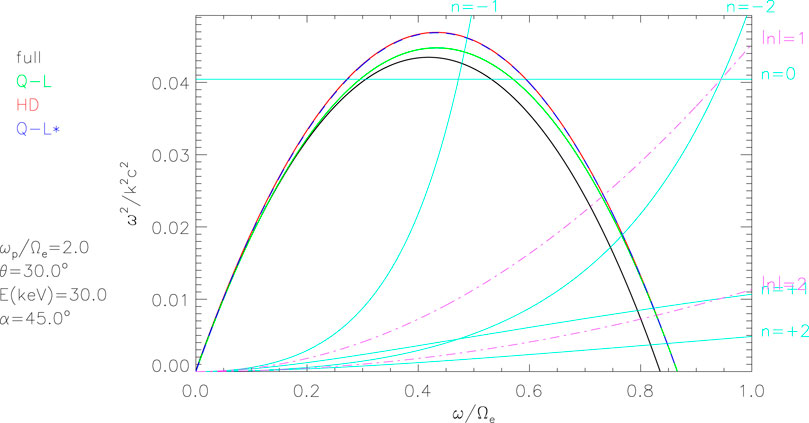
Figure 1. Versions of expressions constituting the resonance condition, for the parameter values shown in the plot. The inverted-U-shaped curves are the inverse-squared refractive index, given by Equation 5 (black), 7 (green), 11 (red), or 12 (blue). The upward-sloping (or horizontal) cyan curves show the corresponding term of the resonance condition (right-hand side of Equation 4) for several values of the harmonic number
2.2 Quasi-longitudinal approximation
From Equation 5, the quasi-longitudinal approximation neglects the terms proportional to
which is illustrated in Figure 1. With
with
With
With
If
2.3 High-density approximation
Lyons (1974b) and Albert (1999) used “high-density approximation,” which amounts to neglecting the leading term 1 relative to the terms proportional to
which is illustrated in Figure 1. A similar form applies to L-mode EMIC waves. Equation 11 should be accurate for a wider range of
Setting
which was used by Albert (2017) in a treatment of highly oblique whistler waves. It can also be regarded as a simplified version of quasi-longitudinal approximation. Combining it with the resonance condition yields a cubic equation of the form of Equation 8 with
This set of coefficients agrees exactly with Equation 9 for
2.4 Approximate resonance condition
Lyons et al. (1972) and Albert (1994) considered
and further approximated the refractive index (Equation 12) as
Both of these approximations are illustrated in Figure 1. At the risk of discarding two potential “anomalous” resonances with
However, combining Equation 14 with Equation 11, instead of the cruder approximation Equation 15, replaces Equation 16 with a quadratic equation for
2.5 Compensating changes in R and energy
The various expressions in the preceding sections all suggest that the resonant frequency
The scaling for
Equation 17 might further suggest that both the local pitch angle
The dependence on
Thus, with
Longley et al. (2022) used this expression with
For
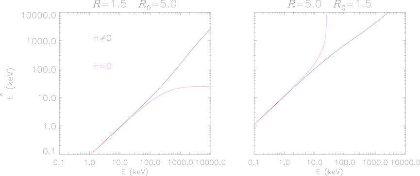
Figure 2. Values of
3 Diffusion coefficients
Even when
Using the expressions and notation of Albert (2005) and Albert (2007b) (which are exactly equivalent to those in Glauert and Horne (2005)), the local pitch angle diffusion coefficient is
where
Furthermore, from Lyons (1974a),
Note that
To characterize
so the factor of
The factor
The overall scaling of Equation 21 is therefore,
Thus, if
which refines Equation 20. Similarly, using Equations 23, 25, taking
Mourenas and Ripoll (2012) and Artemyev et al. (2013), relying on the refractive index of Equation 15 and approximations of
4 Numerical tests
Bounce-averaged quasi-linear diffusion coefficients were calculated using the simple chorus wave models of Glauert and Horne (2005) and Horne et al. (2005), namely,
The parameter values used in Equation 29 are
The top panel of Figure 3 shows values of
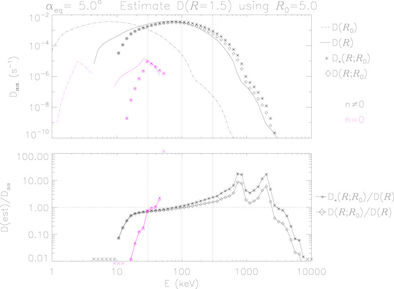
Figure 3. Calculated and estimated values of
The comparison is made clearer in the bottom panel of Figure 3, which shows the ratios of estimated to calculated values. For
The results of conversely using values calculated for
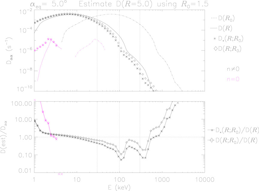
Figure 4. Calculated and estimated values of
Figures 5, 6 repeat Figures 3, 4 using the mid-latitude chorus model. With
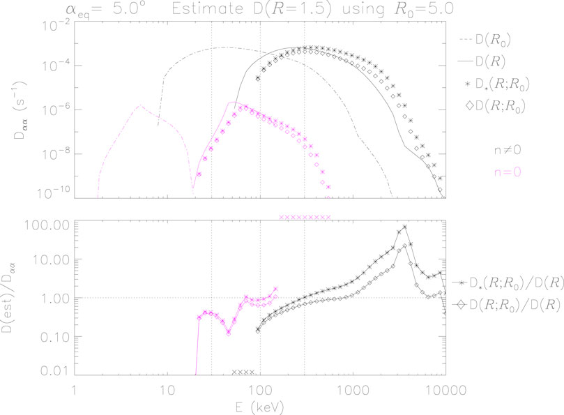
Figure 5. Calculated and estimated values of
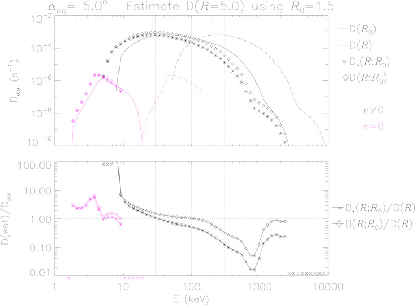
Figure 6. Calculated and estimated values of
Figure 7 shows equatorial pitch angle diffusion coefficients for the equatorial chorus model as a function of both energy and pitch angle. Calculated values of
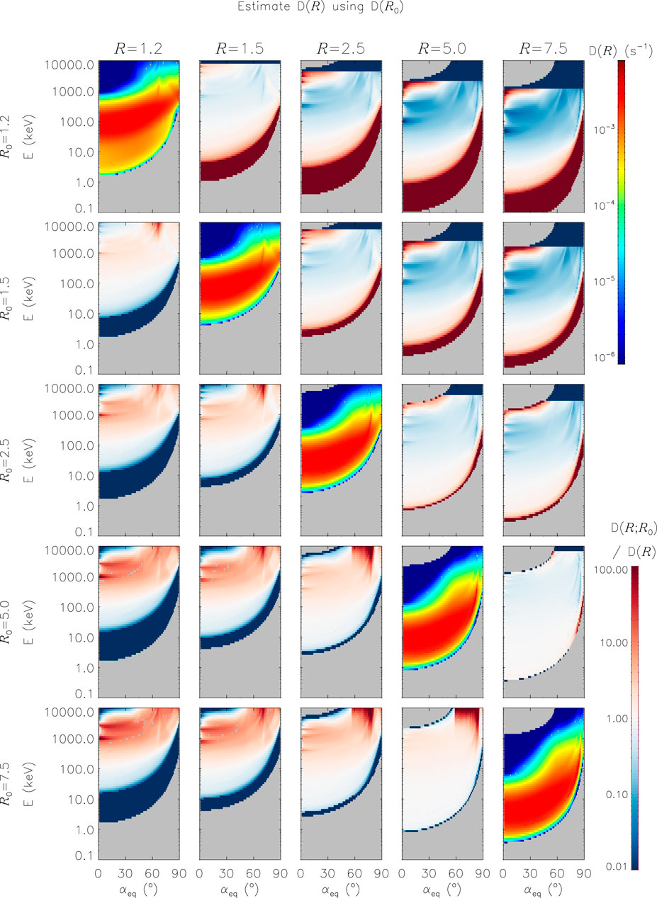
Figure 7. Calculated and estimated values of

Figure 8. Same as Figure 7 but for mid-latitude chorus waves.
5 Summary
This paper explored a method for quickly and easily estimating bounce-averaged quasi-linear diffusion coefficients for one value of “density ratio”
Although the original derivation was justified on the basis of parallel-propagating waves (wave normal angle
The resulting agreement is far from perfect, however, especially when
We note that all parameters specifying the wave frequency and wave normal angle distributions have been held fixed throughout. Sensitivity to these parameters was considered by Albert (2012). Furthermore, the quasi-linear diffusion paradigm itself has well-known caveats and limitations, e.g., Allanson et al. (2024). For use with the POES technique, which has additional sources of inaccuracy and uncertainty, the estimates here are probably acceptable. If nothing else, the wave amplitude and density values obtained can be used in more refined calculations. More generally, the tradeoff of accuracy for computational convenience should be carefully assessed for each intended application. One possible avenue toward improvement is to precompute several tables of diffusion coefficients, with different values of
Data availability statement
The original contributions presented in the study are included in the article/supplementary material; further inquiries can be directed to the corresponding author.
Author contributions
JA: conceptualization, formal analysis, methodology, software, and writing–original draft. WL: conceptualization, formal analysis, and writing–review and editing. AC: conceptualization and writing–review and editing.
Funding
The author(s) declare that financial support was received for the research, authorship, and/or publication of this article. JA was supported by the AFOSR grant 2021RVCOR002 and the Space Vehicles Directorate of the Air Force Research Laboratory. WL and AC acknowledge the NASA grant 80NSSC21K1323.
Acknowledgments
The views expressed are those of the author and do not necessarily reflect the official policy or position of the Air Force, the Department of Defense, or the U. S. Government. The appearance of external hyperlinks does not constitute endorsement by the United States Department of Defense (DoD) of the linked websites, or the information, products, or services contained therein. The DoD does not exercise any editorial, security, or other control over the information one may find at these locations.
Conflict of interest
The authors declare that the research was conducted in the absence of any commercial or financial relationships that could be construed as a potential conflict of interest.
Publisher’s note
All claims expressed in this article are solely those of the authors and do not necessarily represent those of their affiliated organizations, or those of the publisher, the editors, and the reviewers. Any product that may be evaluated in this article, or claim that may be made by its manufacturer, is not guaranteed or endorsed by the publisher.
References
Albert, J. M. (1994). Quasi-linear pitch angle diffusion coefficients: retaining high harmonics. J. Geophys. Res. 99 (23), 23741–23745. doi:10.1029/94JA02345
Albert, J. M. (1999). Analysis of quasi-linear diffusion coefficients. J. Geophys. Res. 104, 2429–2441. doi:10.102910.1029/1998ja9001131998JA900113
Albert, J. M. (2003). Evaluation of quasilinear diffusion coefficients for emic waves in a multi-species plasma. J. Geophys. Res. 108, 1249. doi:10.1029/2002JA009792
Albert, J. M. (2004). Analytical bounds on the whistler mode refractive index. Phys. Plasmas 11, 4875–4877. doi:10.1063/.1.1792634
Albert, J. M. (2005). Evaluation of quasi-linear diffusion coefficients for whistler mode waves in a plasma with arbitrary density ratio. J. Geophys. Res. 110, A03218. doi:10.1029/2004JA010844
Albert, J. M. (2007a). Refractive index and wavenumber properties for cyclotron resonant quasilinear diffusion by cold plasma waves. Phys. Plasmas 14, 072901–1. doi:10.1063/1.2744363
Albert, J. M. (2007b). Simple approximations of quasilinear diffusion coefficients. J. Geophys. Res. 112, A12202. doi:10.1029/2007JA012551
Albert, J. M. (2008). Efficient approximations of quasilinear diffusion coefficients in the radiation belts. J. Geophys. Res. 113, A06208. doi:10.1029/2007JA012936
Albert, J. M. (2012). Dependence of quasilinear diffusion coefficients on wave parameters. J. Geophys. Res. Space Phys. 113, A09224. doi:10.1029/2012JA017718
Albert, J. M. (2017). Quasi-linear diffusion coefficients for highly oblique whistler mode waves. J. Geophys. Res. Space Phys. 122, 5339–5354. doi:10.1002/2017JA024124
Allanson, O., Ma, D., Osmane, A., Albert, J. M., Bortnik, J., Watt, C. E. J., et al. (2024). The challenge to understand the zoo of particle transport regimes during resonant wave-particle interactions for given survey-mode wave spectra. Front. Astron. Space Sci. 11, 1332931. doi:10.3389/.fspas/2024.1332931
Artemyev, A. V., Mourenas, D., Agapitov, O. V., and Krasnoselskikh, V. V. (2013). Parametric validations of analytical lifetime estimates for radiation belt electron diffusion by whistler waves. Ann. Geophys. 31, 599–624. doi:10.5194/angeo-31-599-2013
Chan, A. A., Elkington, S. R., Longley, W. J., Aldhurais, S. A., Alam, S. S., Albert, J. M., et al. (2023). Simulation of radiation belt wave-particle interactions in an MHD-particle framework. Front. Astron. Space Sci. 10, 1239160. doi:10.3389/fspas.2023.1239160
Glauert, S. A., and Horne, R. B. (2005). Calculation of pitch angle and energy diffusion coefficients with the PADIE code. J. Geophys. Res. 110, A04206. doi:10.1029/2004JA010851
Horne, R. B., Thorne, R. M., Glauert, S. A., Albert, J. M., Meredith, N. P., and Anderson, R. R. (2005). Timescale for radiation belt electron acceleration by whistler mode chorus waves. J. Geophys. Res. 110, A03225. doi:10.1029/.2004JA010811
Kennel, C. F., and Engelmann, F. (1966). Velocity space diffusion from weak plasma turbulence in a magnetic field. Phys. Fluids 9, 2377–2388. doi:10.1063/1.1761629
Lerche, I. (1968). Quasilinear theory of resonant diffusion in a magneto-active, relativistic plasma. Phys. Fluids 11, 1720–1727. doi:10.1063/1.1692186
Li, W., Ni, B., Thorne, R. M., Bortnik, J., Green, J. C., Kletzing, C. A., et al. (2013). Constructing the global distribution of chorus wave intensity using measurements of electrons by the POES satellites and waves by the Van Allen Probes. Geophys. Res. Lett. 40, 4526–4532. doi:10.1002/grl.50920
Longley, W. J., Chan, A. A., Jaynes, A. N., Elkington, S. R., Pettit, J. M., Ross, J. P., et al. (2022). Using MEPED observations to infer plasma density and chorus intensity in the radiation belts. Front. Astron. Space Sci. 9, 1063329. doi:10.3389/fspas.2022.1063329
Lyons, L. R. (1974a). General relations for resonant particle diffusion in pitch angle and energy. J. Plasma Phys. 12, 45–49. doi:10.1017/S0022377800024910
Lyons, L. R. (1974b). Pitch angle and energy diffusion coefficients from resonant interactions with ion-cyclotron and whistler waves. J. Plasma Phys. 12, 417–432. doi:10.1017/.S002237780002537X
Lyons, L. R., and Thorne, R. M. (1970). The magnetospheric reflection of whistlers. Planet. Space Sci. 18, 1753–1767. doi:10.1016/0032-0633(70)90009-7
Lyons, L. R., Thorne, R. M., and Kennel, C. F. (1971). Electron pitch angle diffusion driven by oblique whistler-mode turbulence. J. Plasma Phys. 6, 589–606. doi:10.1017/S0022377800006310
Lyons, L. R., Thorne, R. M., and Kennel, C. F. (1972). Pitch angle diffusion of radiation belt electrons within the plasmasphere. J. Geophys. Res. 77, 3455–3474. doi:10.1029/.JA077i019p03455
Michael, A. T., Sorathia, K. A., Ukhorskiy, A. Y., Albert, J., Shen, X., Li, W., et al. (2024). Cross-scale modeling of storm-time radiation belt variability. J. Geophys. Res. Space Phys. 129, e2023JA032175. doi:10.1029/2023JA032175
Mourenas, D., and Ripoll, J.-F. (2012). Analytical estimates of quasi-linear diffusion coefficients and electron lifetimes in the inner radiation belt. J. Geophys. Res. 117, A01204. doi:10.1029/2011JA016985
Ni, B., Li, W., Thorne, R. M., Bortnik, J., Green, J. C., Kletzing, C. A., et al. (2014). A novel technique to construct the global distribution of whistler mode chorus wave intensity using low-altitude POES electron data. J. Geophys. Res. Space Phys. 119, 5685–5699. doi:10.1002/2014JA019935
Watt, C. E. J., Allison, H. J., Thompson, R. L., Bentley, S. N., Meredith, N. P., Glauert, S. A., et al. (2021). The implications of temporal variability in wave-particle interactions in earth’s radiation belts. Geophys. Res. Lett. 48, e2020GL089962. doi:10.1029/2020GL089962
Keywords: wave–particle interactions, radiation belts, quasi-linear, diffusion, POES technique
Citation: Albert JM, Longley WJ and Chan AA (2024) Estimating quasi-linear diffusion coefficients for varying values of density ratio. Front. Astron. Space Sci. 11:1470742. doi: 10.3389/fspas.2024.1470742
Received: 26 July 2024; Accepted: 23 October 2024;
Published: 09 December 2024.
Edited by:
Xiao-Jia Zhang, The University of Texas at Dallas, United StatesReviewed by:
Adnane Osmane, University of Helsinki, FinlandMurong Qin, Boston University, United States
Copyright © 2024 Albert, Longley and Chan. This is an open-access article distributed under the terms of the Creative Commons Attribution License (CC BY). The use, distribution or reproduction in other forums is permitted, provided the original author(s) and the copyright owner(s) are credited and that the original publication in this journal is cited, in accordance with accepted academic practice. No use, distribution or reproduction is permitted which does not comply with these terms.
*Correspondence: Jay M. Albert, amF5LmFsYmVydEBzcGFjZWZvcmNlLm1pbA==