 J. D. Huba
- Syntek Technologies, Fairfax, VA, United States
The impact of meridional winds on the onset and evolution of equatorial plasma bubbles (EPBs) is reviewed. The conventional wisdom had been that transequatorial meridional winds have a stabilizing effect on the development of EPBs during equatorial spread F (ESF). However, this result is based on a uniform transequatorial meridional wind. Subsequently, it was demonstrated that a non-uniform meridional wind could have a stabilizing or destabilizing effect on EPB formation depending on the direction of wind gradient. The destabilization of EPBs associated with equatorward flowing meridional winds has recently been investigated during a midnight temperature maximum event and a geomagnetic storm. Although the neutral wind is a direct destabilizing influence in these cases, the large decrease in the Pedersen conductance caused by meridional equatorward winds is the primary reason for the large increase in the growth rate of the generalized Rayleigh-Taylor instability. We review the theoretical and modeling studies of this topic as well as observational studies that have been made to assess the relationship between meridional winds and ESF.
1 Introduction
The subject of the impact of meridional winds on the development of equatorial plasma bubbles (EPBs) has received considerable attention over the last 35 years (Huba and Krall, 2013; Huba et al., 2023; Huba and Lu, 2024). The generalized Rayleigh-Taylor instability (GRTI) (Sultan, 1996; Huba, 2022) is believed responsible for the generation of EPBs (Booker and Wells, 1938; Haerendel, 1974; Hysell, 2000) and a number of theoretical studies have focused on the impact of meridional winds on the GRTI to assess their role in EPB development.
The first study was performed by Maruyama (1988). He demonstrated that a uniform transequatorial meridional wind enhances the field-line integrated Pedersen conductivity and that this can reduce the growth rate of the generalized Rayleigh-Taylor instability. Zalesak and Huba (1991) extended the analysis of Maruyama (1988) to consider the direct effect of the wind on the development of the instability. They found that, in fact, the instability can be completely stabilized for a sufficiently strong meridional wind. These results were borne out in a 3D simulation study by Krall et al. (2009).
The work of Maruyama (1988) spurred interest in observational studies to assess the relationship between meridional winds and equatorial spread
A possible resolution to these “conflicting” observations was suggested by Huba and Krall (2013). They revisited this problem and demonstrated that a non-uniform meridional wind could have a stabilizing or destabilizing effect on EPB formation depending on the direction of wind gradient. Thus, the exact nature of the meridional wind is a key factor in how it affects the development of EPBs.
Recently, Huba et al. (2023) and Huba and Lu (2024) focused on equatorward flowing neutral winds and showed that they can be very destabilizing and generate EPBs. The primary reason for the large increase in the growth rate of the GRTI is a large decrease in the Pedersen conductivity. This is in contrast to the work of Maruyama (1988) who found that a uniform transequatorial meridional wind increased the Pedersen conductivity which led to a decrease in the growth rate of the GRTI.
We review the aforementioned theoretical and modeling studies, as well as the observational studies relating measurements of the meridional wind to the onset and evolution of ESF.
2 Theory
The theory of the stabilizing effects of meridional winds on the Rayleigh-Taylor instability was first developed by Maruyama (1988) and expanded upon by Zalesak and Huba (1991). Krall et al. (2009) elaborated on the theory and confirmed the stabilizing influence of meridional winds on the GRTI through numerical simulation studies using SAMI3/ESF (Huba et al., 2008). Recently, a more thorough analysis of the GRTI was presented by Huba (2022).
where
and
with
Gravity being directed downwards,
In Figure 1 we show a schematic indicating the important factors that affect the growth rate of the Rayleigh-Taylor instability associated with a meridional wind. In this figure we show a meridional wind (dark blue vector) in the northward direction and an upward density gradient (dark green vector) in the bottomside
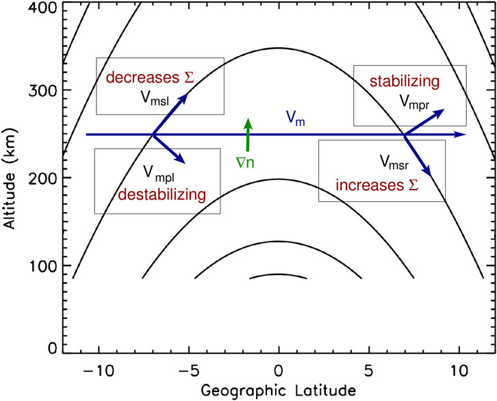
Figure 1. Schematic of the impact of meridional wind components on the growth rate and conductivity.
First, the component of the neutral wind along the geomagnetic field
Second, the component of the neutral wind transverse to the geomagnetic field
3 Modeling
Krall et al. (2009) performed an extensive simulation study of the impact of the meridional wind on the development of equatorial plasma bubbles (EPBs). They used a constant transhemispheric meridional wind and their results confirmed the results of Maruyama (1988) and Zalesak and Huba (1991). As an example we show Figure 2 which plots the maximum vertical E
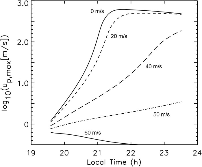
Figure 2. Line plots showing
Huba and Krall (2013) expanded the previous work of Krall et al. (2009) to include an inhomogeneous meridional wind; they demonstrated that, depending on the direction of the latitudinal gradient of the wind, the meridional wind could be stabilizing or destabilizing. Specifically, a wind profile with a positive gradient as a function of latitude
As “extreme” cases, they considered equatorward flowing winds
where
The results are shown in Figure 3 where the labels
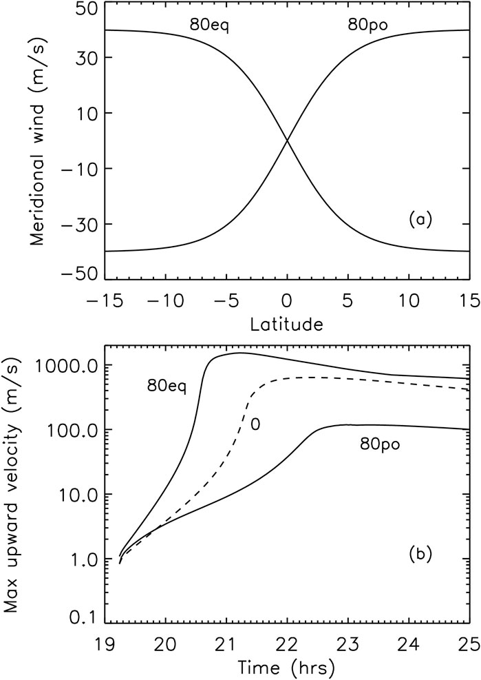
Figure 3. Plots of (A) the meridional neutral wind profiles as a function of latitude for
The contrast in the development of the generalized Rayleigh-Taylor instability for the equatorward and poleward meridional wind cases is exemplified in Figure 4. Electron density contours are shown at time
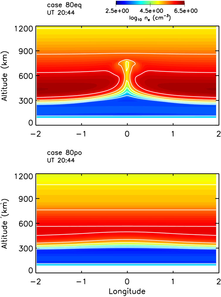
Figure 4. Contour plots of the electron density at time
The modeling results described above were based on the SAMI3/ESF code (Huba et al., 2008) which models a narrow range of longitude at night; nominally about
Huba et al. (2023) investigated the development of an EPB during a period of low geomagnetic activity at solar minimum near the summer solstice using the coupled SAMI3/WACCM-X code. The parameters used were for August 22 with F10.7 = 71.6, F10.7A = 72.4, Ap = 6 and Kp = 1. The role of the meridional wind on the EPB growth is highlighted in Figure 5 which shows contour plots of the electron density (a, b), E × B velocity (c, d), zonal neutral wind (e, f), meridional neutral wind (g, i), latitude derivative of the meridional neutral wind (h, j), and neutral temperature (k, l) at times 11:59 UT (left panels) and 12:29 UT (right panels) as a function of latitude and altitude at longitude
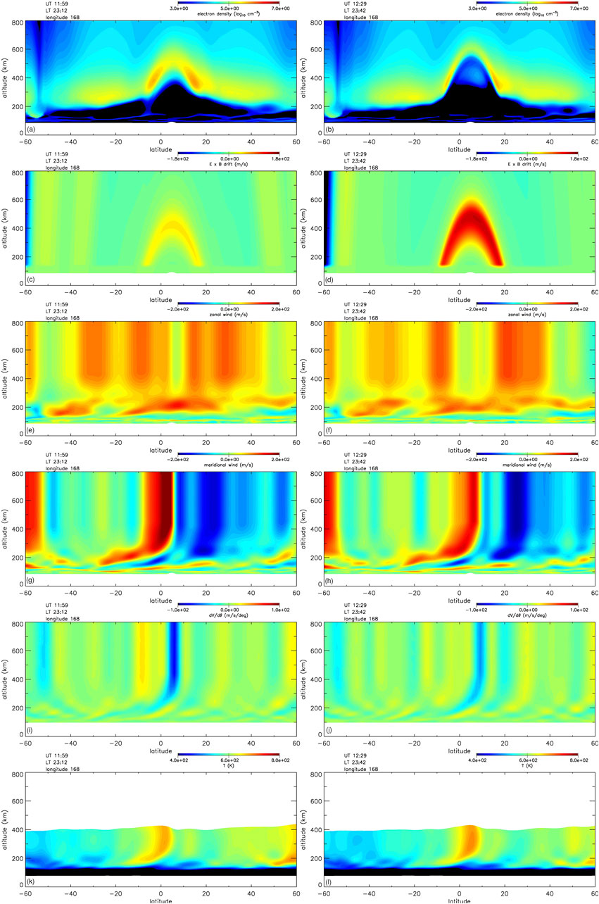
Figure 5. Contour plots of the electron density (A, B), E
The reason for the development of the EPB in Figure 5 is described in Figure 6 from Huba et al. (2023). This figure shows line plots of the (a) electron density
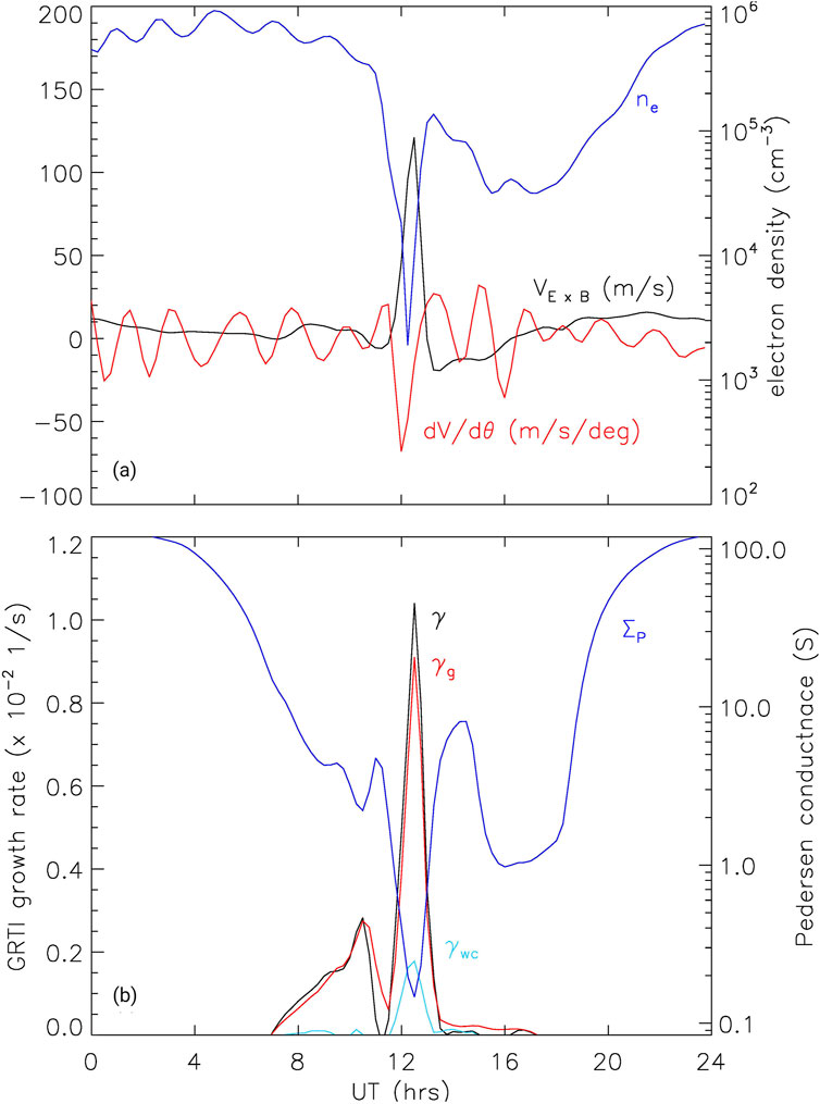
Figure 6. Line plots of (A) the electron density
The aforementioned simulation study was for quiet geomagnetic conditions and generated a single EPB that rose to
The simulation used the coupled SAMI3/WACCM-X code to model the days 6–8 September 2017. The geophysical parameters considered are F10.7 = 134.9, 130.4, 118.5, F10.7A = 84.3, 84.3, 84.3, and Ap = 8, 36, 106 for each day, respectively. In Figure 7 contour plots of the electron density (a, e), meridional wind (b, f), E
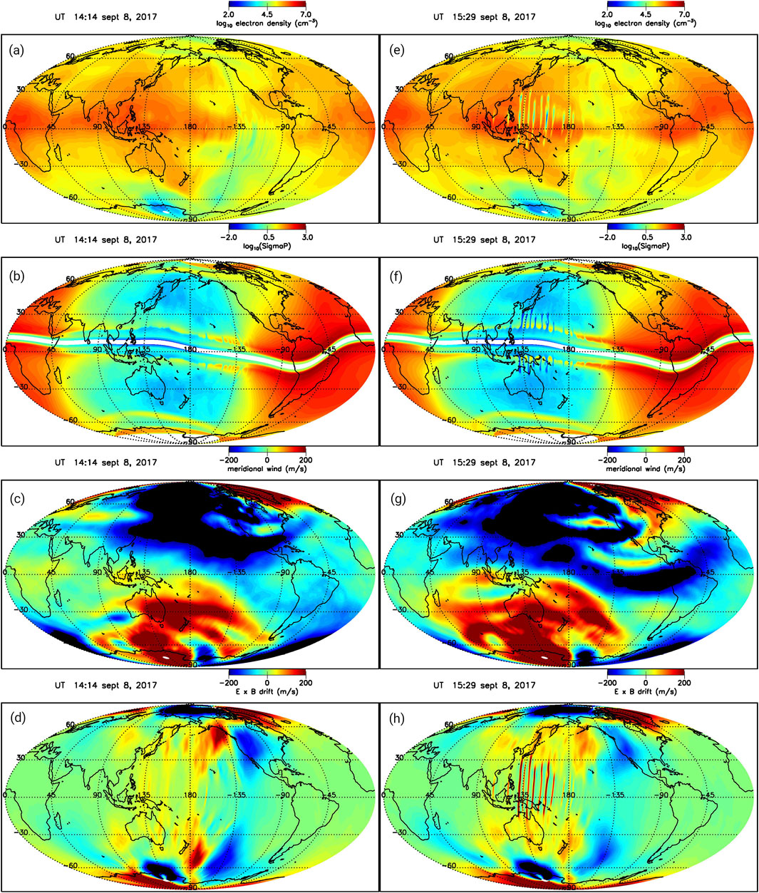
Figure 7. Contour plots of the electron density (A, E), meridional wind (B, F), E
Figures 7E–H correspond to Figures 7A–D but 75 min later at 15:29 UT. The equatorward meridional winds in Figure 7F have become more intense closer to the equator as well as a reduction in the Pedersen conductance at low- to mid-latitudes. However, the most striking features that have developed are shown in Figures 7E, H. In Figure 7E a span of EPBs developed in the longitude range
4 Observations
The initial observational studies of the relationship between transhemispheric meridional winds and ESF focused on the suppression of ESF because of the work by Maruyama (1988). Mendillo et al. (1992) performed a two-day case study using the ALTAIR radar and optical imaging data. They found that ESF was suppressed on the first night (14 August 1988) but not the next night (15 August 1988). They attribute the suppression of ESF on the first night to a north-to-south meridional wind based on a reduction of the northern meridional gradient in 6,300 Å airglow. A subsequent study by Mendillo et al. (2001) during the Multi-Instrumented Studies of Equatorial Thermospheric Aeronomy (MISETA) campaign found “no convincing evidence for the wind suppression mechanism.”
Thampi et al. (2006) developed a prediction parameter
Maruyama et al. (2007) developed an ionosonde network in the Southeast Asian sector consisting of a meridional chain and a pair near the equator designed to estimate the meridional wind based on nighttime ionospheric height variations. Maruyama et al. (2009) used this network to infer the meridional winds for the spring and fall equinoxes in 2004 and 2005, and correlated the results with the occurrence of equatorial irregularities. They found that the transequatorial meridional winds were larger in September than March, and suggested that this was why equatorial irregularities occurred less frequently in September than in March. Numerical simulations were performed using the SAMI3/ESF model to support this contention. A Brazilian study during 1999 and 2001 by Abdu et al. (2006) also concluded that magnetic meridional winds negatively influence ESF development by reducing the pre-reversal enhancement electric field and direct suppression of the instability.
On the other hand, Devasia et al. (2002) and Jyoti et al. (2004) found that under certain circumstances equatorward neutral winds appeared to be needed for ESF to develop. Specifically, Devasia et al. (2002) argued that when the h’F base height of the
Sreekumar and Sripathi (2016), Sreekumar and Sripathi (2017) studied nighttime thermospheric meridional winds in the Indian sector during the period March–December 2013. They derived the wind structure based on the h’F and hpF2 methods using ionosonde data. Comparing the results of the two methods to the HWM07 empirical wind model, it was found that the h’F was in better agreement. They related their h’F wind measurements to GPS scintillation data (i.e., an indicator of equatorial spread
Gao et al. (2023) studied the relationship between geomagnetic substorms and the occurrence of equatorial spread
Zhan and Rodrigues (2018) investigated the dynamics of equatorial spread
5 Discussion
Although not surprising, the results of this paper highlight the potential importance of meridional neutral winds in the development of EPBs during equatorial spread
It also appears meridional winds can play a dramatic role in the development of large-scale EPBs during magnetic storms (Gao et al., 2023; Huba and Lu, 2024). During geomagnetic storms, heating of the thermosphere at high-latitude generates strong modifications to both the zonal and meridional winds that propagates equatorward over a period of several hours. This can lead to an upward E
The dominant theme of this review is that meridional winds can affect the onset and evolution of EPBs during ESF, primarily by modification of the conductance which directly impacts the growth rate of the GRTI. This doesn’t necessarily obviate the possibility of other factors playing a roll such as seeding mechanisms (e.g., gravity waves), modification of the lower
We also note that Kherani et al. (2005) presented a theoretical and modeling study of the collisional interchange instability. In this work a linear, local analysis was performed that considered a 3D potential equation (in contrast to the current analysis which assumes equipotential field lines). They found that a meridional wind can generate a density gradient along the magnetic field line that has a stabilizing influence on the instability when considering parallel oscillations (e.g.,
In conclusion, additional measurements of the neutral wind, in conjunction with observations of EPBs and ESF, are needed to provide a clearer understanding of ESF onset and evolution, and in particular the day-to-day variability of ESF. To this end the Ionospheric Connections Explorer (ICON) satellite mission data provides an invaluable resource for neutral wind and plasma data to address this problem (Immel et al., 2018).
Author contributions
JH: Writing–original draft, Writing–review and editing.
Funding
The author(s) declare that financial support was received for the research, authorship, and/or publication of this article. This research was supported by NASA grants 80NSSC21K1305, ICON Explorers Program through contracts NNG12FA45C and NNG12FA42I, and DRIVE Science Center for Geospace Storms (CGS) under award (80NSSC22M0163), and AFOSR (FA9550-22-C-0001).
Conflict of interest
Author JH is employed by Syntek Technologies.
The author(s) declared that they were an editorial board member of Frontiers, at the time of submission. This had no impact on the peer review process and the final decision.
Publisher’s note
All claims expressed in this article are solely those of the authors and do not necessarily represent those of their affiliated organizations, or those of the publisher, the editors and the reviewers. Any product that may be evaluated in this article, or claim that may be made by its manufacturer, is not guaranteed or endorsed by the publisher.
References
Abdu, M. A., Iyer, K. N., de Medeiros, R. T., Batista, I. S., and Sobral, J. H. A. (2006). Thermospheric meridional wind control of equatorial spread F and evening prereversal electric field. Geophys. Res. Lett. 33, L07106. doi:10.1029/2005GL024835
Booker, H. G., and Wells, H. G. (1938). Scattering of radio waves by the F-region of the ionosphere. Terr. Mag. Atmos. Elec. 43, 249–256. doi:10.1029/te043i003p00249
Devasia, C. V., Jyoti, N., Viswanathan, K. S., Tiwari, D., and Sridharan, R. (2002). On the plausible linkage of thermospheric meridional winds with equatorial spread F. J. Atmos. Sol. Terr. Phys. 64 (1), 1–12. doi:10.1016/s1364-6826(01)00089-x
Gao, S., Cail, H., Zhan, W., Wan, X., Xiong, C., Zhang, H., et al. (2023). Characterization of local time dependence of equatorial spread F responses to substorms in the American sector. J. Space Weather Space Clim. 13 (2), 2. doi:10.1051/swsc/2022039
Haerendel, G. (1974). Theory of equatorial spread F, Munich, Germany: Max Planck Institute for Extraterrestrial Physics.
Heelis, R. A., Stoneback, R., Earle, G. D., Haaser, R. A., and Abdu, M. A. (2010). Medium-scale equatorial plasma irregularities observed by coupled ion-neutral dynamics investigation sensors aboard the communication navigation outage forecast system in a prolonged solar minimum. Ionosphere and Upper Atmosphere 115, A10321. doi:10.1029/2010JA015596
Herrero, F. A., Spencer, N. W., and Mayr, H. G. (1993). Thermosphere and F-region plasma dynamics in the equatorial region. Adv. Space Res. 13, 201–220. doi:10.1016/0273-1177(93)90019-8
Huba, J. D., Joyce, G., and Fedder, J. A. (2000). SAMI2 (Sami2 is another model of the Ionosphere): a new low-latitude Ionosphere model. J. Geophys. Res. 105, 23035
Huba, J. D., Joyce, G., and Krall, J. (2008). Three-dimensional equatorial spread F modeling. Geophys. Res. Lett. 35, L10102. doi:10.1029/2008GL033509
Huba, J. D., and Joyce, G. (2010). Global modeling of equatorial plasma bubbles. Geophys. Res. Lett. 37, L17104. doi:10.1029/2010GL044281
Huba, J. D., and Krall, J. (2013). Impact of meridional winds on equatorial spread F: revisited. Geophys. Res. Lett. 40, 1268–1272. doi:10.1002/grl.50292
Huba, J. D., and Liu, H.-L. (2020). Global modeling of equatorial spread F with SAMI3/WACCM-X. Geoophy. Res. Lett. 47, e2020GL088258. doi:10.1029/2020GL088258
Huba, J. D. (2022). Generalized Rayleigh-Taylor instability: ion inertia, acceleration forces, and E region drivers. J. Geophys. Res. Space Phys. 127, e2022JA030474. doi:10.1029/2022JA030474
Huba, J. D., Liu, H.-L., and McInerney, J. (2023). Modeling the development of an equatorial plasma bubble during a midnight temperature maximum with SAMI3/WACCM-X. Geoophy. Res. Lett. 50, e2023GL104388. doi:10.1029/2023GL104388
Huba, J. D., and Lu, G. (2024). Modeling equatorial plasma bubbles with Sami3/WACCM-X september 2017 storm. Geophys. Res. Lett. 5, e2024GL109071. doi:10.1029/2024GL109071
Hysell, D. L. (2000). An overview and synthesis of plasma irregularities in equatorial spread F. J. Atmos. Sol. Terr. Phys. 62, 1037–1056. doi:10.1016/s1364-6826(00)00095-x
Hysell, D. L., Milla, M. A., Condori, L., and Vierinen, J. (2015). Data-driven numerical simulations of equatorial spread F in the Peruvian sector 3: solstice. J. Geophys. Res. Space Phys. 120 (10)–809. doi:10.1002/2015JA021877
Immel, T. J., England, S. L., Mende, S. B., Heelis, R. A., Englert, C. R., Edelstein, J., et al. (2018). The ionospheric connection explorer mission: mission goals and design. Space Sci. Rev. 214, 13. doi:10.1007/s11214-017-0449-2
Jyoti, N., Devasia, C. V., Sridharan, R., and Tiwari, D. (2004). Threshold height (h’F)c for the meridional wind to play a deterministic role in the bottom side equatorial spread F and its dependence on solar activity. Geophys. Res. Lett. 31, L12809. doi:10.1029/2004GL019455
Kherani, A. E., Mascarenhas, M., de Paula, E. R., Sobral, J. H. A., and Bertoni, F. (2005). A three-dimensional simulation of collisional-interchange-instability in the equatorial-low-latitude ionosphere. Space Sci. Rev. 121, 253–269. doi:10.1007/s11214-006-6158-x
Krall, J., Huba, J. D., Joyce, G., and Zalesak, S. T. (2009). Three-dimensional simulation of equatorial spread F with meridional wind effects. Ann. Geophys. 27, 1821–1830. doi:10.5194/angeo-27-1821-2009
Li, G., Ning, B., Abdu, M. A., Yue, X., Liu, L., Wan, W., et al. (2011). On the occurrence of postmidnight equatorial F region irregularities during the June solstice. J. Geophys. Res. 116, A04318. doi:10.1029/2010JA016056
Liu, H. L., Bardeen, C. G., Foster, B. T., Lauritzen, P., Liu, J., and Lu, G. (2018). Development and validation of the whole atmosphere community climate model with thermosphere and ionosphere extension (WACCM-X 2.0). J. Adv. Model. Earth Sys. 10, 381. doi:10.1002/2017MS001233
Maruyama, T. (1988). A diagnostic model for equatorial spread F, 1, Model description and application to electric field and neutral wind effects. J. Geophys. Res. 93 (14), 14611–14622. doi:10.1029/ja093ia12p14611
Maruyama, T., Kawamura, M., Saito, S., Nozaki, K., Kato, H., Hemmakorn, N., et al. (2007). Low latitude ionosphere-thermosphere dynamics studies with inosonde chain in Southeast Asia. Ann. Geophys. 25, 1569–1577. doi:10.5194/angeo-25-1569-2007
Maruyama, T., Saito, S., Kawamura, M., Nozaki, K., Krall, J., and Huba, J. D. (2009). Equinoctial asymmetry of a low-latitude ionosphere-thermosphere system and equatorial irregularities: evidence for meridional wind control. Ann. Geophys. 27, 2027–2034. doi:10.5194/angeo-27-2027-2009
Mendillo, M., Baumgardner, J., Pi, X., Sultan, P., and Tsunoda, R. (1992). Onset conditions for equatorial spread F. J. Geophys. Res. 97 (13), 13865–13876. doi:10.1029/92ja00647
Mendillo, M., Meriwether, J., and Biondi, M. (2001). Testing the thermospheric neutral wind suppression mechanism for day-to-day variability of equatorial spread F. J. Geophys. Res. 106, 3655–3663. doi:10.1029/2000ja000148
Meriwether, J., Faivre, M., Fesen, C., Sherwood, P., and Veliz, O. (2008). New results on equatorial thermospheric winds and the midnight temperature maximum. Ann. Geophys. 26, 447–466. doi:10.5194/angeo-26-447-2008
Newell, P. T., and Gjerloev, J. W. (2011). Evaluation of SuperMAG auroral electrojet indices as indicators of substorms and auroral power. J. Geophys Res. Space Phys. 116. doi:10.1029/2011JA016779
Scherliess, L., and Fejer, B. (1999). Radar and satellite global equatorial F region vertical drift model. J. Geophys. Res. 104, 6829–6842. doi:10.1029/1999ja900025
Sekar, R., and Raghavarao, R. (1987). Role of vertical winds on the Rayleigh-Taylor mode instabilities of the night-time equatorial ionosphere. J. Atmos. Terr. Phys. 49, 981–985. doi:10.1016/0021-9169(87)90104-8
Sreekumar, S., and Sripathi, S. (2016). Nighttime thermospheric meridional winds as inferred from ionosonde parameters over Indian region and their plausible effects on plasma irregularities. Adv. Space Res. 58 (92), 92–107. doi:10.1016/j.asr.2016.04.009
Sreekumar, S., and Sripathi, S. (2017). A seasonal study on the role of h’F/meridional winds in influencing the development of ESF irregularities over Indian sector. Adv. Space Res. 60, 652–666. doi:10.1016/j.asr.2017.04.009
Sultan, P. J. (1996). Linear theory and modeling of the Rayleigh-Taylor instability leading to the occurrence of equatorial spread F. J. Geophys. Res. 101 (26), 26875–26891. doi:10.1029/96ja00682
Thampi, S. V., Ravindran, S., Pant, T. K., Devasia, C. V., Sreelatha, P., and Sridharan, R. (2006). Deterministic prediction of post-sunset ESF based on the strength and asymmetry of EIA from ground based TEC measurements: preliminary results. Geophys. Res. Lett. 33, L13103. doi:10.1029/2006GL026376
Zalesak, S. T., and Huba, J. D. (1991). Effect of meridional winds on the development of equatorial spread F. Eos Trans. AGU 72, Spring Meet. Suppl. 211.
Zhan, W., Rodrigues, F., and Milla, M. (2018). On the genesis of postmidnight equatorial spread F: results for the American/Peruvian sector. Geophys. Res. Lett. 45, 7354–7361. doi:10.1029/2018GL078822
Keywords: equatorial plasma bubbles, meridional wind, equatorial irregularities, equatorial spread F, generalized Rayleigh-Taylor instability
Citation: Huba JD (2024) Impact of meridional winds on the development of equatorial plasma bubbles: a review. Front. Astron. Space Sci. 11:1472642. doi: 10.3389/fspas.2024.1472642
Received: 29 July 2024; Accepted: 23 September 2024;
Published: 11 October 2024.
Edited by:
Marco Milla, Pontifical Catholic University of Peru, PeruReviewed by:
Yun Gong, Wuhan University, ChinaTatsuhiro Yokoyama, Kyoto University, Japan
Esfhan Alam Kherani, National Institute of Space Research (INPE), Brazil
Copyright © 2024 Huba. This is an open-access article distributed under the terms of the Creative Commons Attribution License (CC BY). The use, distribution or reproduction in other forums is permitted, provided the original author(s) and the copyright owner(s) are credited and that the original publication in this journal is cited, in accordance with accepted academic practice. No use, distribution or reproduction is permitted which does not comply with these terms.
*Correspondence: J. D. Huba, amRodWJhQGdtYWlsLmNvbQ==