Modeling exospheres: analytical and numerical methods with application examples

Exospheres, the tenuous gas environments surrounding planets, planetary satellites, and cometary comae, play a significant role in mediating the interactions of these astronomical bodies with their surrounding space environments. This paper presents a comprehensive review of both analytical and numerical methods employed in modeling exospheres. The paper explores analytical models, including the Chamberlain and Haser models, which have significantly contributed to our understanding of exospheres of planets, planetary satellites, and cometary comae. Despite their simplicity, these models provide baselines for more complex simulations. Numerical methods, particularly the Direct Simulation Monte Carlo (DSMC) method, have proven to be highly effective in capturing the detailed dynamics of exospheres under non-equilibrium conditions. The DSMC method’s capacity to incorporate a wide range of physical processes, such as particle collisions, chemical reactions, and surface interactions, makes it an indispensable tool in planetary science. The Adaptive Mesh Particle Simulator (AMPS), which employs the DSMC method, has demonstrated its versatility and effectiveness in simulating gases in planetary and satellite exospheres and dusty gas cometary comae. It provides a detailed characterization of the physical processes that govern these environments. Additionally, the multi-fluid model BATSRUS has been effective in modeling neutral gases in cometary comae, as discussed in the paper. The paper presents methodologies of exosphere modeling and illustrates them with specific examples, including the modeling of the Enceladus plume, the sodium exosphere of the Moon, the coma of comet 67P/Churyumov-Gerasimenko, and the hot oxygen corona of Mars and Venus.

1 Introduction

Exospheres, the outermost layers of a planet’s atmosphere, are critical for understanding the interactions between celestial bodies and their surrounding space environment. These tenuous atmospheres, often composed of light elements and molecules, play significant roles in shaping the observable characteristics of planets, moons, and comets. The study of exospheres encompasses various phenomena, including the dynamics of escaping particles, photochemical reactions, and interactions with solar wind.

Early analytical models like the Chamberlain and Haser models are fundamental for understanding exospheric structures. The Chamberlain model, formulated in the 1960s, provides insights into the density distribution of planetary exospheres influenced by gravitational forces. It offers a theoretical framework to describe the distribution of particles in a collisionless regime, providing a robust model of the exospheres of planets and planetary satellites. In contrast, the Haser model, developed for comets, focuses on the spatial distribution of neutral gas molecules and their photodissociation products. It has been instrumental in analyzing cometary comae and understanding the composition and distribution of gas species within them.

Despite their simplicity, these analytical models continue to serve as foundational tools in planetary science. They offer efficient means for initial data analysis and provide baselines for more complex numerical simulations. The emergence of high-resolution observations and sophisticated numerical methods, such as the Direct Simulation Monte Carlo (DSMC) method, have significantly advanced our understanding of exospheres. These methods allow for detailed simulations of gas flows under non-equilibrium conditions, capturing a broad range of physical processes, including particle collisions, chemical reactions, and interactions with surfaces for surface-bound exospheres and thermospheres of planets with substantial atmospheres.

2 Analytical models

Today, analytic models continue to be used, especially in analyzing observational data, preceding more complicated numerical modeling that accounts for detailed physics. Though lacking some physics, these models offer an efficient framework for performing an initial analysis, capturing the main physical processes. This section includes some of the analytic models, intending to provide the reader with a starting point for applying them in the analysis of observational data.

Initially formulated in the 1960s, the Chamberlain model was developed to describe planetary exospheres’ density distribution. It considers the thermal distribution of particles escaping from the gravitational field, providing insights into the exospheric dynamics and particle behavior (Shen, 1963; Chamberlain, 1963). In contrast, the Haser model, introduced in the 1950s, was specifically developed to model the coma of comets. This model describes the spatial distribution of neutral gas molecules and their photodissociation products (Haser, 1957). Cassini’s discovery of Enceladus’s jet produced by a combination of individual gas vents and Tiger stripes motivated the development of a multi-plume model (Tenishev et al., 2014).

2.1 Chamberlain model

Developed by Chamberlain (1963), this model provides insights into the density distribution in planetary exospheres influenced by planetary gravity. TheThe model assumes a Maxwellian velocity distribution at the base of a spherically symmetric exosphere, where particles are injected. he formalism of the model is discussed in detail, e.g., Shen (1963), Chamberlain (1963), Stern and Flynn (1995), Lammer and Bauer (1997), Valeille (2009), and Öpik and Singer (1961). Despite its limitations, the Chamberlain model remains instrumental in studying the evolution of planetary atmospheres.

Assuming that (1) the exosphere is spherically symmetric, and (2) at the location of the exobase, which serves as the lower boundary for the model, the atmosphere is in equilibrium, the density in the entire exosphere $n_a$ is in Equations 1, 2.

$\begin{array}{ll}\hfill n_a\left(r\right)& =n_0\left[e^{-\left(1-\alpha \right)E}-{\left(1-{\alpha }^2\right)}^{1/2}{e}^{-E/\left(1+\alpha \right)}\right]-\\ \hfill & n_0\left[\frac{{\alpha }^2}{2{\pi }^{1/2}}\frac{\left(1+E\right)e^{-E}}{E^{\frac{1}{2}}{\left[H\left(E\right)-1+\left[1-\frac{2}{3}H\left(E\right)\right]\alpha \right]}^{1/2}}\right],\hfill \end{array}(1)$

$H\left(E\right)=\frac{3}{2E}+\frac{1}{1+\frac{\sqrt{\pi }{e}^E}{\alpha E^{1/2}}\left[1-\text{erf}\left(\sqrt{E}\right)\right]}\approx 1+\frac{2}{E}\text{\hspace{0.17em}for\hspace{0.17em}large\hspace{0.17em}}E.(2)$

Here, $n_a$ is the density of a collisionless exosphere, $n_0$ is the density at the exobase, $E=\frac{GMm}{RkT}$, $\alpha =\frac{r_c}{r}$, where $r_c$ is the location of the exobase, and $T$ is the temperature at the exobase.

A traditional definition of the exobase’s location for an exosphere (Equation 3) is where the collision mean free path, $\lambda =\sigma n(r_c)$, equals the scale height, $H_{sh}$,

${\int }_{r_c}^{\infty }\sigma n\left(r\right)dr=\sigma n\left(r_c\right)H_{sh}\left(r_c\right)=\frac{H_{sh}\left(r_c\right)}{\lambda \left(r_c\right)}=1,(3)$

where $H_{sh}(r_c)=\frac{k{T}_0}{m{g}_0}$, and $\sigma$ is a total collision cross-section (Schunk and Nagy, 2000).

2.2 Haser model

Most radiative emissions of gaseous species in cometary comae, observable in visible light, are primarily due to fluorescence induced by sunlight within an optically thin medium. Quantitative analyses of gas species within these comae revealed that the spatial variation in the brightness of certain species (e.g., ${\mathrm{C}}_2$, CN) is inconsistent with the inverse distance relationship. Further investigations have recognized that most gas species detected through visible-range spectroscopy are not stable molecules but relatively unstable radicals produced by the photodissociation of parent molecules.

The quantitative framework for analyzing these phenomena, developed by Haser (1957), remains widely utilized in comet research today. Haser’s model characterizes the distribution of secondary species, such as cometary radicals, resulting from the photodissociation of parent species. The model assumes that the coma acts as a spherically symmetric point source from which parent molecules uniformly outflow. The depletion of these species’ densities, $n_p(r)$, is modeled using exponential decay:

$n_p\left(r\right)=\frac{Q}{4\pi r^{2}v}\left(e^{-r/{\gamma }_p}\right),(4)$

where Q is the production rate of the comet, $r$ is the distance from the nucleus, $v$ is the radial outflow speed, ${\gamma }_p=v/{\nu }_{ph}$ is the parent species scale lengths and ${\nu }_{ph}$ is the photo-destruction frequency. The density, $n_d$, of a daughter species created by the destruction of its parent species is given in Equation 5.

$n_d\left(r\right)=\frac{Q}{4\pi r^{2}v}\frac{{\gamma }_d}{{\gamma }_p-{\gamma }_d}\left(e^{-r/{\gamma }_p}-e^{-r/{\gamma }_d}\right)(5)$

Here, ${\gamma }_p$ is the daughter species scale lengths.

The processes occurring within the coma of a comet are generally more complex. Numerous daughter species detected do not originate from a singular, direct decomposition of a parent molecule. Instead, a daughter molecule may be produced from different parent molecules via diverse reaction pathways and may involve several intermediate stages. Moreover, if the dissociation processes are exothermic, the excess energy may enhance the reaction products’ kinetic energy, increasing the velocity of the lighter fragments (Shou, 2017; Combi et al., 2004). Despite its simplifications, the Haser model is extensively utilized as it provides a robust estimation of production rates by employing scale lengths readily available in the literature.

2.3 Multiplume model

The 2005 discovery by the Cassini spacecraft of gas and ice grain plumes emanating from Enceladus’ south pole has ignited significant interest in and research into the mechanisms behind these phenomena (Waite et al., 2006). The multiplume model developed to study the Enceladus’ plume integrates contributions from discrete gas vents, diffuse fissures or crevices along the Tiger Stripes - large, parallel cracks near the south pole that emit water vapor and ice particles and a global spherical source. The gas vents are treated as individual point sources where gas is ejected into the exosphere at high velocities (approximately 1 km/s), significantly exceeding Enceladus’ escape velocity (235 m/s) (Tenishev et al., 2014). Therefore, a number density of water vapor in the exosphere that is due to an individual gas vent can be evaluated as

$n\left(\mathbf{x}\right)=\left\{\begin{array}{c}\frac{A_p}{r^2}\int v^2\exp \left(-{\beta }^2\left[v^2{\sin }^2\theta +{\left(v\cos \theta -v_p\right)}^2\right]\right)dv\text{if}\left(\mathbf{x}-{\mathbf{r}}_p\right)\cdot {\mathbf{r}}_p\ge 0\hfill \\ 0\text{otherwise,}\hfill \end{array}\right.(6)$

where $\mathbf{x}$ is a point where a number density is calculated, $(r,\varphi ,\theta )$ are coordinates of the point $\mathbf{x}$ in a spherical coordinate frame associated with the vent, ${\mathbf{r}}_p$ is the vent location, $v_p$ is the bulk speed of the gas flow ejected from the vent, $\beta =\sqrt{\frac{m_{H_{2}O}}{2kT}}$, and $A_p$ is a normalization constant defined as

$A_p=\frac{F_p}{\iiint v^3\exp \left(-{\beta }^2\left[v^2{\sin }^2\theta +{\left(v\cos \theta -v_p\right)}^2\right]\right)dvd\theta d\varphi }(7)$

Here, $F_p$ is the total source rate $(s^{-1})$ of the vent. The integration limits in Equation 7 are constrained by the condition $(\mathbf{v}(v,\varphi ,\theta )\cdot {\mathbf{r}}_p)\ge 0$. Here, $\mathbf{v}$ is the velocity vector that corresponds to that defined in the spherical frame by the combinations of $(v,\varphi ,\theta )$. The integrals in Equations 6, 7 are calculated numerically.

3 Numerical modeling of exospheres

In planetary science, numerical modeling has become an essential tool for understanding the dynamics of exospheres of planets, moons, and comets. One of the most widely used numerical modeling techniques in this field is the Direct Simulation Monte Carlo (DSMC) method, a robust approach for solving the Boltzmann equation to simulate gas flows in exospheres. Despite the dominance of kinetic physics, fluid-type numerical methods are also employed for modeling exospheres due to their numerical efficiency and capabilities of being directly coupled with plasma models. This section provides an overview of both simulation methods.

3.1 Application of Monte Carlo method in exosphere simulations

In most cases of practical interest, studying exospheres of planets, planetary satellites, and comets involves rarefied gas flows under strong non-equilibrium conditions. These conditions can be described only with the Boltzmann equation, which, in its general form, can be written as

$\frac{\partial f_1}{\partial t}+{\mathbf{v}}_1\frac{\partial f_1}{\partial x}+{\mathbf{a}}_1\frac{\partial f_1}{\partial v_1}=\int |{\mathbf{v}}_1-{\mathbf{v}}_2|\left[f_1\left({\mathbf{v}}_1^{\prime }\right)f_1\left({\mathbf{v}}_2^{\prime }\right)-f_1\left({\mathbf{v}}_1\right)f_1\left({\mathbf{v}}_2\right)\right]d\sigma d{\mathbf{v}}_2,(8)$

where $\sigma$ is the scattering cross-section. The integral in the right-hand-side of Equation 8 describes collisions, by which collision partners having velocities ${\mathbf{v}}_1^{\prime }$ and ${\mathbf{v}}_2^{\prime }$ get the velocities ${\mathbf{v}}_1$ and ${\mathbf{v}}_2$ after the collision. Equation 8 can be generalized for gas mixtures and include the effect of external forces.

The Direct Simulation Monte Carlo (DSMC) method is a method of choice to solve the Boltzmann equation for gas flow in the exospheres of planets, moons, and comets (Combi, 1996; Tenishev et al., 2008; Bird, 1994; Crifo et al., 2002; Tucker et al., 2015). One of the DSMC method’s most important advantages is its ability to incorporate processes that are more complex than elastic collisions without significantly complicating the numerical procedure.

The general scheme of Monte Carlo models can be described using so-called Markov chains. Briefly, a Markov chain is defined as a system, $S$, consisting of a finite set of states $M\{s_1,s_2,\dots ,s_l\}$. At each discrete sequence of times $t=\mathrm{0,1,2},\dots ,n$, the system is in one of the states, $s_i$, which determines a set of conditional probabilities $p_{i1},p_{i2},\dots ,p_{il}$. The quantity $p_{ij}$ is the probability that the system, which is in state $s_i$ at the $n$-th time step, will be in state $s_j$ at the $(n+1)$-th time step. In other words, $p_{ij}$ is the probability of the transition $s_i\to s_j$. It is important to note that the probability of a transition depends only on the current state and is not affected by the previous history.

The evolution of the distribution function $f(\mathbf{v},t)$ as a Markov process is described by a collision integral

$f\left(\mathbf{v},t\right)=\int f\left(\mathbf{v}-\mathrm{\Delta }\mathbf{v}\right)P\left(\mathbf{v}-\mathrm{\Delta }\mathbf{v},\mathrm{\Delta }\mathbf{v}\right)d\left(\mathrm{\Delta }\mathbf{v}\right),(9)$

where $P(\mathbf{v},\mathrm{\Delta }\mathbf{v})$ represents the probability that a particle with velocity $\mathbf{v}$ at time $t$ will have velocity $\mathbf{v}+\mathrm{\Delta }\mathbf{v}$ at time $t+\mathrm{\Delta }t$, and it must satisfy the normalization condition

$\int P\left(\mathbf{v},\mathrm{\Delta }\mathbf{v}\right)d\left(\mathrm{\Delta }\mathbf{v}\right)=1.(10)$

A reasonable model for the transition probabilities must be developed to apply Equations 9, 10 to a real gas. This formulation does not require a simultaneous change in the velocity coordinates of both partners during a collision, allowing for the description of more comprehensive relaxation processes compared to the standard Boltzmann collision integral. In most practical cases, models of microscopic processes that define the transition probabilities are available for rarefied gases.

The results of a Monte Carlo numerical simulation are moments of the velocity distribution function for the simulated gas flow, representing measurable parameters such as density, bulk velocity, temperature, and pressure. The major challenge is to develop an approximation of a complex Markov chain representing the dynamics of each atom or molecule of simulated gas flow using a simpler one, ensuring that the mean value of the distribution function moments remains the same in both cases. One technique to reduce the number of possible states in the chain is to decrease the total number of degrees of freedom in the system based on physical considerations. This approach is used in the DSMC method, where a single model particle represents many real gas molecules.

The numerical schemes of the DSMC method are based on physical assumptions that form the basis of the phenomenological derivation of the Boltzmann equation (Bird, 1994). The key concept in developing collision relaxation schemes is the total collision frequency, $\nu$. Using a probability density, $\omega$, of transition $({\mathbf{v}}_i,{\mathbf{v}}_j)\to ({\mathbf{v}}_i^{\prime },{\mathbf{v}}_j^{\prime })$ for a pair of particles, the collision frequency can be defined as

$\nu =\frac{n}{N}{\displaystyle \sum _{i<j}}\int \omega \left(\left({\mathbf{v}}_i,{\mathbf{v}}_j\right)\to \left({\mathbf{v}}_i^{\prime },{\mathbf{v}}_j^{\prime }\right)\right)d^3{\mathbf{v}}_i{d}^3{\mathbf{v}}_j=\frac{n}{N}{\displaystyle \sum _{i<j}}{\sigma }_t\left(g_{ij}\right)g_{ij},(11)$

where $g_{ij}$ is the relative speed between particles $i$ and $j$, and ${\sigma }_t(g_{ij})$ is the total collision cross section. The total collision frequency given by Equation 11 depends on the velocities of all particles. In principle, it should be recalculated after each collision, which is a time-consuming procedure, as the summation is performed over $N(N-1)/2$ possible collision pairs, where $N$ is the number of model particles in a computational cell. To achieve the correct relaxation dynamics in a gas flow, the characteristic size of computational cells must be smaller than the local mean free path.

Due to the statistical nature of the DSMC method, numerical solutions always exhibit some noise. There are two principal sources of error associated with DSMC calculations. One arises from a high real-to-simulated particle number ratio, which becomes especially significant for high-density flows. Another source of statistical noise is notable when the mean flow velocity is much smaller than the mean molecular thermal speed. For low-velocity flows, large statistical fluctuations can obscure some features of the flow structure. Noise filtering techniques have been described by, e.g., Boyd and Stark (1989), Kaplan and Oran (2002), and Garcia et al. (1987).

Significant efforts have been made to establish a theoretical proof of the convergence of numerical solutions obtained using the DSMC method to those of the Boltzmann equation. Notable results from these efforts can be found by, e.g., Babovsky and Illner (1989), Rjasanow and Wagner (1996), Wagner (1992), and Volkov (2011).

3.1.1 Elastic collisions

During a momentum exchange, gas molecules pass each other’s potential fields. In applications relevant to exospheric simulations, the collision time is much shorter than the mean time between collisions. Consequently, from the viewpoint of gas kinetics described by Equation 8, intermolecular interactions are treated as instantaneous events. One must rely on experimental data or molecular dynamics simulations to determine the collision parameters for real molecules.

An accurate model of collisional dynamics in a gas can be achieved only if the time interval separating translational motion and collisional relaxation is less than $\min ({\tau }_m,{\tau }_c)$, where ${\tau }_m$ and ${\tau }_c$ are the characteristic times for translational motion and collisions, respectively. The distance between colliding particles must not exceed the local mean free path. To satisfy this condition, most DSMC method implementations limit the maximum size of computational cells to the local mean free path.

The hard sphere (HS) model is the simplest model of particle collision cross-section, ${\sigma }_t$ (Equation 12), where the collision cross-section does not depend on the velocity of the colliding particles.

${\sigma }_t={\int }_0^{4\pi }\sigma d\mathrm{\Omega }=\pi {\left[\frac{1}{2}\left(d_1+d_2\right)\right]}^2.(12)$

Here, $\sigma$ is a differential cross-section, $d_1$ and $d_2$ are constants that depend on the physical properties of colliding particles. The velocity of each particle after a collision is determined by conserving momentum and energy and is calculated by rotating the vector of the particle’s relative velocity by the scattering angle $\chi =2{\cos }^{-1}(\gamma )$, where $\gamma$ is a random number. More realistic models of particle cross-section and scattering are discussed by, e.g., Koura and Matsumoto (1991), Abe (1993), and Hassan and Hash (1993).

All schemes developed within the framework of the DSMC method to determine collision partners share several standard features. They are based on the numerical evaluation of the collision frequency given by Equation 11, which determines the number of prospective partners or samples of the time intervals between consecutive collision events using a Monte Carlo technique. Collision partners are chosen randomly, and the collision probability is proportional to the product $\sigma g_r$, where $g_r$ is the relative speed of the model particles. These collision schemes ensure that the distance between model particles participating in a momentum exchange does not exceed the local mean free path (Koura, 1986; 1998; Bird, 1994; Gimelshein et al., 1997; Gimelshein et al., 2000; Ivanov et al., 1998a; Ivanov and Gimelshein, 1998; Ivanov et al., 1998b; Markelov et al., 2000; Markelov and Ivanov, 2000).

3.1.2 Gas production and boundary conditions

It is typically assumed that gas is released into the simulation domain with a Maxwellian distribution at a temperature $T$. In the numerical implementation of the model, it is necessary to consider the velocity distribution of a flow that crosses a boundary element. By neglecting the total bulk velocity from the otherwise isotropic Boltzmann distribution, the component of particle velocity in the normal direction to the surface, $v_n$, can be sampled by solving the Equation 13.

${\int }_0^{v_n}v\exp \left(-{\beta }^2{v}^2\right)dv=\gamma {\int }_0^{\infty }v\exp \left(-{\beta }^2{v}^2\right)dv(13)$

Here, the normal component of the velocity for an injected model particle as $v_n={(-\ln \gamma )}^{1/2}/\beta$. Here, $\gamma$ is randomly distributed in the interval (0, 1) and $\beta ={(m/2kT)}^{1/2}$. Using a similar technique, the speed of an injected particle in the plane of the boundary surface is sampled as $c_t={(-\ln \gamma )}^{1/2}/\beta$. The two individual velocity components are then found by sampling a random angle in the plane over the interval from 0 to $2\pi$.

3.1.3 Inelastic collisions

In continuum gas dynamics, real gas effects are typically associated with high-temperature phenomena characterized by molecular vibrations, dissociation, ionization, surface interactions, and chemical reactions. Treating chemical reactions as collision processes dates back to the early development of chemical kinetics methodology. The DSMC method, which models the physics of individual collisions using cross-sections, can effectively reproduce reacting flows under far-from-equilibrium conditions (Bird, 1970; Borgnakke and Larsen, 1975; Koura, 1993; Boyd, 1997a; Boyd, 1996; Boyd, 1997b; Boyd, 1999; Lord, 1998; Wysong et al., 2002; Josyula and Bailey, 2001). However, in most cases, the gas in exospheres occurs under conditions where chemical reactions can be neglected, and the most important processes related to inelastic collisions is energy exchange between internal and translational degrees of freedom.

Approaches to simulating vibrational relaxation within the DSMC method can be divided into two major classes. The first class follows a phenomenological approach, assuming that a molecule’s vibrational and rotational modes equilibrate with translational modes during interparticle collisions. Models in this class can be based on either a continuum or a discrete representation of the energy spectra of molecular vibrations. The second class of models is based on state-to-state analysis of vibrational transitions in a molecule (e.g., Fujita and Abe, 2002; Josyula and Bailey, 2001). This method has been developed only for the simplest molecules and is currently impractical for broader applications due to insufficient knowledge of energy-dependent level-to-level cross-sections.

A phenomenological approach results in a simple and practical model of collisional relaxation at the molecular level, reproducing physically significant effects in a gas flow. In the Larsen-Borgnakke (LB) model, the post-collision internal energy is sampled from a known equilibrium distribution associated with a temperature determined by the total energy of the collision partners (Borgnakke and Larsen, 1975). It is implicitly assumed that the energy exchange mechanism providing equilibrium between a molecule’s internal modes can be applied to yield a non-equilibrium energy distribution in simulated gas flow under non-equilibrium conditions.

Based on the work of Hinshelwood (1940), in equilibrium, the energy $ϵ$ associated with a mode possessing $\zeta$ degrees of freedom is distributed with a temperature $T$ according to the Boltzmann distribution in Equation 14.

$f\left(ϵ\right)dϵ=\frac{1}{\mathrm{\Gamma }\left(\zeta /2\right)}{\left(\frac{ϵ}{kT}\right)}^{\zeta /2-1}\exp \left(-\frac{ϵ}{kT}\right)\frac{dϵ}{kT}(14)$

Here, the number of degrees of freedom $\zeta$ represents the mean energy normalized by $1/2kT$.

Polyatomic molecules possess several vibrational modes, each contributing to the molecular vibrational energy and potentially participating in energy exchange independently. Most polyatomic molecules exhibit a single vibrational relaxation, meaning only one vibrational mode participates in the energy exchange during a collision (Lambert, 1977). The simplest model of vibrational relaxation assumes that energy exchange between vibrational and translational modes occurs through the lowest vibrational mode, which usually has the highest energy exchange rate. Due to the rapid energy transfer between vibrational modes, they are all assumed to be in equilibrium.

A relaxation collision number, $Z_{\nu }$, determines the probability of energy exchange between vibrational and translational degrees of freedom during a collision. There are several ways to define $Z_{\nu }={\tau }_{\nu }/{\tau }_c$ (Millikan and White, 1963; Boyd, 1991), but all reproduce the Landau-Teller dependence (Equation 15).

$Z_{\nu }=\frac{A_1}{T^{\omega }}\exp \left(A_2{T}^{-1/3}\right)(15)$

Here, ${\tau }_{\nu }$ is the characteristic time between the vibrational energy redistribution events, and ${\tau }_c$ is that between particle collisions, $A_1$, $A_2$, and $\omega$ are positive constants that depend on the physical properties of the colliding molecules, and $T$ is the local temperature. The DSMC method considers energy exchange between internal degrees of freedom during the relaxation stage of computations. After collision partners are selected, energy redistribution between vibrational and translational degrees of freedom is considered with a probability of ${\tau }_{\nu }/{\tau }_c$, determined by the chosen approximation of the relaxation collision number $Z_{\nu }$. Assuming vibrational and translational modes are in equilibrium, the distribution given by Equation 14 is used to split the total energy of a molecule among the modes.

The phenomenological model of Borgnakke and Larsen (1975) can also be directly applied to energy transitions between rotational and translational degrees of freedom. It is typically assumed that relaxation of rotational and vibrational degrees of freedom can be treated independently. In the temperature range typically observed in exospheres and cometary comae, the rotational-translational energy exchange is more significant than vibrational-translational energy exchange (Fujita and Abe, 2002). Rotational relaxation can be described using the rotational collision number $Z_{\text{rot}}={\tau }_{\text{rot}}/{\tau }_c$, where ${\tau }_{\text{rot}}$ is the characteristic time between the rotational energy redistribution events, and ${\tau }_c$ is that between particle collisions. For most practical cases, a value of $Z_{\text{rot}}=5$ for the rotational collision number (Bird, 1994) can be used. In exospheres, rotational modes can be assumed to be fully excited, corresponding to 2 degrees of freedom for diatomic molecules and 3 degrees of freedom for polyatomic molecules. The physical meaning of $1/Z_{\text{rot}}$ is the probability that internal energy is redistributed during a simulated particle collision.

3.1.4 Photochemical reactions

Photodissociation processes are the major source of secondary species in exospheres (Schinke, 1993). The key element of a probabilistic photochemical reaction model is the parent species’ lifetime. Given a lifetime, ${\tau }_0$, the probability of decay for a model particle during a time interval $\tau$ can be expressed as

$p=1-\exp \left(-\tau /{\tau }_0\right).(16)$

Implementation of the photochemical reactions in a Monte Carlo model with Equation 16 reproduces the dynamics of simulated species decay described by Equation 4 of the Haser model. The excess energy must be partitioned between translational and internal modes of the reaction products. For example, the Larsen-Borgnakke scheme can distribute the total post-dissociation energy between different modes based on the equilibrium distribution function in Equation 14.

3.1.5 Adaptive Mesh Particle Simulator

The Adaptive Mesh Particle Simulator (AMPS) is a comprehensive tool used for kinetic modeling of exospheres of planets, planetary satellites, and cometary comae (Tenishev et al., 2021). By employing the Direct Simulation Monte Carlo (DSMC) method, AMPS effectively solves the Boltzmann equation, which is crucial for simulating the behavior of gases in non-equilibrium conditions. This method allows AMPS to model various physical processes, including particle collisions, chemical reactions, and interaction with solid surfaces. AMPS’s modular design separates general-purpose functionalities from specific applications, making it adaptable for different research scenarios. This flexibility and its ability to perform massively parallel computations allow AMPS to handle complex simulations efficiently.

AMPS has been applied to various space environments. The list of relevant applications includes modeling the sodium population in the exosphere of the Moon (Tenishev et al., 2013), the dusty gas environment around comets (Fougere et al., 2016b), and the hot oxygen coronae of Mars and Venus (Lee et al., 2015a; Tenishev et al., 2022). In the context of magnetospheric and heliospheric studies, AMPS simulates the transport of energetic ions and their interactions with planetary magnetospheres (e.g., Glass et al., 2021; Tenishev et al., 2005). The code’s ability to integrate with the Space Weather Modeling Framework (SWMF) (Tóth et al., 2012), further enhances its applicability in studying the interaction between the solar wind and exospheres. Some prior applications of modeling the exospheres of planets, moons, and comets are illustrated in Section 4.

3.2 Fluid models

Fluid models offer a practical and efficient approach to studying the dynamics of planetary exospheres. Despite kinetic physics dominating the dynamics of exospheres, fluid-type numerical methods are also used to model these environments. One significant advantage of fluid-type models is their ability to be easily coupled with magnetohydrodynamic (MHD) models to simulate complex interactions between the exosphere and the surrounding plasma environment.

The theoretical foundation of fluid models is based on solving the Euler equations for each species:

$\begin{array}{c}\frac{\partial {\rho }_n}{\partial t}+\nabla \cdot \left({\rho }_n{\mathbf{u}}_n\right)=\frac{\delta {\rho }_n}{\delta t}\hfill \\ \frac{\partial {\rho }_n{\mathbf{u}}_n}{\partial t}+\nabla \cdot \left({\rho }_n{\mathbf{u}}_n{\mathbf{u}}_n+p_n\mathbf{I}\right)=\frac{\delta {\rho }_n{\mathbf{u}}_n}{\delta t}\hfill \\ \frac{\partial p_n}{\partial t}+\nabla \cdot \left(p_n{\mathbf{u}}_n\right)+\left({\gamma }_n-1\right)p_n\left(\nabla \cdot {\mathbf{u}}_n\right)=\frac{\delta p_n}{\delta t}\hfill \end{array}(17)$

Here, $\rho$, $p$, $\mathbf{u}$, $\gamma$, and $\mathbf{I}$ denote the mass density, pressure, velocity vector, the specific heat ratio, and the identity matrix, respectively. The right-hand side of Equation 17 represents the source terms that describe the interaction of each simulated species with others:

$\frac{\delta {\rho }_s}{\delta t}={\displaystyle \sum _{n=\text{neutrals}}}{\nu }_{n\to s}{n}_n{m}_s-{\displaystyle \sum _{t=\text{other\hspace{0.17em}species}}}{\nu }_{s\to t}{n}_s{m}_s(18)$

$\frac{\delta \left({\rho }_s{\mathbf{u}}_s\right)}{\delta t}={\displaystyle \sum _{n=\text{neutrals}}}{\nu }_{n\to s}{n}_n\left({\mathbf{u}}_n-{\mathbf{u}}_s\right)m_s+\frac{\delta {\rho }_s}{\delta t}{\mathbf{u}}_s+{\displaystyle \sum _{t=\text{other\hspace{0.17em}species}}}{\bar{\nu }}_{s,t}{n}_s{m}_s\left({\mathbf{u}}_t-{\mathbf{u}}_s\right)(19)$

${\bar{\nu }}_{s,t}=\frac{m_t}{m_t+m_s}{n}_t{\sigma }_{s,t}\sqrt{\frac{8k}{\pi }\left(\frac{T_t}{m_t}+\frac{T_s}{m_s}\right)+{\left({\mathbf{u}}_t-{\mathbf{u}}_n\right)}^2}(20)$

$\begin{array}{ll}\hfill \frac{\delta p_s}{\delta t}& =\left({\gamma }_s-1\right)\frac{m_s}{m_n}{\nu }_{n\to s}{n}_n\mathrm{\Delta }{E}_{n\to s}+\frac{1}{2}{\nu }_{n\to s}{p}_n+\frac{1}{3}{\nu }_{n\to s}{n}_n{\left({\mathbf{u}}_s-{\mathbf{u}}_t\right)}^2{m}_s-\hfill \\ \hfill & {\displaystyle \sum _{t=\text{other\hspace{0.17em}species}}}{\nu }_{s\to t}{p}_s+{\displaystyle \sum _{t=\text{other\hspace{0.17em}species}}}{\bar{\nu }}_{s,t}\frac{m_t{m}_s}{m_t+m_s}{n}_s\left[\frac{2}{3}{\left({\mathbf{u}}_s-{\mathbf{u}}_t\right)}^2+\frac{2k\left(T_t-T_s\right)}{m_t}\right]\hfill \end{array}(21)$

The source terms are described in Equations 18–21. Those source terms with chemical reaction frequencies ${\nu }_{s\to t}$ are related to photochemical reactions. In the pressure source term, the excess energies are partitioned under the condition that the momenta of the daughter species must be conserved and are, therefore, inversely proportional to the mass. The source terms involving momentum transfer coefficients ${\bar{\nu }}_{s,t}$ between species $s$ and $t$ account for collisions. The collision frequency is linearly proportional to the density of each involved gas species and the relative speed of the colliding gas molecules or atoms, calculated from both species’ thermal and bulk velocities.

A detailed discussion of the methodological questions regarding the use of fluid methods in modeling exospheres is presented in, e.g., Rubin et al. (2014a,b), Huang et al. (2016), Shou et al. (2016), and Shou (2017).

3.2.1 Application of BATSRUS - for modeling neutrals in a cometary coma

BATSRUS, the Block-Adaptive-Tree Solar wind Roe-type Upwind Scheme code, has been developed by the Computational Magnetohydrodynamics (MHD) Group at the University of Michigan for over 30 years (Powell et al., 1999; Tóth et al., 2005). The code efficiently solves both magnetohydrodynamics (MHD) and hydrodynamics equations. Simulations can be performed using various grid systems, including Cartesian and spherical coordinates, supporting local mesh refinement during calculations. Additionally, two key features in the BATSRUS code significantly enhance the model’s efficiency and accuracy. First, the code can run in either time-accurate mode or steady-state mode. In steady-state mode, time steps can vary in each grid cell, constrained only by the local stability condition. This significantly reduces the computation time needed to reach a steady state. Second, the implementation of the point-implicit scheme aids in the calculation of stiff source terms, particularly useful for handling photochemistry-related processes in the ionosphere or cometary comae (Tóth et al., 2012). An example of applying BATSRUS to model the coma of comet 67P/Churyumov-Gerasiminko is provided in Section 4.3.1.

4 Examples of exosphere modeling: planets and moons

This section provides examples of applying the methodologies discussed in Sections 2, 3 to model the exospheres of planets, planetary satellites, and cometary comae. The main goal is to provide the reader with a summary of the model parameters and summarize the key results of modeling exospheres of various astronomical objects.

4.1 Enceladus plume

The gas and ice grain plumes discovered by Cassini in 2005 have made Enceladus an object of increased scientific interest (Waite et al., 2006). The observed activity in the south pole region has raised questions regarding the source of the plumes’ material, the mechanisms of its delivery to the surface, and the distribution of dust, ice grains, and gas in the exosphere (Spencer, 2013; Hedman et al., 2009; Postberg et al., 2011; Ingersoll and Ewald, 2011; Hansen et al., 2011; Spitale and Porco, 2007).

The multiplume model (see Section 2.3) was utilized to investigate the potential impact of diffuse or multiple small gas sources along the Tiger Stripes on the water vapor distribution in Enceladus’ exosphere (Tenishev et al., 2010). The model accounts for gas production from individual vents, a global spherical source, and Tiger Stripes to study their effect on water vapor distribution in Enceladus’ exosphere. In addition, DSMC models have been used to simulate Enceladus’ plume, considering similar physics of particle ejection into the exosphere (e.g., Tucker et al., 2015; Mahieux et al., 2019; Yeoh et al., 2015).

The Tiger Stripes are simulated using vertically directed point sources, described by Equation 6, which are uniformly distributed along the stripes. Additionally, a background gas distribution is incorporated to account for the global exospheric environment, modeled as $n=c_0+c_1{r}^{\alpha }$, where $c_0$ and $c_1$ are constants and $\alpha =-2$. This background population represents molecules sputtered from Enceladus’ surface.

The results of applying the multiplume model to analyze Cassini’s Ion and Mass Spectrometer (INMS) E3 and E5 flybys, as well as Ultraviolet Imaging Spectrograph (UVIS) observations from 2005, 2007, and 2010 (Teolis et al., 2010; Hansen et al., 2006; Hansen et al., 2008; Hansen et al., 2011), are illustrated in Figure 1.

Figure 1

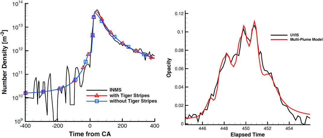
Figure 1. Left: Comparison of the model results with the Cassini INMS E3 Enceladus plume observations. Right: Comparison of the model results with the Cassini UVIS 2007 Enceladus plume observations. The figures are adopted from Tenishev et al. (2014).

The best fit was achieved with a fissure temperature of 180 K and bulk velocities of 350 m/s and 950 m/s for the regular and extra fissures, respectively. These values are consistent with Cassini/CIRS measurements of the surface temperature and the gas thermal velocity (Spencer et al., 2009; Hansen et al., 2011; Goguen et al., 2013). The best fit parameters for the background gas distribution are $c_0=2.7\times 10^{10}$ and $c_1=1.6\times 10^{23}$. The number density due to the background population is at least two orders of magnitude below the peak exospheric density measured by Cassini/INMS. According to our simulations, the column density due to the background population does not exceed 1%–2% at the peak of the column density during UVIS observations. Our findings indicate that Tiger Stripes contribute 23%–32% to the total plume source rate, varying from $6.4\times 10^{27}$ ${\mathrm{s}}^{-1}$ to $29\times 10^{27}$ ${\mathrm{s}}^{-1}$, which is crucial for explaining Cassini/UVIS observations from 2007 to 2010.

4.2 Sodium in the exosphere of the moon

Ground-based observations of the lunar exosphere performed at different phases indicate that sodium number density at the subsolar point is close to $n\approx 60$ ${\mathrm{c}\mathrm{m}}^{-3}$ and varies in altitude with a scale height of 75–120 km (Morgan and Shemansky, 1991; Potter and Morgan, 1988a; Sprague et al., 1992; Sprague et al., 1998; Cremonese and Verani, 1997). At such low densities near the surface, the exosphere is surface-bound. This means that collisions can be neglected in the entire exosphere, and sodium atoms move ballistically, affected only by gravity, solar radiation pressure, and interaction with the surface. Since lunar gravity dominates a neutral particle’s motion in the vicinity of the surface, the initial energy distribution of ejected particles, to a large degree, defines the structure of the exosphere.

Sodium atoms can be released into the exosphere of the Moon through various source processes, with the most significant being thermal desorption, photo-stimulated desorption, sputtering by solar wind, and micrometeorite vaporization (e.g., Morgan and Killen, 1997; Stern, 1999; Morgan and Shemansky, 1991; Sprague, 1992; Smyth and Marconi, 1995; Sarantos et al., 2011; Cintala, 1992).

Micrometeorite vaporization, initially suggested by Potter and Morgan (1988b) as a sodium source in the Moon’s exosphere, has been confirmed by observational studies during meteor stream passages (Hunten et al., 1991; 1998). Numerical modeling by Cintala (1992); Mangano et al. (2007); Sarantos et al. (2008); Lee et al. (2011) investigated its impact on exospheric dynamics. The sodium source rate, ranging from approximately $2\times 10^4$ to $4.9\times 10^4$ atoms ${\mathrm{c}\mathrm{m}}^{-2}$ ${\mathrm{s}}^{-1}$ (Smyth and Marconi, 1995; Morgan and Killen, 1997; Bruno et al., 2006; Bruno et al., 2007), is usually assumed to be uniformly distributed over the lunar surface and fits a Maxwellian distribution with temperatures of 3,000–5000 K (Sarantos et al., 2010; Sarantos et al., 2012b). The deviation from the uniform distribution was investigated by Cremonese et al. (2013), suggesting that the distribution peaks at the equator.

The sputtering of the lunar surface by solar wind and magnetospheric ions significantly contributes to sodium mobilization from the lunar regolith into the exosphere, enhancing sodium atom diffusion from deeper layers for exospheric injection via desorption processes. The sodium flux from sputtering is quantified as ${\mathrm{\Phi }}_s=Y{f}_{\text{Na}}{\mathrm{\Phi }}_i$, where $f_{\text{Na}}=0.0053$ is the surface fraction of sodium, $Y$ is the total sputtering yield, and ${\mathrm{\Phi }}_s$ and ${\mathrm{\Phi }}_{\text{i}}$ are sputtering and incident ion fluxes, respectively (Killen et al., 2007; Mura et al., 2009; Mura et al., 2010; Burger et al., 2010a). The sputtering flux can be reformulated as ${\mathrm{\Phi }}_s={\sigma }_s\sigma {\mathrm{\Phi }}_{\text{i}}$, where $\sigma$ is the surface density of sodium, and ${\sigma }_s$ is a sputtering cross-section. Yakshinskiy and Madey (1999) and Killen et al. (2012) suggest that the surface sodium number density is $\sigma =(3-3.9)\times 10^{12}$ ${\mathrm{c}\mathrm{m}}^{-2}$. Laboratory studies by Dukes et al. (2011) show the cross-section for sputtering of Na on mineral surfaces is ${\sigma }_s=10^{-15}$ ${\mathrm{c}\mathrm{m}}^2$ ${\mathrm{a}\mathrm{t}\mathrm{o}\mathrm{m}\mathrm{s}}^{-1}$, with most sodium sputtered as ions. With a sputtering yield $Y=0.05$ and precipitating flux ${\mathrm{\Phi }}_{\text{SW}}=1-4\times 10^8$ ${\mathrm{c}\mathrm{m}}^{-2}$ ${\mathrm{s}}^{-1}$, the flux of sputtered sodium is about $2.65\times 10^4$ Na ${\mathrm{c}\mathrm{m}}^{-2}$ ${\mathrm{s}}^{-1}$ at the sub-solar point (Wurz et al., 2007; Sarantos et al., 2010; Sarantos et al., 2012b). The energy distribution of sputtered sodium atoms, independent of surface temperature, is given in Equation 22.

$f\left(E_e\right)\sim \frac{E_e}{{\left(E_e+E_b\right)}^3}\left[1-\sqrt{\frac{E_e+E_b}{E_i}{\left(\frac{m_H+m_{\text{Na}}}{4m_H{m}_{\text{Na}}}\right)}^2}\right](22)$

Here, $E_e$ is the ejected energy, $E_b=2$ eV is the binding energy, $E_i$ is the kinetic energy of the incident ion, and $m_H$ and $m_{\text{Na}}$ are the masses of solar wind protons and sodium atoms, respectively (McGrath et al., 1986; Mura et al., 2007; Sarantos et al., 2012a). The exit angle with respect to the local surface normal, $\theta$, follows the Knudsen cosine law $f(\theta )=\cos \theta$ (Cassidy and Johnson, 2005).

Photon stimulated desorption (PSD) has been recognized as a significant sodium source in the Moon’s exosphere, initially suggested by McGrath et al. (1986). The process involves ejecting particles influenced by solar photons, with the total flux of ${\mathrm{\Phi }}_{\text{psd}}=({\mathrm{\Phi }}_{\text{ph}}\cos \psi {\sigma }_{\text{psd}}\sigma )/r_h^2$, where ${\mathrm{\Phi }}_{\text{ph}}=2\times 10^{14}$ photons ${\mathrm{c}\mathrm{m}}^{-2}$ ${\mathrm{s}}^{-1}$ is the flux of solar photons with $h\nu \ge 5$ eV, $\sigma$ is the surface sodium number density, ${\sigma }_{\text{psd}}$ is the cross-section of photon stimulated desorption, $r_h$ is the heliocentric distance, and $\varphi$ is the solar angle (Killen et al., 2012). The typical value of the flux has been evaluated by Sarantos et al. (2012b) to be $2\times 10^6$ atoms ${\mathrm{c}\mathrm{m}}^{-2}$ ${\mathrm{s}}^{-1}$. Yakshinskiy and Madey, (1999), Yakshinskiy and Madey, (2004) discuss the experimental investigations of sodium ejection from lunar samples. The energy distribution of ejected sodium atoms is $f_{\text{psd}}(E)\sim (E{U}^{\beta })/({(E+U)}^{2+\beta })$, where $U=0.052$ eV is characteristic energy related to the surface binding energy and $\beta =0.7$ is a shape parameter (Mouawad et al., 2011; Sprague et al., 2012; Burger et al., 2010b).

Thermal desorption is a mechanism for transferring sodium atoms from the lunar regolith to the exosphere, primarily through the sublimation of adsorbed sodium atoms with the total flux of ${\mathrm{\Phi }}_{\text{td}}=\nu \sigma \exp \left(-U_{\text{td}}/kT\right)$, where $\nu$ is the vibrational frequency of the adsorbed atom with a binding energy of $U_{\text{td}}=0.259$ eV (Stern, 1999; Mura, 2012). The vibrational frequency, typically set at $\nu =10^{13}{\text{s}}^{-1}$ (Killen et al., 2004; Killen et al., 2007; Yakshinskiy et al., 2000; Milillo et al., 2011; Leblanc and Johnson, 2010). The surface temperature, $T$, varies from $300{\cos }^{1/4}\psi +100\text{K}$ on the dayside to $100\text{K}$ on the nightside, where $\psi$ is the subsolar angle (Killen et al., 2012). A more detailed temperature model based on LRO DIVINER data was developed by Hurley et al. (2015).

When a sodium atom collides with the lunar surface, it may be scattered, adsorbed, or chemically bound (Sprague, 1992). Particles that are directly scattered quickly equilibrate to the local surface temperature. The proportion of particles that become adsorbed or bound is governed by the sticking coefficient, which is highly dependent on the local surface temperature (Yakshinskiy and Madey, 2005). Killen et al. (2012) note that only about 50% of these adsorbed particles can be re-emitted into the exosphere through various desorption processes.

The rate of sodium photoionization by solar UV radiation has been a subject of considerable debate. Huebner et al. (1992) provided both theoretical and empirical photoionization rates of $5.92\times 10^{-6}{\text{s}}^{-1}$ and $6.52\times 10^{-6}{\text{s}}^{-1}$ at 1 AU for the quiet and active Sun, respectively, and higher laboratory-derived rates of $1.62\times 10^{-5}{\text{s}}^{-1}$ and $1.72\times 10^{-5}{\text{s}}^{-1}$ for similar conditions. Historically, estimates of sodium photoionization lifetime in the Moon’s exosphere ranged from 12 to 17 h (Potter and Morgan, 1988a; Killen and Ip, 1999; Flynn and Mendillo, 1995; Sprague et al., 1992; Hunten, 1992; Ip, 1991). In more recent work the sodium photoionization lifetime of 36–47 h was assumed (Wilson et al., 1999; Wilson et al., 2003; Line et al., 2012), which is consistent with that by Huebner et al. (1992).

Figure 2 illustrates an example of applying AMPS to model the distribution of sodium in the Moon’s exosphere. Our simulations indicate that photon-stimulated desorption is the dominant source of sodium in the lunar exosphere, with its rate exceeding that of meteoritic impact vaporization by a factor of approximately 8–9. The total source rate of sodium is estimated to be $1.68\times 10^{23}$ atoms per second. Surface interactions play a crucial role in the behavior of sodium atoms, with the majority being reabsorbed by the lunar surface rather than escaping into space. Specifically, about 70% of sodium atoms produced by meteoritic impact vaporization and 25% of those produced by photon-stimulated desorption are reabsorbed, leading to an estimated escape rate from the exosphere of $5.3\times 10^{22}$ atoms per second.

Figure 2

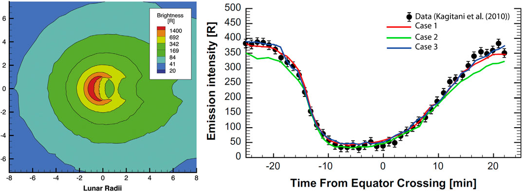
Figure 2. Left: Modeled brightness of the lunar sodium D1 + D2 emission as it would be seen from the Earth on 30 September 1991. Right: Emission of exospheric sodium observed with the UPI-TVIS instrument onboard the SELENE (Kaguya) spacecraft on 7 February 2009 and comparison with the model results. The figure is adapted from Tenishev et al. (2013).

4.3 Kinetic modeling coma of comet 67P/Churyumov-Gerasiminko

Both kinetic and fluid-type methods have been successfully used to model cometary comae. This section illustrates the applications of these methods in studying ESA’s Rosetta mission target, comet 67P/Churyumov-Gerasimenko.

Unlike planets’ dense, collisional atmospheres, cometary comae are characterized by minimal interactions between particles. Cometary comae are a distinctive phenomenon within the solar system, functioning as a planetary atmosphere with minimal influence from gravity. As a comet nears the Sun, water vapor and other gases sublimate, forming a cloud of gas, ice, and refractory materials (such as rocky and organic dust) expelled from the nucleus’s surface. The sublimated gas molecules may experience frequent collisions and participate in photochemical reactions near the nucleus. Due to the comet’s negligible gravity, it generates a large and highly variable dusty coma extending far beyond the cometary nucleus’s size (Hässig et al., 2015).

The sublimation of volatiles from a cometary nucleus is the primary source of volatiles in a cometary coma. The nucleus is covered by a porous layer of ice and solid grains, which experiences periodic solar illumination due to the rotation of the nucleus. This leads to the sublimation of volatiles, thereby contributing to the formation of the coma. Thermal re-radiation, solid-state heat conduction, and mass and energy subsurface transport also play significant roles. These processes collectively form the foundation for the thermophysical modeling of the nucleus’s gas production, which is used to define the boundary conditions on the nucleus’s surface for subsequent modeling of gas dynamics in cometary comae (Davidsson, 2024; Davidsson and Gutiérrez, 2005; Davidsson et al., 2010a).

With a typical density near the surface of $n\approx 10^{19}{\text{m}}^{-3}$ and a water collisional cross-section of $\sigma \approx 10^{-19}{\text{m}}^{-2}$, the mean free path in the coma is $\lambda =\frac{1}{\sqrt{2}n\sigma }<1\text{m}$, which allows for the application of hydrodynamic methods near the nucleus. As the distance from the nucleus increases, the collision rate in the outflowing gas rapidly decreases, making momentum exchange within the gas phase negligible beyond approximately $10^3$ km from the nucleus. Therefore, accurately modeling a cometary coma from the near nucleus region to the far coma requires a kinetic approach, where gas thermalization is described at the level of individual particle collisions. The cross-section values for collisions between major neutral components used in such modeling are summarized in Table 1 based on the works of Crifo (1989) and Combi (1996).

Table 1

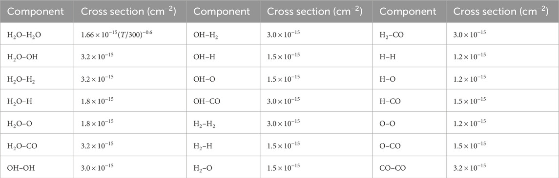
Table 1. Cross sections of collisions for major components of cometary comae.

As the primary species, water dominates the thermodynamic balance of cometary comae through its photodissociation and radiation cooling. Its rotational transitions may allow radiation cooling or heating, which could be essential for controlling ${\text{H}}_2\text{O}$ velocity and temperature in the intermediate and outer coma of active comets (Bockelée-Morvan and Crovisier, 1987; Xie and Mumma, 1996; Marconi and Mendis, 1982). For radiation cooling through the emission of rotational lines to become efficient, the rotational degrees of freedom must be coupled with translational ones. This coupling is possible only when the coma is in the collision-dominated regime. An empirical formula for energy loss by radiation was proposed by Shimizu (1976); Crovisier (1984); Combi (1996).

The evolution of daughter species in the coma primarily depends on the absorption of solar radiation and interaction with the solar wind, which consists mainly of protons, ${\text{He}}^{+}$ ions, and electrons of solar origin. Absorption of solar radiation leads to the excitation of an atom or a molecule, followed by photoionization or photodissociation. Charge exchange and impact ionization due to interaction with the solar wind are the primary channels for the decay of daughter species. The relative density of ions is typically negligible in the collision zone of the coma at moderate to large heliocentric distances. As a result, the effect of ion interactions with neutral species can be neglected when modeling that region.

Starting a few hundred kilometers from the nucleus, the gas dynamics in a cometary coma are primarily influenced by the formation of energetic daughter species (Combi and Smyth, 1988; Xie and Mumma, 1996; Festou, 1999; Gunnarsson et al., 2002). The dominant photolytic process in a coma is the photodissociation reaction ${\text{H}}_2\text{O}+h\nu \to \text{OH}+\text{H}+\mathrm{\Delta }E$, which occurs at a rate of $\beta =1.2\times 10^{-5}{\text{s}}^{-1}$ at a heliocentric distance of 1 AU. This reaction produces a mean energy excess of $\mathrm{\Delta }E=1.78\text{eV}$, corresponding to a mean ejection velocity of $18.5\text{km}{\text{s}}^{-1}$ for H atoms in the rest frame of the parent molecule. Other photodissociation reactions critical in modeling a cometary environment are summarized in Table 2. Photolytic heating, caused by momentum exchange between highly energetic daughter species and other components of the coma, is efficient only in the near-nucleus region, where the dissociation products are thermalized through collisions.

Table 2

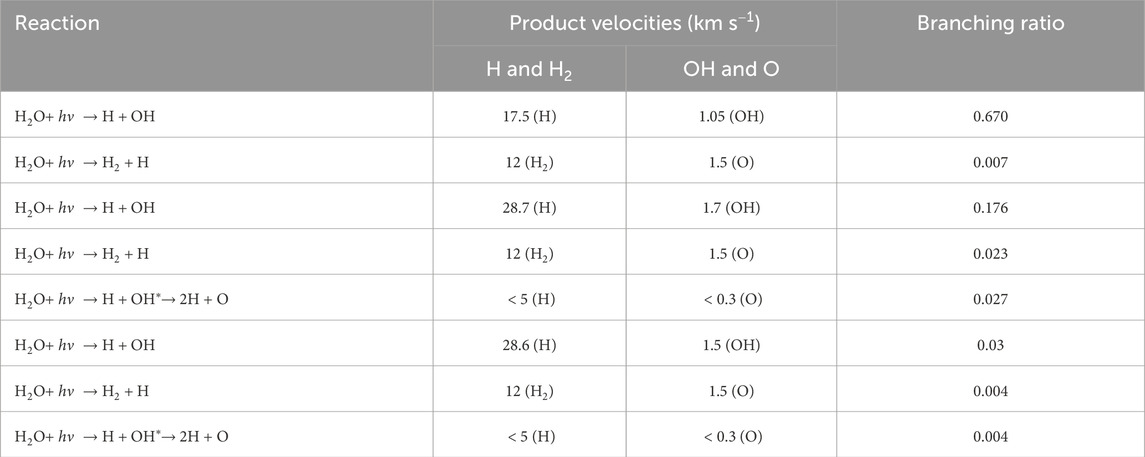
Table 2. Photochemical branching and exothermic velocities for ${\mathrm{H}}_2$O.

The Direct Simulation Monte Carlo (DSMC) method was employed to model the coma of comet 67P/Churyumov-Gerasimenko in both full 3D and axially symmetric 2D, capturing the distribution and dynamics of major volatile species (Combi, 1996; Tenishev et al., 2008). This approach is crucial for understanding the complex interactions within the coma, especially given the non-equilibrium conditions present due to low particle densities and varying illumination conditions. The DSMC model was used to analyze data from the Rosetta Orbiter Spectrometer for Ion and Neutral Analysis (ROSINA) and the Visible and Infrared Thermal Imaging Spectrometer (VIRTIS) onboard the ESA Rosetta mission.

In that modeling, the nucleus was represented with a high-resolution shape model, and the activity was distributed over the surface based on local illumination and empirical data derived from observations (Tenishev et al., 2016). The major species needed to be considered are ${\mathrm{H}}_2$O, ${\mathrm{C}\mathrm{O}}_2$, CO, and ${\mathrm{O}}_2$.

The surface activity can be described using a 25-term (order 4) spherical harmonic expansion, capturing the complex activity patterns observed in different regions of the comet. The coefficients of this expansion were determined through a least-squares optimization method using Rosetta/ROSINA data (Fougere et al., 2016a; Fougere et al., 2016b). The gas flux at the nucleus’ surface was defined by the local surface temperature derived from the thermophysical model of the comet’s nucleus (Davidsson and Gutiérrez, 2004; Davidsson and Gutiérrez, 2006; Davidsson et al., 2010b). The gas flux at the nucleus surface is in Equation 23

$F_k=G\left({\mathrm{\Theta }}_{\text{SZA}}\right)f_k/R_{\text{AU}}^{\beta }(23)$

Here, $G({\mathrm{\Theta }}_{\text{SZA}})$ represents the variation of flux with solar zenith angle (SZA), $f_k$ is the local surface activity factor, and $R_{\text{AU}}$ is the heliocentric distance in astronomical units, and $\beta$ is the exponent corresponding to a power law governing the comet’s source rate evolution with heliocentric distance (Fougere et al., 2016a; Fougere et al., 2016b).

AMPS successfully replicated the temporal and spatial variations observed in the coma of comet 67P/Churyumov-Gerasiminko. It accurately captured the strong seasonal variations in outgassing patterns driven by the comet’s axial tilt. The model demonstrated a strong correlation between water vapor and molecular oxygen throughout the observation period, while ${\mathrm{C}\mathrm{O}}_2$ and CO showed varying correlations pre- and post-equinox. The simulated column densities for ${\mathrm{H}}_2$O and ${\mathrm{C}\mathrm{O}}_2$ matched well with observational data, particularly post-equinox. Some discrepancies were noted, especially for ${\mathrm{C}\mathrm{O}}_2$ densities early in the mission, which could be attributed to the limitations of a single power-law approximation for the extended period.

Figure 3 compares the model with Rosetta’s VIRTIS data, further supporting the model’s accuracy in capturing both the large-scale coma structure and the finer details of local outgassing features.

Figure 3

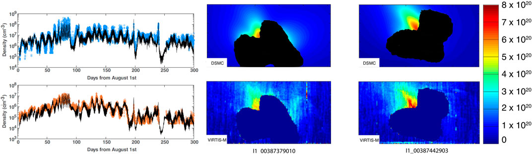
Figure 3. Left: Density extracted at the spacecraft’s location every hour from the DSMC outputs choosing the case from the 48 runs with the closest Sun/comet geometry. The top panel is for water with the DFMS/COPS in blue circles and the DSMC model in black. The bottom panel represents ${\mathrm{C}\mathrm{O}}_2$ with DFMS/COPS data in orange and the DSMC model in black Right: ${\mathrm{H}}_2$O column density (in ${\mathrm{m}}^{-2}$) from the DSMC model (top image of each panel) compared with the corresponding VIRTIS-M observations (bottom image of each panel) from Migliorini et al. (2016) using a linear color scale from 0 to $8\times 10$ ²⁰ ${\mathrm{m}}^{-2}$. The figure is adapted from Fougere et al. (2016b).

4.3.1 Hydrodynamic methods for modeling volatiles in a cometary coma

Even when the inner coma comprises a large fluid region, a Knudsen layer, where gas released from the nucleus becomes thermalized, inevitably separates it from the nucleus. Therefore, to apply a hydrodynamic approach to a cometary coma, boundary conditions must be set not on the nucleus’s surface but at the top of the Knudsen layer. Studies highlight that the thickness of the Knudsen layer typically ranges from a few meters to several hundred meters (Crifo, 1987; 1989; Rickman, 1989; Crifo et al., 2002).

The multi-fluid model BATSRUS was used to model neutral gas in the coma of comet 67P/Churyumov-Gerasiminko. The relevant methodology is discussed in Section 3.2. The model includes multiple gas species, such as ${\mathrm{H}}_2$O, CO, and ${\mathrm{C}\mathrm{O}}_2$, and their dissociation products. Each is treated as a distinct fluid with unique density, velocity, and temperature. The initial and boundary conditions are derived from a thermophysical model of the comet nucleus, which provides gas flux and temperature.

In comparing the multi-fluid model with the DSMC approach for modeling gas dynamics in a cometary coma, the multi-fluid model can achieve results generally consistent with those obtained from the DSMC method. Despite the inherent approximations and simplifications in the multi-fluid approach, such as treating each gas species as a separate fluid with its density, velocity, and temperature, the model effectively captures the critical physical processes, including photochemical reactions and collisional dynamics. The multi-fluid model’s ability to reproduce the general trends in gas density, velocity, and temperature profiles, as observed in the DSMC simulations, confirms its validity and accuracy on large spatial scales up to $10^6$ km.

Comparison illustrated in Figures 4, 5 indicates that the gas velocity and density are consistent with a kinetic model. However, higher moments, such as temperature, are not fully reproduced as the kinetic nature of particle interactions determines their dynamics. As illustrated in Figure 6, the temperatures of daughter species are accurately reproduced in the inner coma, where particle collisions still maintain thermodynamic equilibrium, while an increase in the primary species’ temperature, specifically ${\mathrm{H}}_2$O, at distances of $10^6-10^7$ km was not captured by the model.

Figure 4

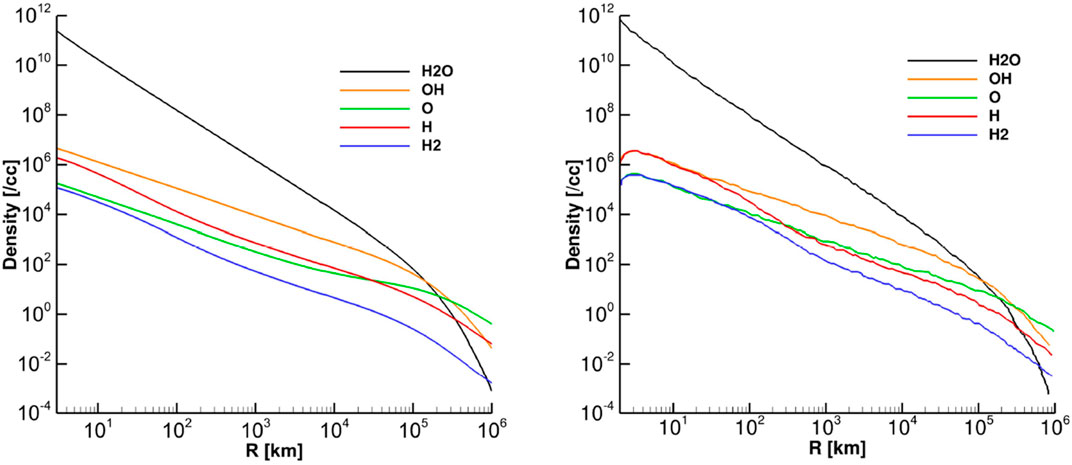
Figure 4. Densities of modeled species vs. distances from the body for a heliocentric distance of 1.3 au and a production rate of $5\times 10$ ²⁷ ${\mathrm{s}}^{-1}$, respectively. The left column shows our fluid model results and the right column shows the results reproduced from Tenishev et al. (2008). This figure has been adapted from Shou et al. (2016).

Figure 5

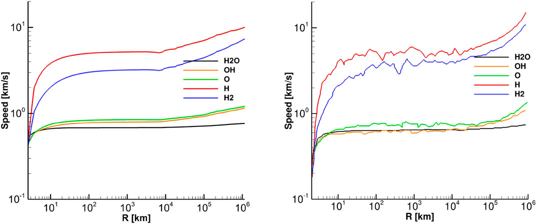
Figure 5. Speed of modeled species vs. distances from the body for a heliocentric distance of 1.3 au and a production rate of $5\times 10$²⁷ ${\mathrm{s}}^{-1}$, respectively. The left column shows our fluid model results and the right column shows the results reproduced from Tenishev et al. (2008). This figure has been adapted from Shou et al. (2016).

Figure 6

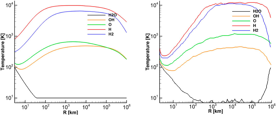
Figure 6. Temperatures of modeled species vs. distances from the body for a heliocentric distance of 1.3 au and a production rate of $5\times 10$ ²⁷ ${\mathrm{s}}^{-1}$, respectively. The left column shows our fluid model results and the right column shows the results reproduced from Tenishev et al. (2008). This figure has been adapted from Shou et al. (2016).

This temperature increase is a kinetic effect caused by ${\mathrm{H}}_2$O collisions with energetic secondary species in the innermost coma, where the density is still high enough for collisions. These collisions create a minor high-energy population of ${\mathrm{H}}_2$O, which does not significantly affect the bulk velocity or temperature in the innermost coma. However, the effect of photoionization and photo-dissociation of the primary species results in the removal of predominantly slower-moving molecules from the population. This makes the high-energy ${\mathrm{H}}_2$O population more pronounced, increasing the overall kinetic temperature, as seen in Figure 6.

4.3.2 A dusty gas flow in a cometary coma

Dust and gas are the primary components of a cometary coma, with dust being entrained by sublimating gas. Ground-based observations of dust rely on scattered light (Harris et al., 1997; Sarmecanic et al., 1997; Harmon et al., 1997; Jewitt and Matthews, 1997; Moreno, 2009). Recent observations of dust in the coma of comet Churyumov-Gerasimenko with ESA Rosetta’s OSIRIS and VIRTIS provided unprecedented observations of cometary dust (e.g.,. Agarwal et al., 2009; Agarwal et al., 2010; Agarwal et al., 2016; Lara et al., 2015; Lin et al., 2015; Schultz et al., 2010).

The widely accepted view is that sunlight heating is the primary factor determining gas and dust ejection rates from a comet’s nucleus, making these rates dependent on the sub-solar angle (Tenishev et al., 2008; Belton, 2013). It is also generally assumed that the dust ejection rate is proportional to that of gas (Tenishev et al., 2011). However, Clark et al. (2004) suggested that other factors, such as thermal stress or internal gas pressure, might also contribute to dust release. The sunset jet observed by OSIRIS on Rosetta suggests that a thermal lag in the nucleus’s upper subsurface layer may play a significant role Shi et al. (2016).

Dust particles observed by Rosetta are categorized into two main types: compact particles, with diameters between 0.03 and 1 mm, and fluffy particles, with diameters ranging from 0.2 to 2.5 mm (Della Corte et al., 2015; Rotundi et al., 2015). Despite their larger size, fluffy particles contribute minimally to the overall dust mass ejection rate (Fulle et al., 2019; Fulle et al., 2017; Fulle et al., 2015; Fulle and Blum, 2017). The formation of fluffy particles has been investigated by Skorov and Blum (2012). Additionally, smaller particles, known as nanograins, were detected by the Ion and Electron Sensor onboard Rosetta at 50–65 km from the comet (Burch et al., 2015). Most compact particles observed by the Grain Impact Analyser and Dust Accumulator experiment onboard Rosetta have masses ranging from $7.5\times 10^{-8}$ to $1.6\times 10^{-7}$ kg, traveling at velocities of 1–6 m/s (Torre et al., 2015). Analysis of dust particles collected by Rosetta/COSIMA revealed no evidence of volatiles being carried by these particles (Schulz et al., 2015).

Based on spectral energy distribution (SED) observations, Sekanina and Farrell (1982) derived a grain size distribution given by $n(a)=g_1{(1-a/a_0)}^M{(a/a_0)}^N$, which fits the SEDs of several comets (Hanner et al., 1985; Hanner and Campins, 1986; Sekanina et al., 2001; Divine et al., 1986). In this model, $g_1$ is a normalization factor, $a_0=0.1\mu m$ is the minimum grain radius, $N$ (approximately 3.7–4.2) defines the slope for large grain radii, and $M$ (approximately 2–8) determines the grain radius $a_P=a_0(M+N)/N$ where the distribution peaks. A simpler grain size distribution, $f(a)\sim a^s$, has also been proposed (Hanner, 1982; Divine et al., 1986; Grün et al., 1989), where $s$ is a power index.

For comet 67P/Churyumov-Gerasimenko, the dust size distribution’s power index ranges from $-4.1$ to $-3.5$ (Agarwal et al., 2010; Fulle et al., 2010; Ishiguro, 2008; Ishiguro et al., 2009; Kelley et al., 2008; Kelley et al., 2009; Marschall et al., 2020). Rotundi et al. (2015) reported a dust-to-gas mass ratio of $4\pm 2$, a differential size distribution power index of $-4$, and a dust-loss rate of $7\pm 1{\text{\hspace{0.17em}kg\hspace{0.17em}s}}^{-1}$ at heliocentric distances of 3.4–3.6 au.

The motion of dust particles near the nucleus is primarily governed by the combined effects of gas drag and gravity forces (Equation 24).

$\frac{d{v}_g}{dt}=\frac{1}{m_g}\left[\pi a^2\frac{C_D}{2}\rho \left(v-v_g\right)|v-v_g|-F_g\right](24)$

Here, $m_g=\frac{4}{3}\pi a^3{\rho }_g$ represents the mass of a spherical dust particle, $C_D$ is the drag coefficient, $F_g$ is the gravitational force acting on the particle, $v$ is the bulk velocity of the ambient gas in the coma, $v_g$ is the velocity of a dust particle with radius $a$, and $\rho$ and ${\rho }_g$ are the mass densities of the ambient gas and dust particles, respectively. A more comprehensive analysis of dust particle trajectories in the coma of comet 67P/Churyumov–Gerasimenko, accounting for nucleus rotation, was conducted by Kramer and Noack (2016). The consideration of non-spherical particles in dust transport modeling is discussed by Fulle and Blum (2017).

Assuming a spherical shape for the dust grain, a common approach in the comet community, the drag coefficient $C_D$ is typically determined for conditions of a free molecular flow, isothermal dust grains, and diffuse reflection of gas molecules (Equation 25).

$C_D=\frac{2s^2+1}{s^3\sqrt{\pi }}\exp \left(-s^2\right)+\frac{4s^4+4s^2-1}{2s^4}\text{erf}\left(s\right)+\frac{2\sqrt{\pi }}{3s}\sqrt{\frac{T_d}{T_g}},(25)$

Here, $s=|v_g-v_d|/\sqrt{2k_B{T}_g/m_g}$, and $T_d$ and $T_g$ are the temperatures of the dust grain and the ambient gas, respectively (e.g., Crifo et al., 2005). For practical calculations, the drag coefficient is often approximated as a constant $C_D=2$, which adequately represents the gas-dust interaction under typical conditions in cometary comae (Tenishev et al., 2011; Della Corte et al., 2015; Gombosi et al., 1986; Grün et al., 1989; Tenishev et al., 2016) Alternative approximations of the drag coefficient $C_D$ have been presented by Rodionov et al. (2002), Baines et al. (1965), and Nakamura et al. (1994).

Remote sensing observations of dust in a cometary coma rely on measuring its brightness. The optical properties of dust grains, derived from these observations, are detailed by Kolokolova et al. (2004); Lasue et al. (2009); Shen et al. (2009), where dust brightness is obtained by taking the following integral:

$I\left(\lambda \right)=F\left(\lambda \right)\int n\left(r\right){\sigma }_g{q}_s\left(\lambda \right)\frac{p\left(g\right)}{4\pi }ds,(26)$

where $F(\lambda )$ is the solar flux at a comet’s location, $n(r)$ is a dust number density, ${\sigma }_g$ is the geometrical cross-section of a dust grain, $q(\lambda )$ is a scattering efficiency, and $p(g)$ is a normalized phase function (e.g., Kolokolova et al., 2004; Fink and Rubin, 2012; Fink and Rinaldi, 2015; Tenishev et al., 2016).

Figure 7 presents the results of the analysis of the dust jet observed by Rosetta/VIRTIS-M on 12 April 2015 (2015-04–12T07:14:00) (Migliorini et al., 2016). We calculated the dust brightness as Rosetta would see using the simulated cometary dust distribution and compared it with the coma brightness observed by Rosetta/VIRTIS-M.

Figure 7

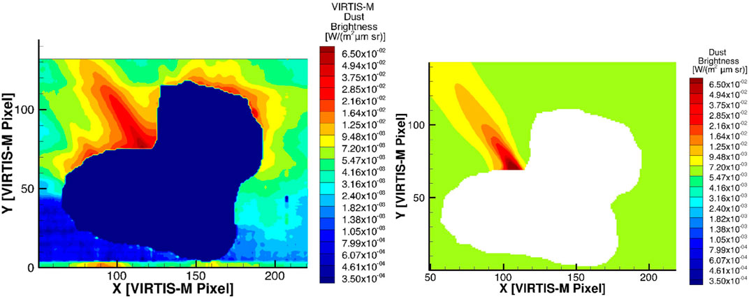
Figure 7. Comparison of the cometary dust brightness map observed by Rosetta/VIRTIS-M [observation I1˙00387442903 taken on 2015-04-12T07:14:00, Migliorini et al. (2016)] with that from our kinetic modeling of gas and dust in the coma of comet 67P/Churyumov–Gerasimenko. The observed brightness map is shown in the left panel, and the modeled map is in the right panel. The X- and Y-axes represent the instrument’s pixel grid. The figure is adapted from Tenishev et al. (2016).

Following the calibration procedure established by the Rosetta/VIRTIS team, we assumed a solar flux of $F(1.09\mu \text{m})=586.86{\text{W\hspace{0.17em}m}}^{-2}\mu {\text{m}}^{-1}$ at one au. On 12 April 2015, when the comet was at a heliocentric distance of 1.88 au, this flux scaled to $F(1.09\mu \text{m}){|}_{1.88\text{au}}=166{\text{W\hspace{0.17em}m}}^{-2}\mu {\text{m}}^{-1}$, which we used for calculating the dust brightness as defined in Equation 26. Scattering efficiency, $q_s(\lambda )$, was calculated assuming ‘Halley-dust’ particles with the ice-to-dust ratio of 0.05, and porosity of 0.83 (Nagdimunov et al., 2014). We adopted a dust mass density of $\rho =1000{\text{kg\hspace{0.17em}m}}^{-3}$ and experimented with a power-law index for the dust size distribution, finding that a value of $-2.5$ provided the best match to the observed images, consistent with the findings of Marschall et al. (2016) for Rosetta/OSIRIS dust images. The simulated dust particle radii ranged from $10^{-7}$ to $10^{-3}$ m. We estimate that the dust source region covered about 1.3% of the total nucleus surface area. With a total dust-to-gas ratio of six and a gas production rate from Fougere et al. (2016b), the total dust mass source rate was approximately 71 kg ${\mathrm{s}}^{-1}$, with 2.6% of the dust ejected into the jet.

4.4 Mars’ hot oxygen corona

Mars’ hot oxygen corona, first predicted by McElroy (1972) as a result of dissociative recombination of ionospheric ${\mathrm{O}}_2^{+}$ with electrons in the exosphere, was confirmed by Rosetta/ALICE during its 2007 Mars flyby. The spacecraft detected the atomic oxygen resonance line at 130.4 nm, providing direct evidence of the corona’s existence (Feldman et al., 2011; Gröller et al., 2014).

Later, the MAVEN mission provided detailed observations of Mars’ upper atmosphere (Deighan et al., 2015). While direct escape rate measurements are not feasible (Leblanc et al., 2017), MAVEN’s instruments have allowed indirect estimates of hot oxygen density and escape rates, ranging from 1.2 to $5.5\times 10^{25}{\text{s}}^{-1}$, depending on season and solar activity (Jakosky et al., 2015; Lillis et al., 2017). Additionally, MAVEN’s Imaging Ultraviolet Spectrograph (IUVS) has systematically observed 130.4 nm coronal emissions since 2014, revealing exobase densities from $6.3\times 10^3$ to $8.0\times 10^3{\mathrm{c}\mathrm{m}}^{-3}$ during low solar activity and up to $1.2\times 10^4{\mathrm{c}\mathrm{m}}^{-3}$ during moderate activity, with effective temperatures between 4,100 and 4500 K (Chaufray et al., 2015; Deighan et al., 2015; McClintock et al., 2015; Qin et al., 2024).

Mars experiences significant atmospheric loss, primarily of hydrogen and oxygen, with total escape rates ranging from 2 to 3 kg/s, primarily from water and carbon dioxide. Oxygen loss occurs through several processes: solar wind-driven electric field acceleration, which removes oxygen ions at a rate of $5\times 10^{24}$ atoms per second (130 g/s); photochemical processes, particularly dissociative recombination, which contribute a neutral oxygen loss rate of $5\times 10^{25}$ atoms per second (1,300 g/s); and sputtering caused by solar wind ions, leading to an additional loss of $3\times 10^{24}$ oxygen atoms per second (80 g/s) (Jakosky et al., 2018).

Space weather significantly affects hot oxygen production in Mars’ upper atmosphere. For example, the X8.2-class solar flare on 10 September 2017, increased hot oxygen production by up to 45% and photochemical escape rates by 20% due to enhanced ultraviolet flux (Fox, 2004; Fox and Hac, 2009; Lee et al., 2018; Cravens et al., 2017).

Both empirical and physics-based modeling are used to analyze MAVEN’s data. Such, Ramstad et al. (2023) developed an empirical method using MAVEN’s in situ measurements to infer Mars’ hot oxygen density near the exobase, finding densities of $6\text{–}7\times 10^3{\text{cm}}^{-3}$ and effective temperatures of $3700\text{–}3800\text{K}$. Various physics-based models were developed to investigate the production mechanisms and distribution of those energetic atoms (e.g., Chaufray et al., 2007; Fox and Hac, 2009; Gröller et al., 2014; Hodges, 2000; Lee et al., 2015a; b; Lee, 2014; Valeille, 2009; Valeille et al., 2010).

The most commonly used numerical method for analyzing MAVEN/IUVS observations of Mars’ hot oxygen corona is Monte Carlo modeling, which simulates the transport of hot oxygen from its production in the thermosphere through the exosphere and into the corona to compare with observations (Leblanc et al., 2017; Lee et al., 2015a).

As hot oxygen (O) atoms propagate through the thermosphere, they may collide with ambient atoms and molecules, losing energy and becoming thermalized before reaching the corona. However, collisions between a hot O atom and a thermal O atom in the thermosphere can energize the latter enough to enter the corona. The energy transferred during collisions highly depends on the total and angular differential scattering cross-sections. Forward scattering is crucial in modeling this process because it affects how hot O atoms retain energy after collisions with ${\mathrm{C}\mathrm{O}}_2$, reducing thermalization and allowing more hot O atoms to escape Mars’ gravity. Accurate forward scattering modeling is essential for estimating the density of the hot O corona and photochemical loss rates, which are critical for understanding Mars’ atmospheric evolution (Gacesa et al., 2020; Fox and Hać, 2014; Gacesa et al., 2017; Lee et al., 2020; Kharchenko et al., 2000; Valeille, 2009; Valeille et al., 2009b).

The results of modeling the hot O population in Mars’ corona using AMPS are illustrated in Figure 8. The simulation was initialized using outputs from the Mars Global Ionosphere Thermosphere Model (M-GITM) (Bougher et al., 2014), which provides a detailed description of the background thermosphere, including temperature, wind, and density profiles of significant species such as O, ${\mathrm{C}\mathrm{O}}_2$, and ${\mathrm{N}}_2$. M-GITM accounts for diurnal, seasonal, and solar cycle variations, ensuring that the initial conditions accurately reflect the current Martian atmospheric state.

Figure 8

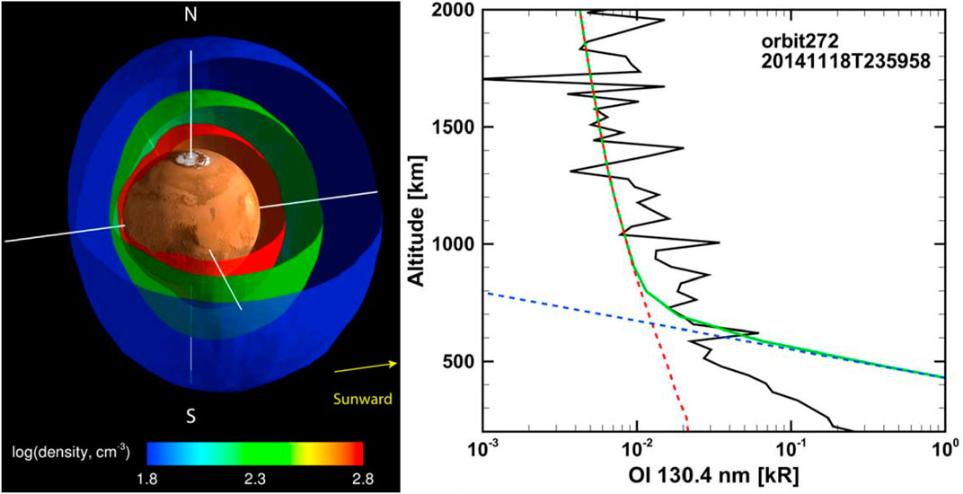
Figure 8. Left: Three-dimensional representation of the Martian hot corona. Three isodensity surfaces of hot atomic oxygen are shown, decreasing with increasing distance from the planet: red, 600 ${\mathrm{c}\mathrm{m}}^{-3}$; green, 200 ${\mathrm{c}\mathrm{m}}^{-3}$; blue, 60 ${\mathrm{c}\mathrm{m}}^{-3}$. The north and south pole positions are indicated by their initials N and S, respectively. The yellow arrow points toward the Sun. The figure is adapted from Valeille et al. (2009b). Right: Comparisons of the modeled OI 130.4 nm brightness from the simulation by the period M-GITM coupled framework with the IUVS/MAVEN coronal limb scan data for a selected set of orbits during a period from 12 November 2014, to 17 January 2015, (Deighan et al., 2015). The black solid curves indicate the IUVS observations. The model prediction of total exospheric O brightness is shown by the green solid curves, decomposed into the hot (red dash) and cold (blue dash) components in each plot. The estimated transition altitude by the model is approximately where the blue and red curves are crossed. The figure is adapted from Lee et al. (2015b).

Below the exobase, the atmosphere is assumed to be in collisional equilibrium with a Maxwellian velocity distribution. This approach was used to model the transport of hot O atoms through the thermosphere, where they originated and interacted with the background population of major thermospheric species. The simulation incorporated key model parameters, including the distribution of hot O source strength and the density of background species, derived from M-GITM outputs for specific solar cycle and seasonal conditions, ensuring that the thermospheric state was accurately represented.

Energy-dependent forward scattering cross-sections for O-O and O-${\mathrm{C}\mathrm{O}}_2$ interactions from Kharchenko et al. (2000) were used in the modeling. The escape energy for oxygen atoms was set at 1.97 eV, corresponding to the gravitational potential energy required to overcome Mars’ gravity. To ensure statistical convergence and accurate representation of the hot oxygen population, the simulation utilized a large number of particles, typically on the order of $10^6$ to $10^7$. The effect of producing secondary hot O is discussed in previous studies (e.g., Lee et al., 2015b; Lee et al., 2018; Lee et al., 2020).

The parameters for the dissociative recombination reaction used in this study are summarized in Table 3. The reaction rate constant, as detailed in Equation 27, is adapted from Mehr and Biondi (1969) and has been employed in our previous research on Mars’ hot oxygen corona (e.g., Lee et al., 2015b; Valeille et al., 2010).

$\alpha =\left\{\begin{array}{cc}1.95\times 10^{-7}{\left(\frac{300}{T_e}\right)}^{0.7}{\mathrm{c}\mathrm{m}}^3{\mathrm{s}}^{-1},\hfill & 300<T_e<1200\mathrm{K}\hfill \\ 7.39\times 10^{-8}{\left(\frac{1200}{Te}\right)}^{0.56}{\mathrm{c}\mathrm{m}}^3{\mathrm{s}}^{-1},\hfill & 1200<T_e<5000\mathrm{K}\hfill \end{array}\right.(27)$

Table 3

Table 3. ${\mathrm{O}}_2^{+}$ dissociative recombination channels, excess energies, and branching rations.

The Martian hot oxygen corona simulation using the AMPS model, cuand ITM, rvealed that the hot oxygen population is highly variable and strongly influenced by both solar cycle and seasonal changes. The study found that solar maximum periods produce significantly higher densities and escape rates of hot oxygen, with global escape rates ranging from $1.14\times 10^{25}{\mathrm{s}}^{-1}$ during solar minimum to $5.18\times 10^{25}{\mathrm{s}}^{-1}$ during solar maximum (Lee, 2014). Seasonal variations were also prominent, with increased densities observed during perihelion due to the associated changes in thermospheric conditions (Lee et al., 2015b).

4.5 Venus hot oxygen corona and exosphere

Venus’s thermosphere, ionosphere, and exosphere have been extensively studied over several decades through observations from a range of spacecraft missions. These investigations began during the Soviet Venera and US Mariner missions, continued through the nearly 14-year Pioneer Venus mission, and have extended into more recent times with the Venus Express mission (Bougher et al., 1997; Schubert et al., 2007; Gérard et al., 2017).

Most of our current knowledge of Venus’ upper atmosphere and corona comes from measurements made by in-situ and remote sensing experiments on the Pioneer Venus Orbiter (PVO) from December 1978 to October 1992. The “hot” O corona was observed with an ultraviolet spectrometer (UVS) onboard PVO by measuring the OI resonance triplet near 1304 Å (Nagy et al., 1981).

Since 2006, systematic monitoring by Venus Express (VEx) instruments has enhanced our understanding of Venus’s atmosphere. VIRTIS observations have measured 3D temperatures and derived thermal wind fields at 40–90 km (Piccialli et al., 2012; Piccialli et al., 2008) and mapped the highly variable ${\mathrm{O}}_2$ IR nightglow distribution (Drossart et al., 2007; Gérard et al., 2008; Gérard et al., 2009; Gérard et al., 2017; Hueso et al., 2008; Piccioni et al., 2009; Soret et al., 2012; Soret et al., 2014) to trace winds at 90–130 km. SPICAV’s airglow observations of NO emissions (Collet et al., 2010; Gérard et al., 2008; Gérard et al., 2009; Stiepen et al., 2013) and vertical profiles of atmospheric density (Bertaux et al., 2007) have confirmed patterns observed with previous missions (Stewart et al., 1980). These VEx datasets provide critical insights into Venusian atmospheric processes (Brecht et al., 2011).

The BepiColombo spacecraft’s second fly-by of Venus on 10 August 2021, using the Mass Spectrum Analyzer (MSA) on Mio, BepiColombo’s magnetospheric orbiter, revealed cold oxygen (${\mathrm{O}}^{+}$) and carbon (${\mathrm{C}}^{+}$) ions at six planetary radii with a flux of $4\pm 1\times 10^4{\text{cm}}^{-2}{\text{s}}^{-1}$. The ${\mathrm{C}}^{+}$ to ${\mathrm{O}}^{+}$ ion ratio, at most $0.31\pm 0.2$, suggests contributions from CO or water group ions as oxygen sources. These findings, observed near the magnetic pileup boundary, have significant implications for understanding Venus’s atmospheric evolution and the planet’s water history, offering insights into the climate and habitability of terrestrial planets and exoplanetary systems (Hadid et al., 2024).

In the upper atmosphere of Venus, suprathermal O atoms are primarily produced by exothermic reactions, such as the electron dissociative recombination of ${\mathrm{O}}_2^{+}$ ions, similar to the processes observed on Mars (Krestyanikova and Shematovich, 2006; Lichtenegger et al., 2006; Gröller et al., 2010; Gröller et al., 2012; Kella et al., 1997). Unlike the lower thermosphere, where these hot atoms are rapidly thermalized by frequent collisions, in the upper thermosphere and exosphere, where collisions are rare, these hot atoms remain unthermalized, forming extended coronae of H and O atoms above the exobase, located near 200 km. Early estimates of “hot” O density derived from PVO/UVS data suggested a significant population, but later observations did not confirm these findings. Instruments such as SPICAV and ASPERA-4 on board Venus Express, which were sensitive enough to detect “hot” O if present at densities similar to those suggested by PVO data, have not detected this population above their detection thresholds (Bertaux et al., 2007; Galli et al., 2008; Lichtenegger et al., 2009). Despite this, earlier studies using data from the PVO/UVS instrument and the Venera 11 mission had established the presence of a corona of hot O atoms, with densities around $10^4{\text{cm}}^{-3}$ at altitudes of 1000 km (Nagy et al., 1981; Nagy and Cravens, 1988; Bertaux et al., 1981).

The Mars oxygen corona model detailed in Section 4.4 was modified to study Venus’s exosphere and corona (Tenishev et al., 2022). This adaptation takes advantage of the fact that the production and dynamics of hot oxygen on Mars and Venus are similar (Valeille et al., 2009b; Valeille et al., 2009a; Lee et al., 2015a). Similarly, we use the output of the Venus Thermosphere General Circulation Model (VTGCM) of Venus’ thermosphere/ionosphere composition to determine the source of hot O and characterize its interaction with major thermospheric species (Bougher et al., 1988).

Our findings indicate that the altitude distribution of hot oxygen during solar maximum aligns closely with observations from the Pioneer Venus Orbiter. Conversely, during solar minimum, we observe a significant decrease in the oxygen density of the corona, consistent with Venus Express’s non-detection of the oxygen corona. The conditions during moderate solar activity naturally lie between these extremes. Our results indicate variability in the density of the extended oxygen corona around Venus by a factor of six over a solar cycle, aligning with observations suggesting a significant reduction in density during low solar activity periods (Gérard et al., 2017). The lack of corona detection by ASPERA-4 and SPICAV onboard Venus Express during solar minimum further supports our findings, highlighting the effect of solar conditions on the visibility of Venus’ oxygen corona (Lichtenegger et al., 2009). The modeling results of Venus’s exosphere and corona are in Figure 9.

Figure 9

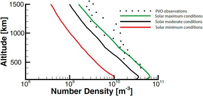
Figure 9. The simulated altitude variation of the energetic hot oxygen population is depicted in the figure. The lines represent model results for solar minimum, moderate, and maximum conditions. The points indicate the altitude variation from the Pioneer Venus Orbiter’s measurement of Venus’ oxygen corona Paxton and Meier (1986). This figure has been adapted from Tenishev et al. (2022).

5 Conclusion

This paper provides an extensive overview of the methods and models used to study exospheres, highlighting analytical and numerical approaches. Foundational analytical models, such as the Chamberlain and Haser models, have proven invaluable tools for the initial analysis of density distributions within exospheres and cometary comae.

The numerical methods, particularly the Direct Simulation Monte Carlo (DSMC) method, and tools like the Adaptive Mesh Particle Simulator (AMPS) have significantly advanced our ability to simulate complex, non-equilibrium gas flows in exospheres. These methods capture a wide range of physical processes, including particle collisions, chemical reactions, and surface interactions, which are critical for accurately modeling the behavior of gases in the tenuous atmospheres of planets, moons, and cometary comae. The multi-fluid model BATSRUS has enhanced our capability to model neutral gases in cometary comae by treating different gas species as distinct fluids. The paper’s case studies, including the Enceladus plume, the Moon’s sodium exosphere, the coma of comet 67P/Churyumov-Gerasimenko, and the hot oxygen coronae of Mars and Venus, illustrate the practical application and effectiveness of these models.

Data availability statement

The original contributions presented in the study are included in the article/supplementary material, further inquiries can be directed to the corresponding author.

Author contributions

VT: Conceptualization, Investigation, Software, Writing–original draft, Writing–review and editing. YS: Software, Writing–review and editing. YL: Software, Writing–review and editing. YM: Writing–review and editing. MC: Writing–review and editing.

Funding

The author(s) declare that financial support was received for the research, authorship, and/or publication of this article. The authors acknowledges the support of the Heliophysics and Planetary Science Branch of Marshall Space Flight Center.

Conflict of interest

The authors declare that the research was conducted in the absence of any commercial or financial relationships that could be construed as a potential conflict of interest.

Publisher’s note

All claims expressed in this article are solely those of the authors and do not necessarily represent those of their affiliated organizations, or those of the publisher, the editors and the reviewers. Any product that may be evaluated in this article, or claim that may be made by its manufacturer, is not guaranteed or endorsed by the publisher.

References

Abe, T. (1993). Generalized scheme of the no-time-counter scheme for the DSMC in rarefied gas flow analysis. Comput. and Fluids 22, 253–257. doi:10.1016/0045-7930(93)90057-g0045-7930(93)90057-G

CrossRef Full Text | Google Scholar

Agarwal, J., A’Hearn, M. F., Vincent, J.-B., Güttler, C., Höfner, S., Sierks, H., et al. (2016). Acceleration of individual, decimetre-sized aggregates in the lower coma of comet 67P/Churyumov-Gerasimenko. Mon. Notices R. Astronomical Soc. 462, S78–S88. doi:10.1093/mnras/stw2179

CrossRef Full Text | Google Scholar

Agarwal, J., Müller, M., and Grün, E. (2009). “Dust environment modelling of comet 67p/churyumov-gerasimenko,” in Rosetta. ESA’s mission to the origin of the solar system. Editors R. Schulz, C. Alexander, H. Boehnhardt, and K. H. Glassmeier (Springer), 99–131.

CrossRef Full Text | Google Scholar

Agarwal, J., Müller, M., Reach, W. T., Sykes, M. V., Boehnhardt, H., and Grün, E. (2010). The dust trail of comet 67p/churyumov-gerasimenko between 2004 and 2006. Icarus 207, 992–1012. doi:10.1016/j.icarus.2010.01.003

CrossRef Full Text | Google Scholar

Babovsky, H., and Illner, R. (1989). A convergence proof for Nanbu’s simulation method for the full Boltzmann equation. SIAM J. Numer. Analysis 26, 45–65. doi:10.1137/0726004

CrossRef Full Text | Google Scholar

Baines, M. J., Williams, I. P., Asebiomo, A. S., and Agacy, R. L. (1965). Resistance to the motion of a small sphere moving through a gas. Mon. Notices R. Astronomical Soc. 130, 63–74. doi:10.1093/mnras/130.1.63

CrossRef Full Text | Google Scholar

Belton, M. J. (2013). The sources of the unusual dust jets seen in comet 103P/Hartley 2. Icarus 222, 653–661. doi:10.1016/j.icarus.2012.12.007

CrossRef Full Text | Google Scholar

Bertaux, J. L., Blamont, J. E., Kurt, V. M., Romanova, N. N., and Smirnov, S. (1981). Venera 11 and venera 12 observations of e.u.v. emissions from the upper atmosphere of venus. Planet. Space Sci. 29, 149–164. doi:10.1016/0032-0633(81)90029-5

CrossRef Full Text | Google Scholar

Bertaux, J.-L., Vandaele, A.-C., Korablev, O., Villard, E., Fedorova, A., Fussen, D., et al. (2007). A warm layer in Venus’ cryosphere and high-altitude measurements of (hf), (hcl), (h)₂(o) and (hdo). Nature 450, 646–649. doi:10.1038/nature05974

PubMed Abstract | CrossRef Full Text | Google Scholar

Bird, G. (1970). SYNOPTIC: breakdown of translational and rotational equilibrium in gaseous expansions. AIAA J. 8, 1997. doi:10.2514/3.49883

CrossRef Full Text | Google Scholar

Bird, G. (1994). Molecular gas dynamics and the direct simulation of gas flows. Oxford University Press.

Google Scholar

Bockelée-Morvan, D., and Crovisier, J. (1987). “The role of water in the thermal balance of the coma,” in Proceedings of the international symposium on the diversity and similarity of comets (Paris: European Space Agency), 235–240.

Google Scholar

Borgnakke, C., and Larsen, P. S. (1975). Statistical collision model for Monte Carlo simulation of polyatomic gas mixture. J. Comput. Phys. 18, 405–420. doi:10.1016/0021-9991(75)90094-7

CrossRef Full Text | Google Scholar

Bougher, S., Dickinson, R., Ridley, E., and Roble, R. (1988). Venus mesosphere and thermosphere. Icarus 73, 545–573. doi:10.1016/0019-1035(88)90064-4

CrossRef Full Text | Google Scholar

Bougher, S. W., Alexander, M. J., and Mayr, H. G. (1997). “Venus II: geology, geophysics, atmosphere, and solar wind environment hunten, and R.J. Philips,” in Upper atmosphere dynamics: global circulation and gravity waves (Tucson, AZ: University of Arizona Press), 259. chap.

Google Scholar

Bougher, S. W., Combi, M., Lee, Y., Tenishev, V., and Dong, C. (2014). “Hot O corona in Mars upper atmosphere: solar cycle and seasonal variations and implications for neutral and ion escape rates,” in 6th alfven conference.

Google Scholar

Boyd, I. D. (1991). Analysis of vibrational-translational energy transfer using the direct simulation Monte Carlo method. Phys. Fluids A 3, 1785–1791. doi:10.1063/1.857959

CrossRef Full Text | Google Scholar

Boyd, I. D. (1996). A threshold line dissociation model for the direct simulation Monte Carlo method. Phys. Fluids 8, 1293–1300. doi:10.1063/1.868899

CrossRef Full Text | Google Scholar

Boyd, I. D. (1999). Nonequilibrium chemistry modeling in rarefied hypersonic flows. AIAA-1999-3634.

CrossRef Full Text | Google Scholar

Boyd, I. D., Bose, D., and Candler, G. V. (1997a). Monte Carlo modeling of nitric oxide formation based on quasi-classical trajectory calculations. Phys. Fluids (1994). 9, 1162–1170. AIAA-1996-1845. doi:10.1063/1.869479

CrossRef Full Text | Google Scholar

Boyd, I. D., Bose, D., and Candler, G. V. (1997b). Monte Carlo modeling of nitric oxide formation based on quasi-classical trajectory calculations. Phys. Fluids 9, 1162–1170. doi:10.1063/1.869479

CrossRef Full Text | Google Scholar

Boyd, I. D., and Stark, I. (1989). “Statistical fluctuations in Monte Carlo calculations,” in Rarefied gas dynamics: theoretical and computational techniques (Pasadena, CA: American Institute of Aeronautics and Astronautics, Inc.), International Symposium), 16th, 245–257. July 10-16, 1988.

Google Scholar

Brecht, A., Bougher, S., Gerard, J. C., Parkinson, C. D., Rafkin, S., and Foster, B. (2011). Understanding the variability of nightside temperatures, NO UV and O₂ IR nightglow emissions in the Venus upper atmosphere. J. Geophys. Res. 116, E08004. doi:10.1029/2010je003770

CrossRef Full Text | Google Scholar

Bruno, M., Cremonese, G., and Marchi, S. (2006). Neutral sodium atoms release from the surface of the Moon induced by meteoroid impacts. Mon. Notices R. Astronomical Soc. 367, 1067–1071. doi:10.1111/j.1365-2966.2006.10029.x

CrossRef Full Text | Google Scholar

Bruno, M., Cremonese, G., and Marchi, S. (2007). Neutral sodium atoms release from the surfaces of the Moon and Mercury induced by meteoroid impacts. Planet. Space Sci. 55, 1494–1501. doi:10.1016/j.pss.2006.10.006

CrossRef Full Text | Google Scholar

Burch, J. L., Gombosi, T. I., Clark, G., Mokashi, P., and Goldstein, R. (2015). Observation of charged nanograins at comet 67P/Churyumov-Gerasimenko. Geophys. Res. Lett. 42, 6575–6581. doi:10.1002/2015gl065177

CrossRef Full Text | Google Scholar

Burger, M. H., Killen, R. M., Vervack, R. J., Bradley, E. T., McClintock, W. E., Sarantos, M., et al. (2010a). Monte Carlo modeling of sodium in Mercury’s exosphere during the first two MESSENGER flybys. Icarus 209, 63–74. doi:10.1016/j.icarus.2010.05.007

CrossRef Full Text | Google Scholar

Burger, M. H., Wagner, R., Jaumann, R., and Cassidy, T. A. (2010b). Effects of the external environment on icy satellites. Space Sci. Rev. 153, 349–374. doi:10.1007/s11214-010-9645-z

CrossRef Full Text | Google Scholar

Cassidy, T., and Johnson, R. (2005). Monte Carlo model of sputtering and other ejection processes within a regolith. Icarus 176, 499–507. doi:10.1016/j.icarus.2005.02.013

CrossRef Full Text | Google Scholar

Chamberlain, J. W. (1963). Planetary coronae and atmospheric evaporation. Planet. Space Sci. 11, 901–960. doi:10.1016/0032-0633(63)90122-3

CrossRef Full Text | Google Scholar

Chaufray, J.-Y., Gonzalez-Galindo, F., Forget, F., Lopez-Valverde, M., Leblanc, F., Modolo, R., et al. (2015). Variability of the hydrogen in the martian upper atmosphere as simulated by a 3d atmosphere–exosphere coupling. Icarus 245, 282–294. doi:10.1016/j.icarus.2014.08.038

CrossRef Full Text | Google Scholar

Chaufray, J.-Y., Modolo, R., Leblanc, F., Chanteur, G., Johnson, R. E., and Luhmann, J. G. (2007). Mars solar wind interaction: formation of the Martian corona and atmospheric loss to space. J. Geophys. Res. 112, E09009. doi:10.1029/2007je002915

CrossRef Full Text | Google Scholar

Cintala, M. J. (1992). Impact-induced thermal effects in the Lunar and Mercurian regoliths. J. Geophys. Res. 97, 947–973. doi:10.1029/91je02207

CrossRef Full Text | Google Scholar

Clark, B. C., Green, S. F., Economou, T. E., Sandford, S. A., Zolensky, M. E., McBride, N., et al. (2004). Release and fragmentation of aggregates to produce heterogeneous, lumpy coma streams. J. Geophys. Res. 109, E12S03. doi:10.1029/2004je002319

CrossRef Full Text | Google Scholar

Collet, A., Cox, C., and Gérard, J. C. (2010). Two-dimensional time-dependent model of the transport of minor species in the Venus night side upper atmosphere. Planet. Space Sci. 58, 1857–1867. doi:10.1016/j.pss.2010.08.016

CrossRef Full Text | Google Scholar

Combi, M. (1996). Time-dependent gas kinetics in tenuous planetary atmospheres: the cometary coma. Icarus 123, 207–226. doi:10.1006/icar.1996.0150

CrossRef Full Text | Google Scholar

Combi, M. R., Harris, W. M., and Smyth, W. H. (2004). Comets II (University of Arizona Press, Tucson), chap. Gas dynamics and kinetics in the cometary coma: theory and observations, 523–552.

CrossRef Full Text | Google Scholar

Combi, M. R., and Smyth, W. H. (1988). Monte Carlo particle-trajectory models for neutral cometary gases. i - models and equations. ii - the spatial morphology of the Lyman-alpha coma. Astrophysical J. 327, 1026–1059. doi:10.1086/166260

CrossRef Full Text | Google Scholar

Cravens, T. E., Rahmati, A., Fox, J. L., Lillis, R., Bougher, S., Luhmann, J., et al. (2017). Hot oxygen escape from mars: simple scaling with solar euv irradiance. J. Geophys. Res. Space Phys. 122, 1102–1116. doi:10.1002/2016ja023461

CrossRef Full Text | Google Scholar

Cremonese, G., Borin, P., Lucchetti, A., Marzari, F., and Bruno, M. (2013). Micrometeoroids flux on the moon. Astronomy Astrophysics 551, 277–A34. doi:10.1051/0004-6361/201220541

CrossRef Full Text | Google Scholar

Cremonese, G., and Verani, S. (1997). High resolution observations of the sodium emission from the Moon. Adv. Space Res. 19, 1561–1569. doi:10.1016/s0273-1177(97)00369-4

CrossRef Full Text | Google Scholar

Crifo, J. (1987). Improved gas-kinetic treatment of cometary water sublimation and recondensation: application to comet P/Halley. Astron. Astrophys. 187, 438–450. doi:10.1007/978-3-642-82971-0_80

CrossRef Full Text | Google Scholar

Crifo, J. (1989). Inferences concerning water vapour viscosity and mean free path at low temperatures. Astronomy Astrophysics 223, 365.

Google Scholar

Crifo, J., Loukianov, G. A., Rodionov, A. V., and Zakharov, V. V. (2005). Direct Monte Carlo and multifluid modeling of the circumnuclear dust coma. Icarus 176, 192–219. doi:10.1016/j.icarus.2005.01.003

CrossRef Full Text | Google Scholar

Crifo, J. F., Lukianov, G. A., Rodionov, A. V., Khanlarov, G. O., and Zakharov, V. V. (2002). Comparison between Navier–Stokes and direct monte–carlo simulations of the circumnuclear coma: I. homogeneous, spherical source. Icarus 156, 249–268. doi:10.1006/icar.2001.6769

CrossRef Full Text | Google Scholar

Crovisier, J. (1984). The water molecule in comets - fluorescence mechanisms and thermodynamics of the inner coma. Astronomy Astrophysics 130, 361–372.

Google Scholar

Davidsson, B. J. R. (2024). Cliff collapse on comet 67p/churyumov–gerasimenko – ii. imhotep and hathor. Mon. Notices R. Astronomical Soc. 529, 2258–2273. doi:10.1093/mnras/stae657

CrossRef Full Text | Google Scholar

Davidsson, B. J. R., Gulkis, S., Alexander, C., Allmen, P. V., Kamp, L., Lee, S., et al. (2010a). Gas kinetics and dust dynamics in low-density comet comae. Icarus 210, 455–471. doi:10.1016/j.icarus.2010.06.022

CrossRef Full Text | Google Scholar

Davidsson, B. J. R., Gulkis, S., Alexander, C., Allmen, P. V., Kamp, L., Lee, S., et al. (2010b). Gas kinetics and dust dynamics in low-density comet comae. Icarus 210, 455–471. doi:10.1016/j.icarus.2010.06.022

CrossRef Full Text | Google Scholar

Davidsson, B. J. R., and Gutiérrez, P. J. (2004). Estimating the nucleus density of comet 19P/Borrelly. Icarus 168, 392–408. doi:10.1016/j.icarus.2003.11.009

CrossRef Full Text | Google Scholar

Davidsson, B. J. R., and Gutiérrez, P. J. (2005). Nucleus properties of comet 67P/Churyumov-Gerasimenko estimated from non-gravitational force modeling. Icarus 176, 453–477. doi:10.1016/j.icarus.2005.02.006

CrossRef Full Text | Google Scholar

Davidsson, B. J. R., and Gutiérrez, P. J. (2006). Non-gravitational force modeling of Comet 81P/Wild 2I. A nucleus bulk density estimate. Icarus 180, 224–242. doi:10.1016/j.icarus.2005.07.023

CrossRef Full Text | Google Scholar

Deighan, J., Chaffin, M. S., Chaufray, J.-Y., Stewart, A. I. F., Schneider, N. M., Jain, S. K., et al. (2015). Maven iuvs observation of the hot oxygen corona at mars. Geophys. Res. Lett. 42, 9009–9014. doi:10.1002/2015gl065487

CrossRef Full Text | Google Scholar

Della Corte, V., Rotundi, A., Fulle, M., Gruen, E., Weissman, P., Sordini, R., et al. (2015). GIADA: shining a light on the monitoring of the comet dust production from the nucleus of 67P/Churyumov-Gerasimenko. Astronomy Astrophysics 583, A13. doi:10.1051/0004-6361/201526208

CrossRef Full Text | Google Scholar

Divine, N., Fechtig, H., Gombosi, T. I., Hanner, M. S., Keller, H. U., Larson, S. M., et al. (1986). The comet Halley dust and gas environment. Space Sci. Rev. 43, 1–104. doi:10.1007/bf00175326

CrossRef Full Text | Google Scholar

Drossart, P., Piccioni, G., Gérard, J. C., Lopez-Valverde, M. A., Sanchez-Lavega, A., Zasova, L., et al. (2007). A dynamic upper atmosphere of Venus as revealed by VIRTIS on Venus Express. Nature, 450. doi:10.1038/nature06140

PubMed Abstract | CrossRef Full Text | Google Scholar

Dukes, C. A., Chang, W.-Y., Famá, M., and Baragiola, R. A. (2011). Laboratory studies on the sputtering contribution to the sodium atmospheres of Mercury and the Moon. Icarus 212, 463–469. doi:10.1016/j.icarus.2011.01.027

CrossRef Full Text | Google Scholar

Feldman, P. D., Steffl, A. J., Parker, J. W., A’Hearn, M. F., Bertaux, J.-L., Stern, S. A., et al. (2011). Rosetta-alice observations of exospheric hydrogen and oxygen on mars. Icarus 214, 394–399. doi:10.1016/j.icarus.2011.06.013

CrossRef Full Text | Google Scholar

Festou, M. (1999). On the existence of distributed sources in comet comae. Space Sci. Rev. 90, 53–67. doi:10.1007/978-94-011-4211-3_5

CrossRef Full Text | Google Scholar

Fink, U., and Rinaldi, G. (2015). Coma dust scattering concepts applied to the Rosetta mission. Icarus 257, 9–22. doi:10.1016/j.icarus.2015.04.005

CrossRef Full Text | Google Scholar

Fink, U., and Rubin, M. (2012). The calculation of Afρ and mass loss rate for comets. Icarus 221, 721–734. doi:10.1016/j.icarus.2012.09.001

CrossRef Full Text | Google Scholar

Flynn, B., and Mendillo, M. (1995). Simulations of the lunar sodium atmosphere. J. Geophys. Res. 100, 23,23271–23278. doi:10.1029/95je01747

CrossRef Full Text | Google Scholar

Fougere, N., Altwegg, K., Berthelier, J.-J., Bieler, A., Bockelée-Morvan, D., Calmonte, U., et al. (2016a). Direct simulation Monte Carlo modelling of the major species in the coma of comet 67p/churyumov-gerasimenko. Mon. Notices R. Astronomical Soc. 462, S156–S169. doi:10.1093/mnras/stw2388

CrossRef Full Text | Google Scholar

Fougere, N., Altwegg, K., Berthelier, J.-J., Bieler, A., Bockelée-Morvan, D., Calmonte, U., et al. (2016b). Three-dimensional direct simulation Monte-Carlo modeling of the coma of comet 67P/Churyumov-Gerasimenko observed by the VIRTIS and ROSINA instruments on board Rosetta. Astronomy Astrophysics 588, A134. doi:10.1051/0004-6361/201527889

CrossRef Full Text | Google Scholar

Fox, J. L. (2004). CO₂ˆ+ dissociative recombination: a source of thermal and nonthermal C on Mars. J. Geophys. Res. 109, A08306. doi:10.1029/2004ja010514

CrossRef Full Text | Google Scholar

Fox, J. L., and Hac, A. B. (2009). Photochemical escape of oxygen from Mars: a comparison of the exobase approximation to a Monte Carlo method. Icarus 204, 527–544. doi:10.1016/j.icarus.2009.07.005

CrossRef Full Text | Google Scholar

Fox, J. L., and Hać, A. B. (2014). The escape of o from mars: sensitivity to the elastic cross sections. Icarus 228, 375–385. doi:10.1016/j.icarus.2013.10.014

CrossRef Full Text | Google Scholar

Fujita, K., and Abe, T. (2002). State-to-state nonequilibrium rotational kinetics of nitrogen behind a strong shock wave. AIAA-2002-3217

CrossRef Full Text | Google Scholar

Fulle, M., and Blum, J. (2017). Fractal dust constrains the collisional history of comets. Mon. Notices R. Astronomical Soc. 469, S39–S44. doi:10.1093/mnras/stx971

CrossRef Full Text | Google Scholar

Fulle, M., Blum, J., and Rotundi, A. (2019). How comets work. Astrophysical J. Lett. 879, L8. doi:10.3847/2041-8213/ab2898

CrossRef Full Text | Google Scholar

Fulle, M., Colangeli, L., Agarwal, J., Aronica, A., Della Corte, V., Esposito, F., et al. (2010). Comet 67p/churyumov-gerasimenko: the giada dust environment model of the rosetta mission target. Astronomy Astrophysics 522, A63. doi:10.1051/0004-6361/201014928

CrossRef Full Text | Google Scholar

Fulle, M., Della Corte, V., Rotundi, A., Green, S. F., Accolla, M., Colangeli, L., et al. (2017). The dust-to-ices ratio in comets and Kuiper belt objects. Mon. Notices R. Astronomical Soc. 469, S45–S49. doi:10.1093/mnras/stx983

CrossRef Full Text | Google Scholar

Fulle, M., Ivanovski, S. L., Bertini, I., Gutierrez, P., Lara, L., Sierks, H., et al. (2015). Rotating dust particles in the coma of comet 67P/Churyumov-Gerasimenko. Astronomy Astrophysics 583, A14. doi:10.1051/0004-6361/201526158

CrossRef Full Text | Google Scholar

Gacesa, M., Lewkow, V. K. N., and Kharchenko, V. (2017). Non-thermal production and escape of oh from the upper atmosphere of mars. Icarus 284, 90–96. doi:10.1016/j.icarus.2016.10.030

CrossRef Full Text | Google Scholar

Gacesa, M., Lillis, R. J., and Zahnle, K. J. (2020). O(³p) + CO₂ scattering cross-sections at superthermal collision energies for planetary aeronomy. Mon. Notices R. Astronomical Soc. 491, 5650–5659. doi:10.1093/mnras/stz3366

CrossRef Full Text | Google Scholar

Galli, A., Fok, M.-C., Wurz, P., Barabash, S., Grigoriev, A., Futaana, Y., et al. (2008). Tailward flow of energetic neutral atoms observed at venus. J. Geophys. Res. 113, E00B15. doi:10.1029/2008je003096

CrossRef Full Text | Google Scholar

Garcia, A. L., Mansour, M. M., Lie, G. C., Mareschal, M., and Clementi, E. (1987). Hydrodynamic fluctuations in a dilute gas under shear. Phys. Rev. A 36, 4348–4355. doi:10.1103/physreva.36.4348

PubMed Abstract | CrossRef Full Text | Google Scholar

Gérard, J.-C., Bougher, S., López-Valverde, M., Pätzold, M., Drossart, P., and Piccioni, G. (2017). Aeronomy of the Venus upper atmosphere. Space Sci. Rev. 212, 1617–1683. doi:10.1007/s11214-017-0422-0

CrossRef Full Text | Google Scholar

Gérard, J. C., Cox, C., Saglam, A., Bertaux, J., Villard, E., and Nehmé, C. (2008). Limb observations of the ultraviolet nitric oxide nightglow with SPICAV on board Venus Express. J. Geophys. Res. 113, E12. doi:10.1029/2008je003078

CrossRef Full Text | Google Scholar

Gérard, J.-C., Cox, C., Soret, L., Saglam, A., Piccioni, G., Bertaux, J.-L., et al. (2009). Concurrent observations of the ultraviolet nitric oxide and infrared O₂ nightglow emissions with Venus Express. J. Geophys. Res. 114, E00B44. doi:10.1029/2009je003371

CrossRef Full Text | Google Scholar

Gimelshein, S. F., Ivanov, M. S., Markelov, G. N., and Gorbachev, Y. E. (1997). Statistical simulation of nonequilibrium rarefied flows with quasiclassical VVT transition models. AIAA-1997-2585

CrossRef Full Text | Google Scholar

Gimelshein, S. F., Levin, D. A., Drakes, J. A., Karabadzhak, G. F., and Plastinin, Y. (2000). DSMC modeling of chemically reacting two- and three-dimensional flows from Soyuz-TM rocket exhaust plumes. AIAA-2000-2433.

CrossRef Full Text | Google Scholar

Glass, A. N., Raines, J. M., Jia, X., Tenishev, V., Shou, Y., Aizawa, S., et al. (2021). A 3d mhd-particle tracing model of na+ energization on mercury’s dayside. J. Geophys. Res. Space Phys. 126. doi:10.1029/2021ja029587

CrossRef Full Text | Google Scholar

Goguen, J. D., Buratti, B. J., Brown, R. H., Clark, R. N., Nicholson, P. D., Hedman, M. M., et al. (2013). The temperature and width of an active fissure on enceladus measured with Cassini VIMS during the 14 April 2012 south pole flyover. Icarus 226, 1128–1137. doi:10.1016/j.icarus.2013.07.012

CrossRef Full Text | Google Scholar

Gombosi, T. I., Nagy, A. F., and Cravens, T. E. (1986). Dust and neutral gas modeling of the inner atmospheres of comets. Rev. Geophys. 24, 667–700. doi:10.1029/rg024i003p00667

CrossRef Full Text | Google Scholar

Gröller, H., Lammer, H., Lichtenegger, H. I. M., Pfleger, M., Dutuit, O., Shematovich, V. I., et al. (2012). Hot oxygen atoms in the venus nightside exosphere. Geophys. Res. Lett. 39, L03202. doi:10.1029/2011gl050421

CrossRef Full Text | Google Scholar

Gröller, H., Lichtenegger, H., Lammer, H., and Shematovich, V. (2014). Hot oxygen and carbon escape from the martian atmosphere. Planet. Space Sci. 98, 93–105. doi:10.1016/j.pss.2014.01.007

CrossRef Full Text | Google Scholar

Gröller, H., Shematovich, V. I., Lichtenegger, H. I. M., Lammer, H., Pfleger, M., Kulikov, Y. N., et al. (2010). Venus’ atomic hot oxygen environment. J. Geophys. Res. 115, E12017. doi:10.1029/2010je003697

CrossRef Full Text | Google Scholar

Grün, E., Benkhoff, J., Fechtig, H., Hesselbarth, P., Klinger, J., Kochan, H., et al. (1989). Mechanisms of dust emission from the surface of a cometary nucleus. Adv. Space Res. 9, 133–137. doi:10.1016/0273-1177(89)90252-4

CrossRef Full Text | Google Scholar

Gunnarsson, M., Rickman, H., Festou, M. C., Winnberg, A., and Tancredi, G. (2002). An extended CO source around comet 29P/Schwassmann-Wachmann 1. Icarus 157, 309–322. doi:10.1006/icar.2002.6839

CrossRef Full Text | Google Scholar

Hadid, L. Z., Delcourt, D., Saito, Y., Fränz, M., Yokota, S., Fiethe, B., et al. (2024). Bepicolombo observations of cold oxygen and carbon ions in the flank of the induced magnetosphere of venus. Nat. Astron. 8, 716–724. doi:10.1038/s41550-024-02247-2

CrossRef Full Text | Google Scholar

Hanner, M., and Campins, H. (1986). Thermal emission from the dust coma of comet Bowell and a model for the grains. Icarus 67, 51–62. doi:10.1016/0019-1035(86)90173-9

CrossRef Full Text | Google Scholar

Hanner, M. S. (1982). “The nature of cometary dust from remote sensing,”. Cometary exploration. Editor T. I. Gombosi (Budapest: Akademiai Kiado), 2, 1–22.

CrossRef Full Text | Google Scholar

Hanner, M. S., Tedesco, E., Tokunaga, A. T., Veeder, G. J., Lester, D. F., Witteborn, F. C., et al. (1985). The dust coma of periodic comet Churyumov-Gerasimenko (1982 viii). Icarus 64, 11–19. doi:10.1016/0019-1035(85)90034-x

CrossRef Full Text | Google Scholar

Hansen, C. J., Esposito, L., Stewart, A. I. F., Colwell, J., Hendrix, A., Pryor, W., et al. (2006). Enceladus’ water vapor plume. Science 311, 1422–1425. doi:10.1126/science.1121254

PubMed Abstract | CrossRef Full Text | Google Scholar

Hansen, C. J., Esposito, L. W., Stewart, A. I. F., Meinke, B., Wallis, B., Colwell, J. E., et al. (2008). Water vapour jets inside the plume of gas leaving enceladus. Nature 456, 477–479. doi:10.1038/nature07542

PubMed Abstract | CrossRef Full Text | Google Scholar

Hansen, C. J., Shemansky, D. E., Esposito, L. W., Stewart, A. I. F., Lewis, B. R., Colwell, J. E., et al. (2011). The composition and structure of the Enceladus plume. Geophys. Res. Lett. 38, L11202. doi:10.1029/2011gl047415

CrossRef Full Text | Google Scholar

Harmon, J. K., Ostro, S. J., Benner, L. A. M., Rosema, K. D., Jurgens, R. F., Winkler, R., et al. (1997). Radar detection of the nucleus and coma of comet Hyakutake (C/1996 B2). Science 278, 1921–1924. doi:10.1126/science.278.5345.1921

PubMed Abstract | CrossRef Full Text | Google Scholar

Harris, W. M., Combi, M. R., Honeycutt, R. K., Béatrice, E., Mueller, A., and Scherb, F. (1997). Evidence for interacting gas flows and an extended volatile source distribution in the coma of comet C/1996 B2 (Hyakutake). Science 277, 676–681. doi:10.1126/science.277.5326.676

PubMed Abstract | CrossRef Full Text | Google Scholar

Haser, L. (1957). Distribution of intensity in the head of a comet. Bull. Cl. Sci. 43, 740–750. doi:10.3406/barb.1957.68714

CrossRef Full Text | Google Scholar

Hassan, H. A., and Hash, D. B. (1993). A generalized hard-sphere model for Monte Carlo simulation. Phys. Fluid 5, 738–744. doi:10.1063/1.858656

CrossRef Full Text | Google Scholar

Hässig, M., Altwegg, K., Balsiger, H., Bar-Nun, A., Berthelier, J. J., Bieler, A., et al. (2015). Cometary science. Time variability and heterogeneity in the coma of 67P/Churyumov-Gerasimenko. Science 347, aaa0276. doi:10.1126/science.aaa0276

PubMed Abstract | CrossRef Full Text | Google Scholar

Hedman, M. M., Nicholson, P. D., Showalter, M. R., Brown, R. H., Buratti, B. J., and Clark, R. N. (2009). Spectral observations of the Enceladus plume with CASSINI-VIMS. Astronomical J. 693, 1749–1762. doi:10.1088/0004-637x/693/2/1749

CrossRef Full Text | Google Scholar

Hinshelwood, C. (1940). Kinetics of chemical change. Oxford.

Google Scholar

Hodges, R. R. (2000). Distributions of hot oxygen for venus and mars. J. Geophys. Res. 105, 6971–6981. doi:10.1029/1999je001138

CrossRef Full Text | Google Scholar

Huang, Z., Tóth, G., Gombosi, T. I., Jia, X., Rubin, M., Fougere, N., et al. (2016). Four-fluid MHD simulations of the plasma and neutral gas environment of comet 67P/Churyumov-Gerasimenko near perihelion. J. Geophys. Res. Space Phys. 121, 4247–4268. doi:10.1002/2015ja022333

CrossRef Full Text | Google Scholar

Huebner, W. F., Keady, J. J., and Lyon, S. P. (1992). Solar photo rates for planetary atmospheres and atmospheric pollutants. Astrophysics Space Sci. 195, 1–294. doi:10.1007/bf00644558

CrossRef Full Text | Google Scholar

Hueso, R., Sánchez-Lavega, A., Piccioni, G., Drossart, P., Gérard, J. C., Khatuntsev, I., et al. (2008). Morphology and dynamics of venus oxygen airglow from venus express/visible and infrared thermal imaging spectrometer observations. J. Geophys. Res. 113, E12. doi:10.1029/2008je003081

CrossRef Full Text | Google Scholar

Hunten, D. M. (1992). The equilibrium of atmospheric sodium. Planet. Space Sci. 40, 1607–1614. doi:10.1016/0032-0633(92)90120-d

CrossRef Full Text | Google Scholar

Hunten, D. M., Cremonese, G., Sprague, A. L., Hill, R. E., Verani, S., and Kozlowski, R. W. H. (1998). The Leonid meteor shower and the lunar sodium atmosphere. Icarus 136, 298–303. doi:10.1006/icar.1998.6023

CrossRef Full Text | Google Scholar

Hunten, D. M., Kozlowski, R. W. H., and Sprague, A. L. (1991). A possible meteor shower on the Moon. Geophys. Res. Lett. 18, 2101–2104. doi:10.1029/91gl02543

CrossRef Full Text | Google Scholar

Hurley, D. M., Sarantos, M., Grava, C., Williams, J.-P., Retherford, K. D., Siegler, M., et al. (2015). An analytic function of lunar surface temperature for exospheric modeling. Icarus 255, 159–163. doi:10.1016/j.icarus.2014.08.043

CrossRef Full Text | Google Scholar

Ingersoll, A. P., and Ewald, S. P. (2011). Total particulate mass in Enceladus plumes and mass of Saturn’s E-ring inferred from Cassini ISS images. Icarus 216, 492–506. doi:10.1016/j.icarus.2011.09.018

CrossRef Full Text | Google Scholar

Ip, W.-H. (1991). The atomic sodium exosphere/coma of the Moon. Geophys. Res. Lett. 18, 2093–2096. doi:10.1029/91gl02549

CrossRef Full Text | Google Scholar

Ishiguro, M. (2008). Cometary dust trail associated with Rosetta mission target: 67P/Churyumov-Gerasimenko. Icarus 193, 96–104. doi:10.1016/j.icarus.2007.08.027

CrossRef Full Text | Google Scholar

Ishiguro, M., Sarugaku, Y., Nishihara, S., Nakada, Y., Nishiura, S., Soyano, T., et al. (2009). Report on the kiso cometary dust trail survey. Adv. Space Res. 43, 875–879. doi:10.1016/j.asr.2008.07.010

CrossRef Full Text | Google Scholar

Ivanov, M. S., and Gimelshein, S. F. (1998). Computational hypersonic rarefied flows. Annu. Rev. Fluid Mech. 30, 469–505. doi:10.1146/annurev.fluid.30.1.469

CrossRef Full Text | Google Scholar

Ivanov, M. S., Gimelshein, S. F., and Markelov, G. N. (1998a). Statistical simulation of the transition between regular and mach reflection in steady flows. Comput. Math. Appl. 35, 113–125. doi:10.1016/s0898-1221(97)00262-9

CrossRef Full Text | Google Scholar

Ivanov, M. S., Markelov, G. N., Gerasimov, Y. I., Krylov, A. N., Mishina, L. V., and Sokolov, E. I. (1998b). Free-flight experiment and numerical simulation for cold thruster plume. AIAA-1998-898

CrossRef Full Text | Google Scholar

Jakosky, B., Brain, D., Chaffin, M., Curry, S., Deighan, J., Grebowsky, J., et al. (2018). Loss of the martian atmosphere to space: present-day loss rates determined from maven observations and integrated loss through time. Icarus 315, 146–157. doi:10.1016/j.icarus.2018.05.030

CrossRef Full Text | Google Scholar

Jakosky, B. M., Grebowsky, J. M., Luhmann, J. G., Connerney, J., Eparvier, F., Ergun, R., et al. (2015). MAVEN observations of the response of Mars to an interplanetary coronal mass ejection. Science 350, 0210. doi:10.1126/science.aad0210

PubMed Abstract | CrossRef Full Text | Google Scholar

Jewitt, D. C., and Matthews, H. E. (1997). Submillimeter continuum observations of comet Hyakutake (1196 B2). Astronomical J. 113, 1145. doi:10.1086/118333

CrossRef Full Text | Google Scholar

Josyula, E., and Bailey, W. F. (2001). Vibration-dissociation coupling using Master equations in nonequilibrium hypersonic blunt-body flow. J. Thermophys. Heat Transf. 15, 157–167. doi:10.2514/2.6604

CrossRef Full Text | Google Scholar

Kaplan, C. R., and Oran, E. S. (2002). Nonlinear filtering of statistical noise in DSMC solutions. AIAA-2002-211.

CrossRef Full Text | Google Scholar

Kella, D., Vejby-Christensen, L., Johnson, P. J., Pedersen, H. B., and Andersen, L. H. (1997). The source of green light emission determined from a heavy-ion storage ring experiment. Science 276, 1530–1533. doi:10.1126/science.276.5318.1530

CrossRef Full Text | Google Scholar

Kelley, M. S., Reach, W. T., and Lien, D. J. (2008). The dust trail of comet 67P/Churyumov-Gerasimenko. Icarus 193, 572–587. doi:10.1016/j.icarus.2007.08.018

CrossRef Full Text | Google Scholar

Kelley, M. S., Wooden, D. H., Tubiana, C., Boehnhardt, H., Woodward, C. E., and Harker, D. E. (2009). Spitzer observations of comet 67p/churyumov-gerasimenko at 5.5-4.3 au from the sun. Astronomical J. 137, 4633–4642. doi:10.1088/0004-6256/137/6/4633

CrossRef Full Text | Google Scholar

Kharchenko, V., Dalgarno, A., Zygelman, B., and Yee, J.-H. (2000). Energy transfer in collisions of in the terrestrial atmosphere oxygen atoms. J. Geophys. Res. 105, 24,899–924. doi:10.1029/2000JA000085

CrossRef Full Text | Google Scholar

Killen, R., Cremonese, G., Lammer, H., Orsini, S., Potter, A. E., Sprague, A. L., et al. (2007). Processes that promote and deplete the exosphere of Mercury. Space Sci. Rev. 132, 433–509. doi:10.1007/s11214-007-9232-0

CrossRef Full Text | Google Scholar

Killen, R. M., Hurley, D. M., and Farrell, W. M. (2012). The effect on the lunar exosphere of a coronal mass ejection passage. J. Geophys. Res. 117, E00K02. doi:10.1029/2011je004011

CrossRef Full Text | Google Scholar

Killen, R. M., and Ip, W.-H. (1999). The surface-bounded atmospheres of Mercury and the Moon. Rev. Geophys. 37, 361–406. doi:10.1029/1999rg900001

CrossRef Full Text | Google Scholar

Killen, R. M., Sarantos, M., Potter, A. E., and Reiff, P. (2004). Source rates and ion recycling rates for na and k in mercury’s atmosphere. Icarus 171, 1–19. doi:10.1016/j.icarus.2004.04.007

CrossRef Full Text | Google Scholar

Kolokolova, L., Hanner, M. S., Levasseur-Regourd, A.-C., and Gustafson, B. Å. S. (2004). Comets II. Tucson: University of Arizona Press, 577–604. chap. Physical properties of cometary dust from light scattering and thermal emission.

CrossRef Full Text | Google Scholar

Koura, K. (1986). Null-collision technique in the direct-simulation Monte Carlo method. Phys. Fluid 29, 3509–3511. doi:10.1063/1.865826

CrossRef Full Text | Google Scholar

Koura, K. (1993). Statistical inelastic cross-section model for the Monte Carlo simulation of molecules with continuous internal energy. Phys. Fluids A 5, 778–780. doi:10.1063/1.858664

CrossRef Full Text | Google Scholar

Koura, K. (1998). Improved null-collision technique in the direct simulation Monte Carlo method: application to vibrational relaxation of nitrogen. Comput. and Math. Appl. 35, 139–154. doi:10.1016/s0898-1221(97)00264-2

CrossRef Full Text | Google Scholar

Koura, K., and Matsumoto, H. (1991). Variable soft sphere molecular model for inverse-power-law or Lennard-Jones potential. Phys. Fluids A 3, 2459–2465. doi:10.1063/1.858184

CrossRef Full Text | Google Scholar

Kramer, T., and Noack, M. (2016). Prevailing dust-transport directions on comet 67P/Churyumov-Gerasimenko. Astrophysical J. Lett. 813. doi:10.1088/2041-8205/813/2/L33

CrossRef Full Text | Google Scholar

Krestyanikova, M. A., and Shematovich, V. I. (2006). Stochastic models of hot planetary and satellite coronas: a hot oxygen corona of Mars. Sol. Syst. Res. 40, 384–392. doi:10.1134/s0038094606050030

CrossRef Full Text | Google Scholar

Lambert, J. D. (1977). Vibrational and rotational relaxation in gases. Clarendon Press.

Google Scholar

Lammer, H., and Bauer, S. J. (1997). Mercury’s exosphere: origin of surface sputtering and implications. Planet. Space Sci. 45, 73–79. doi:10.1016/s0032-0633(96)00097-9

CrossRef Full Text | Google Scholar

Lara, L. M., Lowry, S., Vincent, J.-B., Gutiérrez, P. J., Rożek, A., La Forgia, F., et al. (2015). Large-scale dust jets in the coma of 67P/Churyumov-Gerasimenko as seen by the osiris instrument onboard rosetta. Astronomy Astrophysics 583, A9. doi:10.1051/0004-6361/201526103

CrossRef Full Text | Google Scholar

Lasue, J., Levasseur-Regourd, A., Hadamcik, E., and Alcouffe, G. (2009). Cometary dust properties retrieved from polarization observations: application to c/1995 o1 hale–bopp and 1p/Halley. Icarus 199, 129–144. doi:10.1016/j.icarus.2008.09.008

CrossRef Full Text | Google Scholar

Leblanc, F., Chaufray, J. Y., Modolo, R., Leclercq, L., Curry, S., Luhmann, J., et al. (2017). On the origins of mars’ exospheric nonthermal oxygen component as observed by maven and modeled by heliosares. J. Geophys. Res. Planets 122, 2401–2428. doi:10.1002/2017JE005336

CrossRef Full Text | Google Scholar

Leblanc, F., and Johnson, R. (2010). Mercury exosphere I. Global circulation model of its sodium component. Icarus 209, 280–300. doi:10.1016/j.icarus.2010.04.020

CrossRef Full Text | Google Scholar

Lee, D.-W., Kim, S. J., Lee, D.-H., Jin, H., and Kim, K.-S. (2011). Three-dimensional simulations of the lunar sodium exosphere and its tail. J. Geophys. Res. 116, A07213. doi:10.1029/2011ja016451

CrossRef Full Text | Google Scholar

Lee, Y. (2014). “A 3-dimensional kinetic particle simulation of the Martian hot coronae and upper atmosphere: mechanism, structure, variability, and atmospheric loss,” in Doctoral dissertation, ann arbor, Michigan (Ann Arbor, MI: University of Michigan, Atmospheric, Oceanic and Space Sciences).

Google Scholar

Lee, Y., Combi, M. R., Tenishev, V., Bougher, S. W., Deighan, J., Schneider, N. M., et al. (2015a). A comparison of 3-d model predictions of Mars’ oxygen corona with early MAVEN IUVS observations. Geophys. Res. Lett. 42, 9015–9022. doi:10.1002/2015gl065291

CrossRef Full Text | Google Scholar

Lee, Y., Combi, M. R., Tenishev, V., Bougher, S. W., and Lillis, R. J. (2015b). Hot oxygen corona at Mars and the photochemical escape of oxygen - improved description of the thermosphere, ionosphere and exosphere. J. Geophys. Res. (Planets) 120, 1880–1892. doi:10.1002/2015je004890

CrossRef Full Text | Google Scholar

Lee, Y., Dong, C., Pawlowski, D., Thiemann, E., Tenishev, V., Mahaffy, P., et al. (2018). Effects of a solar flare on the Martian hot O corona and photochemical escape. Geophys. Res. Lett. 45, 6814–6822. doi:10.1029/2018gl077732

CrossRef Full Text | Google Scholar

Lee, Y., Fang, X., Gacesa, M., Ma, Y., Tenishev, V., Mahaffy, P., et al. (2020). Effects of global and regional dust storms on the martian hot o corona and photochemical loss. J. Geophys. Res. Space Phys. 125, e27115. doi:10.1029/2019ja027115

CrossRef Full Text | Google Scholar

Lichtenegger, H. I. M., Gröller, H., Lammer, H., Kulikov, Y. N., and Shematovich, V. I. (2009). On the elusive hot oxygen corona of venus. Geophys. Res. Lett. 36, L10204. doi:10.1029/2009gl037575

CrossRef Full Text | Google Scholar

Lichtenegger, H. I. M., Lammer, H., Kulikov, Y. N., Kazeminejad, S., Molina-Cuberos, G. H., Rodrigo, R., et al. (2006). Effects of low energetic neutral atoms on Martian and Venusian dayside exospheric temperature estimations. Space Sci. Rev. 126, 503–501. doi:10.1007/s11214-007-9158-6

CrossRef Full Text | Google Scholar

Lillis, R. J., Deighan, J., Fox, J. L., Bougher, S. W., Lee, Y., Combi, M. R., et al. (2017). Photochemical escape of oxygen from mars: first results from maven in situ data. J. Geophys. Res. Space Phys. 122, 3815–3836. doi:10.1002/2016JA023525

CrossRef Full Text | Google Scholar

Lin, Z.-Y., Ip, W.-H., Lai, I.-L., Lee, J.-C., Vincent, J.-B., Lara, L. M., et al. (2015). Morphology and dynamics of the jets of comet 67P/Churyumov-Gerasimenko: early-phase development. Astronomy Astrophysics 583, A11. doi:10.1051/0004-6361/201525961

CrossRef Full Text | Google Scholar

Line, M. R., Mierkiewicz, E. J., Oliversen, R. J., Wilson, J. K., Haffner, L. M., and Roesler, F. L. (2012). Sodium atoms in the lunar exotail: observed velocity and spatial distributions. Icarus 219, 609–617. doi:10.1016/j.icarus.2012.04.001

CrossRef Full Text | Google Scholar

Lord, R. G. (1998). Modeling vibrational energy exchange of diatomic molecules using the Morse interatomic potential. Phys. Fluids 10, 742–746. doi:10.1063/1.869598

CrossRef Full Text | Google Scholar

Mahieux, A., Goldstein, D., Varghese, P., and Trafton, L. (2019). Parametric study of water vapor and water ice particle plumes based on DSMC calculations: application to the enceladus geysers. Icarus 319, 729–744. doi:10.1016/j.icarus.2018.10.022

CrossRef Full Text | Google Scholar

Mangano, V., Milillo, A., Mura, A., Orsini, S., de Angelis, E., di Lellis, A. M., et al. (2007). The contribution of impulsive meteoritic impact vapourization to the hermean exosphere. Planet. Space Sci. 55, 1541–1556. doi:10.1016/j.pss.2006.10.008

CrossRef Full Text | Google Scholar

Marconi, M. L., and Mendis, D. A. (1982). The photochemical heating of the cometary atmosphere. Astrophysical J. 260, 386–394. doi:10.1086/160263

CrossRef Full Text | Google Scholar

Markelov, G. N., and Ivanov, M. S. (2000). Kinetic analysis of hypersonic laminar separated flows for hollow cylinder flare configurations, Fluids. Denver, CO: AIAA.

Google Scholar

Markelov, G. N., and Ivanov, M. S. (2000). Kinetic analysis of hypersonic laminar separated flows for hollow cylinder flare configurations. AIAA, 2000–2223.

Google Scholar

Marschall, R., Markkanen, J., Gerig, S.-B., Pinzón-Rodríguez, O., Thomas, N., and Wu, J.-S. (2020). The dust-to-gas ratio, size distribution, and dust fall-back fraction of comet 67p/churyumov-gerasimenko: inferences from linking the optical and dynamical properties of the inner comae. Front. Phys. 8, 227. doi:10.3389/fphy.2020.00227

CrossRef Full Text | Google Scholar

Marschall, R., Su, C. C., Liao, Y., Thomas, N., Altwegg, K., Sierks, H., et al. (2016). Modelling observations of the inner gas and dust coma of comet 67P/Churyumov-Gerasimenko using ROSINA/COPS and OSIRIS data: first results. Astron. Astrophys. 589, A90. doi:10.1051/0004-6361/201628085

CrossRef Full Text | Google Scholar

McClintock, W. E., Schneider, N. M., Holsclaw, G. M., Clarke, J. T., Hoskins, A. C., Stewart, I., et al. (2015). The imaging ultraviolet spectrograph (IUVS) for the MAVEN mission. Space Sci. Rev. 195, 75–124. doi:10.1007/s11214-014-0098-7

CrossRef Full Text | Google Scholar

McElroy, M. B. (1972). Mars: an evolving atmosphere. Science 175, 443–445. doi:10.1126/science.175.4020.443

PubMed Abstract | CrossRef Full Text | Google Scholar

McGrath, M. A., Johnson, R. E., and Lanzerotti, L. J. (1986). Sputtering of sodium on the planet Mercury. Nature 323, 694–696. doi:10.1038/323694a0

CrossRef Full Text | Google Scholar

Mehr, F. J., and Biondi, M. A. (1969). Electron temperature dependence of recombination of O₂ˆ+ and N₂ˆ+ ions with electrons. Phys. Rev. 181, 264–271. doi:10.1103/physrev.181.264

CrossRef Full Text | Google Scholar

Migliorini, A., Piccioni, G., Capaccioni, F., Filacchione, G., Bockelée-Morvan, D., Erard, S., et al. (2016). Water and carbon dioxide distribution in the 67P/Churyumov-Gerasimenko coma from VIRTIS-M infrared observations. Astron. Astrophys. 589, A45. doi:10.1051/0004-6361/201527661

CrossRef Full Text | Google Scholar

Milillo, A., Mangano, V., Mura, A., Orsini, S., de Angelis, E., di Lellis, A. M., et al. (2011). Exosphere generation of the Moon investigated through a high-energy neutral detector. Exp. Astron. 32, 37–49. doi:10.1007/s10686-010-9196-z

CrossRef Full Text | Google Scholar

Millikan, R., and White, D. (1963). Systematics of vibrational relaxation. J. Chem. Phys. 39, 3209–3213. doi:10.1063/1.1734182

CrossRef Full Text | Google Scholar

Moreno, F. (2009). The dust environment of comet 29p/schwassmann-wachmann 1 from dust tail modeling of 2004 near-perihelion observations. Astrophysical J. Suppl. 183, 33–45. doi:10.1088/0067-0049/183/1/33

CrossRef Full Text | Google Scholar

Morgan, T. H., and Killen, R. M. (1997). A non-stoichiometric model of the composition of the atmospheres of Mercury and the Moon. Planet. Space Sci. 45, 81–94. doi:10.1016/s0032-0633(96)00099-2

CrossRef Full Text | Google Scholar

Morgan, T. H., and Shemansky, D. E. (1991). Limits to the lunar atmosphere. J. Geophys. Res. 96, 1351–1367. doi:10.1029/90ja02127

CrossRef Full Text | Google Scholar

Mouawad, N., Burger, M. H., Killen, R., Potter, A., McClintock, W. E., Vervack, R. J., et al. (2011). Constraints on Mercury’s Na exosphere: combined MESSENGER and ground-based data. Icarus 211, 21–36. doi:10.1016/j.icarus.2010.10.019

CrossRef Full Text | Google Scholar

Mura, A. (2012). Loss rates and time scales for sodium at Mercury. Planet. Space Sci. 63-64, 2–7. doi:10.1016/j.pss.2011.08.012

CrossRef Full Text | Google Scholar

Mura, A., Milillo, A., Orsini, S., and Massetti, S. (2007). Numerical and analytical model of mercury’s exosphere: dependence on surface and external conditions. Planet. Space Sci. 55, 1569–1583. doi:10.1016/j.pss.2006.11.028

CrossRef Full Text | Google Scholar

Mura, A., Wurz, P., Lichtenegger, H. I., Schleicher, H., Lammer, H., Delcourt, D., et al. (2009). The sodium exosphere of Mercury: comparison between observations during Mercury’s transit and model results. Icarus 200, 1–11. doi:10.1016/j.icarus.2008.11.014

CrossRef Full Text | Google Scholar

Mura, A., Wurz, P., Orsini, S., Milillo, A., and Lammer, H. (2010). “Particle and chemical sputtering as a source for the exosphere of Mercury: modeling and data comparison,” in Messenger – BepiColombo workshop (Boulder,CO).

Google Scholar

Nagdimunov, L., Kolokolova, L., Wolff, M., A’Hearn, M. F., and Farnham, T. L. (2014). Properties of comet 9P/Tempel 1 dust immediately following excavation by deep impact. Planet. Space Sci. 100, 73–78. doi:10.1016/j.pss.2014.05.018

CrossRef Full Text | Google Scholar

Nagy, A. F., and Cravens, T. E. (1988). Hot oxygen atoms in the upper atmospheres of Venus and Mars. Geophys. Res. Lett. 15, 433–435. doi:10.1029/gl015i005p00433

CrossRef Full Text | Google Scholar

Nagy, A. F., Cravens, T. E., Yee, J.-H., and Stewart, A. I. F. (1981). Hot oxygen atoms in the upper atmosphere of Venus. Geophys. Res. Lett. 8, 629–632. doi:10.1029/gl008i006p00629

CrossRef Full Text | Google Scholar

Nakamura, R., Kitada, Y., and Mukai, T. (1994). Gas drag forces on fractal aggregates. Planet. Space Sci. 42, 721–726. doi:10.1016/0032-0633(94)90112-0

CrossRef Full Text | Google Scholar

Öpik, E. J., and Singer, S. F. (1961). Distribution of density in a planetary exosphere. ii. Phys. Fluids 4, 221–233. doi:10.1063/1.1724432

CrossRef Full Text | Google Scholar

Paxton, L. J., and Meier, R. R. (1986). Reanalysis of Pioneer Orbiter ultraviolet spectrometer data: OI 1304 intensities and atomic oxygen densities. Geophys. Res. Lett. 13, 229–232. doi:10.1029/gl013i003p00229

CrossRef Full Text | Google Scholar

Piccialli, A., Tellmann, S., Titov, D., Limaye, S., Khatuntsev, I., Pätzold, M., et al. (2012). Dynamical properties of the venus mesosphere from the radio-occultationexperiment VeRa onboard venus express. Icarus 217, 669–681. doi:10.1016/j.icarus.2011.07.016

CrossRef Full Text | Google Scholar

Piccialli, A., Titov, D. V., Grassi, D., Khatuntsev, I., Drossart, P., Piccioni, G., et al. (2008). Cyclostrophic winds from the visible and infrared thermal imaging spectrometer temperature sounding: a preliminary analysis. J. Geophys. Res. (Planets) 113, E00B11. doi:10.1029/2008je003127

CrossRef Full Text | Google Scholar

Piccioni, G., Zasova, L., Migliorini, A., Drossart, P., Shakun, A., García Muñoz, A., et al. (2009). Near-IR oxygen nightglow observed by VIRTIS in the Venus upper atmosphere. J. Geophys. Res. 114, E00B38. doi:10.1029/2008je003133

CrossRef Full Text | Google Scholar

Postberg, F., Schmidt, J., Hillier, J., Kempf, S., and Srama, R. (2011). A salt-water reservoir as the source of a compositionally stratified plume on Enceladus. Nature 474, 620–622. doi:10.1038/nature10175

PubMed Abstract | CrossRef Full Text | Google Scholar

Potter, A. E., and Morgan, T. H. (1988a). Discovery of sodium and potassium vapor in the atmosphere of the Moon. Science 241, 675–680. doi:10.1126/science.241.4866.675

PubMed Abstract | CrossRef Full Text | Google Scholar

Potter, A. E., and Morgan, T. H. (1988b). Extended sodium exosphere of the Moon. Geophys. Res. Lett. 15, 1515–1518. doi:10.1029/gl015i013p01515

CrossRef Full Text | Google Scholar

Powell, K., Roe, P., Linde, T., Gombosi, T., and De Zeeuw, D. L. (1999). A solution-adaptive upwind scheme for ideal magnetohydrodynamics. J. Comput. Phys. 154, 284–309. doi:10.1006/jcph.1999.6299

CrossRef Full Text | Google Scholar

Qin, J., Liu, H., and Xu, Z. (2024). Mars hot oxygen density and effective temperature derived from the maven iuvs observations. J. Geophys. Res. Planets 129, e2023JE007853. doi:10.1029/2023JE007853

CrossRef Full Text | Google Scholar

Ramstad, R., Brain, D. A., Dong, Y., Halekas, J. S., McFadden, J. M., Mitchell, D. L., et al. (2023). Solar wind driven influences on the martian oxygen corona: constraints on atmospheric sputtering from a synthesis of maven measurements during solar minimum. Icarus 397, 115491. doi:10.1016/j.icarus.2023.115491

CrossRef Full Text | Google Scholar

Rickman, H. (1989). The nucleus of comet Halley - surface structure, mean density, gas and dust production. Adv. Space Res. 9, 59–71. doi:10.1016/0273-1177(89)90241-x

CrossRef Full Text | Google Scholar

Rjasanow, S., and Wagner, W. (1996). A stochastic weighted particle method for the Boltzmann equation. J. Comput. Phys. 124, 243–253. doi:10.1006/jcph.1996.0057

CrossRef Full Text | Google Scholar

Rodionov, A. V., Crifo, J.-F., Szego, K., Lagerros, J., and Fulle, M. (2002). Anadvanced physical model of cometary activity. Planet. Space Sci. 50, 983–1024. doi:10.1016/s0032-0633(02)00047-8

CrossRef Full Text | Google Scholar

Rotundi, A., Sierks, H., Della Corte, V., Fulle, M., Gutierrez, P. J., Lara, L., et al. (2015). Cometary science. Dust measurements in the coma of comet 67P/Churyumov-Gerasimenko inbound to the Sun. Science 347, aaa3905. doi:10.1126/science.aaa3905

PubMed Abstract | CrossRef Full Text | Google Scholar

Rubin, M., Combi, M. R., Daldorff, L. K. S., Gombosi, T. I., Hansen, K. C., Shou, Y., et al. (2014a). Comet 1P/Halley multifluid MHD model for the Giotto fly-by. Astrophysical J. 781, 86. doi:10.1088/0004-637x/781/2/86

CrossRef Full Text | Google Scholar

Rubin, M., Koenders, C., Altwegg, K., Combi, M. R., Glassmeier, K.-H., Gombosi, T. I., et al. (2014b). Plasma environment of a weak comet - predictions for comet 67p/churyumov-gerasimenko from multifluid-mhd and hybrid models. Icarus 242, 38–49. doi:10.1016/j.icarus.2014.07.021

CrossRef Full Text | Google Scholar

Sarantos, M., Hartle, R. E., Killen, R. M., Saito, Y., Slavin, J. A., and Glocer, A. (2012a). Flux estimates of ions from the lunar exosphere. Geophys. Res. Lett. 39, L13101. doi:10.1029/2012gl052001

CrossRef Full Text | Google Scholar

Sarantos, M., Killen, R. M., Glenar, D. A., Benna, M., and Stubbs, T. J. (2012b). Metallic species, oxygen and silicon in the lunar exosphere: upper limits and prospects for LADEE measurements. J. Geophys. Res. 117, A03103. doi:10.1029/2011ja017044

CrossRef Full Text | Google Scholar

Sarantos, M., Killen, R. M., McClintock, W. E., Bradley, E. T., Vervack, R. J., Benna, M., et al. (2011). Limits to mercury’s magnesium exosphere from messenger second flyby observations. Planet. Space Sci. 59, 1992–2003. doi:10.1016/j.pss.2011.05.002

CrossRef Full Text | Google Scholar

Sarantos, M., Killen, R. M., Sharma, A. S., and Slavin, J. A. (2008). Influence of plasma ions on source rates for the lunar exosphere during passage through the Earth’s magnetosphere. Geophys. Res. Lett. 35, L04105. doi:10.1029/2007gl032310

CrossRef Full Text | Google Scholar

Sarantos, M., Killen, R. M., Surjalal Sharma, A., and Slavin, J. A. (2010). Sources of sodium in the lunar exosphere: modeling using ground-based observations of sodium emission and spacecraft data of the plasma. Icarus 205, 364–374. doi:10.1016/j.icarus.2009.07.039

CrossRef Full Text | Google Scholar

Sarmecanic, J., Fomenkova, M., Jones, B., and Lavezzi, T. (1997). Constraints on the nucleus and dust properties from mid-infrared imaging of comet Hyakutake. Astronomical J. 483, L69–L72. doi:10.1086/310726

PubMed Abstract | CrossRef Full Text | Google Scholar

Schinke, R. (1993). Photodissociation dynamics. Cambridge University Press.

Google Scholar

Schubert, G., Bougher, S. W., Covey, C. C., Genio, A. D. D., Grossman, A. S., Hollingsworth, J. L., et al. (2007). Exploring Venus as a terrestrial planet (agu geophysical monographs), chap. Venus atmosphere dynamics: a continuing enigma, 101–120.

CrossRef Full Text | Google Scholar

Schultz, P. H., Hermalyn, B., Colaprete, A., Ennico, K., Shirley, M., and Marshall, W. S. (2010). The LCROSS cratering experiment. Science 330, 468–472. doi:10.1126/science.1187454

PubMed Abstract | CrossRef Full Text | Google Scholar

Schulz, R., Hilchenbach, M., Langevin, Y., Kissel, J., Silen, J., Briois, C., et al. (2015). Comet 67P/Churyumov-Gerasimenko sheds dust coat accumulated over the past four years. Nature 518, 216–218. doi:10.1038/nature14159

PubMed Abstract | CrossRef Full Text | Google Scholar

Schunk, R. W., and Nagy, A. F. (2000). Ionospheres. Cambridge University Press.

Google Scholar

Sekanina, Z., and Farrell, J. A. (1982). Two dust populations of particle fragments in the striated tail of comet mrkos 1957 v. Astronomical J. 87, 1836–1853. doi:10.1086/113274

CrossRef Full Text | Google Scholar

Sekanina, Z., Hanner, M. S., Jessberger, E. K., and Fomenkova, M. N. (2001). Interplanetary dust. Heidelberg, Germany: Springer, 95–161. chap. Cometary Dust.

CrossRef Full Text | Google Scholar

Shen, C. (1963). An analytic solution for density distribution in a planetary exosphere. J. Atmos. Sci. 20, 69–72. doi:10.1175/1520-0469(1963)020<0069:aasfdd>2.0.co;2

CrossRef Full Text | Google Scholar

Shen, Y., Draine, B. T., and Johnson, E. T. (2009). Modeling porous dust grains with ballistic aggregates. ii. light scattering properties. Astrophysical J. 696, 2126–2137. doi:10.1088/0004-637x/696/2/2126

CrossRef Full Text | Google Scholar

Shi, X., Hu, X., Sierks, H., Güttler, C., A’Hearn, M., Blum, J., et al. (2016). Sunset jets observed on comet 67P/Churyumov-Gerasimenko sustained by subsurface thermal lag. Astronomy Astrophysics 586, A7. doi:10.1051/0004-6361/201527123

CrossRef Full Text | Google Scholar

Shimizu, M. (1976). Neutral temperature of cometary atmospheres. Goddard Space Flight Cent. Study Comets, Part 2, 763–772. doi:10.1017/s0252921100034242

CrossRef Full Text | Google Scholar

Shou, Y. (2017). Modeling the cometary environment using a fluid approach. Ann Arbor, MI: The University of Michigan. Ph.D. thesis.

Google Scholar

Shou, Y., Combi, M., Toth, G., Tenishev, V., Fougere, N., Jia, X., et al. (2016). A new 3d multi-fluid model: a study of kinetic effects and variations of physical conditions in the cometary coma. Astrophysical J. 833, 160. doi:10.3847/1538-4357/833/2/160

CrossRef Full Text | Google Scholar

Skorov, Y., and Blum, J. (2012). Dust release and tensile strength of the non-volatile layer of cometary nuclei. Icarus 221, 1–11. doi:10.1016/j.icarus.2012.01.012

CrossRef Full Text | Google Scholar

Smyth, W. H., and Marconi, M. L. (1995). Theoretical overview and modeling of the sodium and potassium atmospheres of the Moon. Astrophysical J. 443, 371–392. doi:10.1086/175532

CrossRef Full Text | Google Scholar

Soret, L., Gérard, J.-C., Montmessin, F., Piccioni, G., Drossart, P., and Bertaux, J.-L. (2012). Atomic oxygen on the venus nightside: global distribution deduced from airglow mapping. Icarus 217, 849–855. doi:10.1016/j.icarus.2011.03.034

CrossRef Full Text | Google Scholar

Soret, L., Gérard, J.-C., Piccioni, G., and Drossart, P. (2014). Time variations of O₂(a1Δ) nightglow spots on the venus nightside and dynamics of the upper mesosphere. Icarus 237, 306–314. doi:10.1016/j.icarus.2014.03.034

CrossRef Full Text | Google Scholar

Spencer, J. (2013). Solar system: saturn’s tides control Enceladus’ plume. Nature 500, 155–156. doi:10.1038/nature12462

PubMed Abstract | CrossRef Full Text | Google Scholar

Spencer, J. R., Barr, A. C., Esposito, L. W., Helfenstein, P., Ingersoll, A. P., Jaumann, R., et al. (2009). Saturn from cassini-huygen. Springer Science+Business Media B.V.), chap. Enceladus: An Active Cryovolcanic Satellite, 683.

CrossRef Full Text | Google Scholar

Spitale, J. N., and Porco, C. C. (2007). Association of the jets of Enceladus with the warmest regions on its south-polar fractures. Nature 449, 695–697. doi:10.1038/nature06217

PubMed Abstract | CrossRef Full Text | Google Scholar

Sprague, A., Sarantos, M., Hunten, D., Hill, R., and Kozlowski, R. (2012). The lunar sodium atmosphere: April–May 1998 ¹This article is part of a Special Issue that honours the work of Dr. Donald M. Hunten FRSC who passed away in December 2010 after a very illustrious career. Can. J. Phys. 90, 725–732. doi:10.1139/p2012-072

CrossRef Full Text | Google Scholar

Sprague, A. L. (1992). Mercury’s atmospheric bright spots and potassium variations. J. Geophys. Res. 97, 18,257–318.

CrossRef Full Text | Google Scholar

Sprague, A. L., Hunten, D. M., Kozlowski, R. W. H., Grosse, F. A., Hill, R. E., and Morris, R. L. (1998). Observations of sodium in the lunar atmosphere during international lunar atmosphere week, 1995. Icarus 131, 372–381. doi:10.1006/icar.1997.5848

CrossRef Full Text | Google Scholar

Sprague, A. L., Kozlowski, R. W. H., Hunten, D. M., Wells, W. K., and Grosse, F. A. (1992). The sodium and potassium atmosphere of the Moon and its interaction with the surface. Icarus 96, 27–42. doi:10.1016/0019-1035(92)90004-q

CrossRef Full Text | Google Scholar

Stern, S. A. (1999). The lunar atmosphere: history, status, current problems, and context. Rev. Geophys. 37, 453–491. doi:10.1029/1999rg900005

CrossRef Full Text | Google Scholar

Stern, S. A., and Flynn, B. C. (1995). Narrow-field imaging of the lunar sodium exosphere. Astrophysical J. 109, 835–841. doi:10.1086/117327

CrossRef Full Text | Google Scholar

Stewart, A. I. F., Gérard, J., Rusch, D. W., and Bougher, S. W. (1980). Morphology of the Venus ultraviolet night airglow. J. Geophys. Res. 80.

CrossRef Full Text | Google Scholar

Stiepen, A., Gérard, J.-C., Dumont, M., Cox, C., and Bertaux, J.-L. (2013). Venus nitric oxide nightglow mapping from SPICAV nadir observations. Icarus 226, 428–436. doi:10.1016/j.icarus.2013.05.031

CrossRef Full Text | Google Scholar

Tenishev, V., Combi, M., and Davidsson, B. (2008). A global kinetic model for cometary comae. The evolution of the coma of the Rosetta target comet Churyumov-Gerasimenko throughout the mission. Astrophysical J. 685, 659–677. doi:10.1086/590376

CrossRef Full Text | Google Scholar

Tenishev, V., Combi, M., Shou, Y., Bougher, S., and Ma, Y. (2022). A 3d physics-based particle model of the venus oxygen corona: variations with solar activity. J. Geophys. Res. Space Phys. 127. doi:10.1029/2021JA030168

CrossRef Full Text | Google Scholar

Tenishev, V., Combi, M., Sokolov, I., Roussev, I., and Gombosi, T. (2005). “Numerical studies of the solar energetic particle transport and acceleration,” in AIAA 2005-4928 36th AIAA plasmadynamics and lasers conference.

CrossRef Full Text | Google Scholar

Tenishev, V., Combi, M. R., and Rubin, M. (2011). Numerical simulation of dust in a cometary coma: application to comet 67P/Churyumov-Gerasimenko. Astrophysical J. 732, 104. doi:10.1088/0004-637x/732/2/104

CrossRef Full Text | Google Scholar

Tenishev, V., Combi, M. R., Teolis, B. D., and Waite, J. H. (2010). An approach to numerical simulation of the gas distribution in the atmosphere of Enceladus. J. Geophys. Res. 115, A09302. doi:10.1029/2009ja015223

CrossRef Full Text | Google Scholar

Tenishev, V., Fougere, N., Borovikov, D., Combi, M. R., Bieler, A., Hansen, K. C., et al. (2016). Analysis of the dust jet imaged byRosettaVIRTIS-M in the coma of comet 67P/Churyumov–Gerasimenko on 2015 April 12. Mon. Notices R. Astronomical Soc. 462, S370–S375. doi:10.1093/mnras/stw2793

CrossRef Full Text | Google Scholar

Tenishev, V., Öztürk, D. C. S., Combi, M. R., Rubin, M., Waite, J. H., and Perry, M. (2014). Effect of the tiger stripes on the water vapor distribution in enceladus’ exosphere. J. Geophys. Res. (Planets) 119, 2658–2667. doi:10.1002/2014JE004700

CrossRef Full Text | Google Scholar

Tenishev, V., Rubin, M., Tucker, O. J., Combi, M. R., and Sarantos, M. (2013). Kinetic modeling of sodium in the lunar exosphere. Icarus 226, 1538–1549. doi:10.1016/j.icarus.2013.08.021

CrossRef Full Text | Google Scholar

Tenishev, V., Shou, Y., Borovikov, D., Lee, Y., Fougere, N., Michael, A., et al. (2021). Application of the Monte Carlo method in modeling dusty gas, dust in plasma, and energetic ions in planetary, magnetospheric, and heliospheric environments. J. Geophys. Res. Space Phys. 126, e2020JA028242. doi:10.1029/2020JA028242

CrossRef Full Text | Google Scholar

Teolis, B., Perry, M. E., Magee, B., and Westlake, J. (2010). Detection and measurement of ice grains and gas distribution in the enceladus plume by cassini’s ion neutral mass spectrometer. J. Geophys. Res. 115. doi:10.1029/2009ja015192

CrossRef Full Text | Google Scholar

Torre, S. D., Bobik, P., Boschini, M. J., Gervasi, M., Grandi, D., Vacca, G. L., et al. (2015). “Cosmic rays propagation with helmod: difference between forward-in-time and backward-in-time approaches,” in The 34th international cosmic ray conference (ICRC2015).

Google Scholar

Tóth, G., van der Holst, B., Sokolov, I. V., de Zeeuw, D. L., Gombosi, T. I., Fang, F., et al. (2012). Adaptive numerical algorithms in space weather modeling. J. Comput. Phys. 231, 870–903. doi:10.1016/j.jcp.2011.02.006

CrossRef Full Text | Google Scholar

Tóth, G., Zeeuw, D. L. D., Gombosi, T. I., and Powell, K. G. (2005). Parallel explicit/implicit time stepping scheme on block-adaptive grid. J. Comput. Phys. doi:10.1016/j.jcp.2006.01.029

CrossRef Full Text | Google Scholar

Tucker, O. J., Combi, M. R., and Tenishev, V. M. (2015). 2d models of gas flow and ice grain acceleration in Enceladus’ vents using DSMC methods. Icarus 257, 362–376. doi:10.1016/j.icarus.2015.05.012

CrossRef Full Text | Google Scholar

Valeille, A. (2009). On Mars thermosphere, ionosphere and exosphere: 3D computational study of suprathermal particles. Ph.D. thesis. Ann Arbor, MI: University of Michigan.

Google Scholar

Valeille, A., Combi, M. R., Bougher, S. W., Tenishev, V., and Nagy, A. F. (2009a). Three-dimensional study of Mars upper thermosphere/ionosphere and hot oxygen corona: 2. solar cycle, seasonal variations, and evolution over history. J. Geophys. Res. 114, E11006. doi:10.1029/2009je003389

CrossRef Full Text | Google Scholar

Valeille, A., Combi, M. R., Tenishev, V., Bougher, S. W., and Nagy, A. F. (2010). A study of suprathermal oxygen atoms in Mars upper thermosphere and exosphere over the range of limiting conditions. Icarus 206, 18–27. doi:10.1016/j.icarus.2008.08.018

CrossRef Full Text | Google Scholar

Valeille, A., Tenishev, V., Bougher, S. W., Combi, M. R., and Nagy, A. F. (2009b). Three-dimensional study of Mars upper thermosphere/ionosphere and hot oxygen corona: 1. general description and results at equinox for solar low conditions. J. Geophys. Res. 114, E11005. doi:10.1029/2009je003388

CrossRef Full Text | Google Scholar

Volkov, A. N. (2011). Transitional flow of a rarefied gas over a spinning sphere. J. Fluid Mech. 683, 320–345. doi:10.1017/jfm.2011.267

CrossRef Full Text | Google Scholar

Wagner, W. (1992). A convergence proof for Bird’s direct simulation Monte Carlo method for the Boltzmann equation. J. Stat. Phys. 66, 1011–1044. doi:10.1007/bf01055714

CrossRef Full Text | Google Scholar

Waite, J. H., Combi, M. R., Ip, W.-H., Cravens, T. E., McNutt, R. L., Kasprzak, W., et al. (2006). Cassini ion and neutral mass spectrometer: enceladus plume composition and structure. Science 311, 1419–1422. doi:10.1126/science.1121290

PubMed Abstract | CrossRef Full Text | Google Scholar

Wilson, J. K., Baumgardner, J., and Mendillo, M. (2003). The outer limits of the lunar sodium exosphere. Geophys. Res. Lett. 30, 1649–1654. doi:10.1029/2003gl017443

CrossRef Full Text | Google Scholar

Wilson, J. K., Smith, S. M., Baumgardner, J., and Mendillo, M. (1999). Modeling an enhancement of the lunar sodium tail during the Leonid meteor shower of 1998. Geophys. Res. Lett. 26, 1645–1648. doi:10.1029/1999gl900313

CrossRef Full Text | Google Scholar

Wurz, P., Rohner, U., Whitby, J. A., Kolb, C., Lammer, H., Dobnikar, P., et al. (2007). The lunar exosphere: the sputtering contribution. Icarus 191, 486–496. doi:10.1016/j.icarus.2007.04.034

CrossRef Full Text | Google Scholar

Wysong, I. J., Dressler, R. A., Chiu, Y. H., and Boyd, I. D. (2002). Direct simulation Monte Carlo dissociation model evaluation: comparison to measured cross sections. J. Thermophys. Heat Transf. 16, 83–93. doi:10.2514/2.6655

CrossRef Full Text | Google Scholar

Xie, X., and Mumma, M. J. (1996). Monte Carlo simulation of cometary atmospheres: application to comet P/Halley at the time of the Giotto spacecraft encounter. i. isotropic model. Astrophysical J. 464, 442. doi:10.1086/177335

CrossRef Full Text | Google Scholar

Yakshinskiy, B. V., and Madey, T. E. (1999). Photon-stimulated desorption as a substantial source of sodium in the lunar atmosphere. Nature 400, 642–644. doi:10.1038/23204

PubMed Abstract | CrossRef Full Text | Google Scholar

Yakshinskiy, B. V., and Madey, T. E. (2004). Photon-stimulated desorption of Na from a lunar sample: temperature-dependent effects. Icarus 168, 53–59. doi:10.1016/j.icarus.2003.12.007

CrossRef Full Text | Google Scholar

Yakshinskiy, B. V., and Madey, T. E. (2005). Temperature-dependent DIET of alkalis from SiO₂ films: comparison with a lunar sample. Surf. Sci. 593, 202–209. doi:10.1016/j.susc.2005.06.062

CrossRef Full Text | Google Scholar

Yakshinskiy, B. V., Madey, T. E., and Ageev, V. N. (2000). Thermal desorption of sodium atoms from thin SiO₂ films. Surf. Rev. Lett. 7, 75–87. doi:10.1016/s0218-625x(00)00011-7

CrossRef Full Text | Google Scholar

Yeoh, S. K., Chapman, T. A., Goldstein, D. B., Varghese, P. L., and Trafton, L. M. (2015). On understanding the physics of the enceladus south polar plume via numerical simulation. Icarus 253, 205–222. doi:10.1016/j.icarus.2015.02.020

CrossRef Full Text | Google Scholar