 Helmut Lammer
 Daniel Schmid
 Martin Volwerk
 Fabian Weichbold
 Cyril Simon Wedlund
  Ali Varsani
- Austrian Academy of Sciences, Space Research Institute, Graz, Austria
Planetary exospheres are usually observed using transit spectroscopic methods, such as the Lyman-
1 Introduction
Planetary exospheres are thin, collisionless, atmosphere-like gaseous envelopes surrounding planets or natural satellites, where atoms and molecules are gravitationally bound (Chamberlain, 1963; Bauer and Lammer, 2004). In the case of planets with atmospheres, such as Venus, Earth, or Mars, the exosphere is the layer above the thermosphere, where collisions become negligible and the gas thins out and can escape from the planetary body’s gravitational field, extending into space. Atmosphere-less bodies, such as Mercury, the Moon, and Ceres, and icy satellites, such as Europa, Ganymede, or Callisto, have surface-bounded exospheres, which start at the surface of the object. In such cases, the surface material can be released into the surrounding environment through ion sputtering, photon- and electron-stimulated desorption, and evaporation caused by micrometeorite impacts so that exospheres consisting of surface material or externally delivered material are formed (Wurz et al., 2022; Teolis et al., 2023). Ejected molecules move along elliptic trajectories, and when they remain neutral, these particles will collide with the planet’s surface.
Smaller bodies such as asteroids, in which the molecules emitted from the surface escape to space, are not considered to have exospheres. Exospheres usually consist of atomic and molecular hydrogen (H,
• Remote spectroscopic methods.
• Flight mass spectrometers and particle detectors onboard orbiting spacecraft.
• Solar wind charge-eXchange (SWCX) interaction analysis from ion analyzer data.
• Analysis of plasma and magnetic field observations by spacecraft, including ion cyclotron wave (ICW) analysis.
The first method by which exospheres of planets like Mercury, Venus, and Mars have been studied is the observation of resonant emission from excited atoms. Resonance emission takes place when solar photons of specific energies or wavelengths are absorbed and reemitted at the same wavelength. Because the combinations of energies at which such emissions occur vary between elements, the observed emission spectra provide spectral fingerprints for particular elements that populate the observed exosphere. As shown in Figure 1A, in 1974, the Mariner 10 spacecraft provided the first evidence that Mercury, the innermost planet of our solar system, is surrounded by a thin exosphere. The observed data with the UV spectrograph detected, for the first time, an abundance of exospheric H atoms through Lyman-
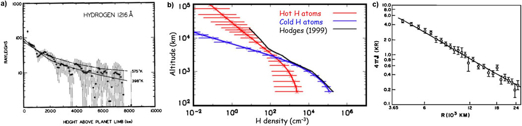
Figure 1. Exosphere profiles derived from Lyman-
During the mid-1980s, Potter and Morgan (1985) detected sodium (Na) from emission lines corresponding to the Fraunhofer sodium D lines in Mercury’s exosphere, and 1 year later, potassium (K) was detected in its resonance line at 769.9 nm (Potter and Morgan, 1986) using a ground-based telescope and spectrometers. The variability in Mercury’s Na exosphere was observed using the Time History of Events and Macroscale Interactions during Substorms (THEMIS) solar telescope (Leblanc et al., 2009). In July 1998, Bida et al. (2000) observed Ca in the planet’s exosphere using the high-resolution Echelle spectrograph at the W. M. Keck I Telescope, focusing on the Ca line (422.674 nm).
In more recent times, the MErcury Surface, Space ENvironment, GEochemistry, and Ranging (MESSENGER) spacecraft observed Na (589.0 and 589.5 nm), Ca (422.7 nm), and H (121.6 nm) emissions (McClintock et al., 2008), and during its second and third flybys, the UVVS instrument also observed the Mg (285.2 nm) line (McClintock et al., 2009; Vervack et al., 2010). On 1st October 2021, the Probing of Hermean Exosphere by UV Spectroscopy (PHEBUS) instrument aboard BepiColombo (Benkhoff et al., 2021) observed He atoms during its first Mercury flyby (Quémerais et al., 2023), marking the first detection of He since the UVS measurements by Mariner 10 in 1974 (Broadfoot et al., 1974).
As shown in Figures 1B, C, extended atomic hydrogen exospheres were observed through Lyman-
One of the main goals for observing particles in exospheres whose densities can then be reproduced by upper atmosphere models is the determination of accurate atmospheric escape rates. Due to Venus being
The ionized fraction of planetary exospheres is mainly detected and characterized through measurements obtained from flight mass spectrometers and particle detectors. The first flight mass spectrometer measurements in Mars’ exosphere were carried out using the Automatic Space Plasma Experiment with a Rotating Analyzer (ASPERA) at the planet’s magnetic boundary (Lundin et al., 1989; Rosenbauer et al., 1989) onboard the Phobos 2 spacecraft. The ASPERA instrument package was designed to study the solar wind interaction with the Martian upper atmosphere so that the plasma and neutral particle environment could be characterized, locally charged particles could be measured, and energetic neutral atoms (ENAs) could be imaged. Measurements were carried out using ENA sensors and ion and electron spectrometers (Barabash et al., 2004), where the neutral particle imager (NPI) measures ENA fluxes within an energy resolution range of
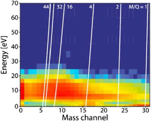
Figure 2. ASPERA-4/IMA mass spectrogram data during a pericenter pass of Venus Express at Venus on 2 July 2014. The white lines indicate the mass per charge of ions obtained from ground calibrations. IMA was not sensitive enough to separate exospheric
Figure 2 shows an IMA energy–mass spectrogram of ions at Venus, where the masses per charge are smeared over the mass channels so that one cannot separate small mass differences (Persson et al., 2019). It should be noted that both instruments also have an integrated ‘neutral particle detector’ (NPD) that measures ENAs that originate via charge exchange with solar wind protons and exospheric H atoms (Lichtenegger et al., 2006; Galli et al., 2008; Lammer et al., 2006). After analyzing MEX ASPERA-3 and MAVEN data, the escape of exospheric
A further example of exospheric particle detectors is the so-called Search for Exospheric Refilling and Emitted Natural Abundances (SERENA) instrument, which is onboard BepiColombo’s MPO spacecraft (Benkhoff et al., 2021). The SERENA instrument package consists of two complementary neutral and two ion particle detectors (Orsini et al., 2021), where the STart from a ROtating Field mass spectrOmeter (STROFIO) measures in situ the low-energy neutral particle composition and density in the energy range
A third technique to derive the density and characterize the exosphere environment of a planetary body is illustrated in Figure 3. In this approach, the exosphere density and outflow rates of the studied target are inferred through a detailed analysis of charge-transfer processes, known as SWCX interaction analysis, between energetic solar wind or exospheric ions and exospheric neutrals. An advantage of this technique is that it does not necessarily need a mass spectrometer onboard the spacecraft. Simon Wedlund et al. (2016); Simon Wedlund et al. (2019a); and Simon Wedlund et al. (2019b) applied this method for the first time to characterize the composition of the dayside neutral coma of the comet 67P/Churyumov–Gerasimenko. The Rosetta Plasma Consortium Ion Composition Analyzer (RPC-ICA) measured the
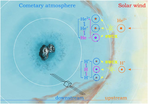
Figure 3. Illustration of solar wind charge exchange interaction processes near the environment of comet 67P/Churyumov–Gerasimenko at approximately 2 AU. The upstream solar wind
A fourth method, which has not been used so often to characterize planetary exospheres—especially their extended regions—is related to plasma physics and in situ magnetic field observations. Various spacecraft such as Galileo (Jupiter system), MEX (Mars; but no magnetometer data), VEX (Venus), MESSENGER (Mercury), and BepiColombo (Mercury) had/have plasma and magnetometers embarked that can detect so-called electromagnetic ICWs. ICWs are generated by temperature anisotropy in plasma that is embedded in a background magnetic field, where the perpendicular temperature is larger than the parallel temperature (Gary, 1991). In a planetary environment, such anisotropy can be obtained by picking up freshly ionized exospheric neutral particles by the background magnetic field. As exospheric neutral atoms become photo-ionized, they start gyrating around the background interplanetary magnetic field (IMF) and get picked up by the solar wind plasma flow. Because the velocity of the newly generated planetary ions is of the order of a couple of km/s, which is very different from the solar wind velocity that reaches hundreds of km/s, the solar wind plasma becomes unstable to different plasma waves via resonant and non-resonant instabilities (Gary, 1991). This instability mechanism has already been shown to take place in any planetary environment with a spatially extended exosphere, such as the Jovian satellites Europa (Volwerk et al., 2001) and Io (Russell et al., 2003; Russell and Blancocano, 2007), Mercury (Schmid et al., 2022; Schmid et al., 2025; Weichbold, 2023; Weichbold et al. 2025), Venus (Russell and Blancocano, 2007; Delva et al., 2008a; Delva et al., 2008b; Delva et al., 2011; Wei et al., 2011), Mars (Russell et al., 1990; Mazelle et al., 2004; Russell and Blancocano, 2007; Delva et al., 2011), and comets (Huddleston et al., 1992a; Huddleston et al., 1992b; Volwerk et al., 2013a; Volwerk et al., 2013b). From the observed wave power of detected ICWs, the photoionization rate, and the ion production rate, one can derive the local density of the corresponding neutral particles, and thus, the related density profiles of the extended exosphere can be reconstructed. Depending on the magnetic field strengths, the gyro radius of the ionized exospheric particles, elements from masses between 1–7 amu, have been detected and analyzed in the space environment around Mercury, Venus, Earth, and Mars; moreover, ICWs have been detected from water-group ions over the E-ring of Saturn and near comets 27P/Grigg–Skjellerup and 1P/Halley. Compared to the previously mentioned exosphere characterization methods, we point out that the ICW technique is advantageous mainly for the following points:
• It is sensitive to very low exospheric number densities and, therefore, is ideally suited for determining exosphere densities in the outer layers of the exosphere.
• It can be used to analyze and separate thermal exospheric particle populations from non-thermal particles (i.e., micrometeorite impact evaporation, sputtering on airless bodies such as Mercury and the Moon, or suprathermal particles in the extended exospheres of Venus, Mars, Earth, etc.).
• It is a technique that is sensitive enough to separate atomic hydrogen from molecular hydrogen, or in the case of Venus, it should be possible to separate suprathermal H atoms from D isotopes.
Although ICWs and related magnetic field data have been studied on various planetary bodies, ICW-related data have only been roughly applied for the characterization of the composition and density of planetary exospheres. This review addresses strengths and future applications of this method. In the following sections, we will focus on the observations and the method where ICWs can be used to reproduce densities of various species in extended exosphere layers, with a focus on Mercury and Venus. We also review and discuss observations of ICWs on Earth, Mars, icy satellites, and comets. In Section 2, we describe the necessary data and parameters that are needed for the analysis of ICWs generated by exospheric pick-up ions. We also emphasize how one can use plasma and magnetic field measurements for the detection of exospheric species that cannot be detected by spectroscopic techniques or particle detectors and how ICW analysis serves as a helpful complementary method to the other techniques mentioned above. Moreover, we describe in detail the technique to retrieve the exospheric neutral density profiles from ICW data. In Section 3, we present and discuss exospheric neutral density profiles of various species derived from the analysis of ICWs at Mercury and Venus. Moreover, we also provide a brief review of available ICW observations in the exosphere environments of Earth, Mars, icy satellites, and comets and how these data can be used to characterize their exospheres in the near future. Section 3 will be completed with an outlook on how future ICW observations at the Jovian satellites by the JUICE mission (Grasset et al., 2013) and on a cometary target studied by the Comet Interceptor (Jones et al., 2024) mission can be complementarily used with mass spectrometers for the characterization of their neutral and ionized exosphere environments. Section 4 provides the conclusion of this work.
2 ICW analysis and retrieval of particle densities in extended exospheres
In space plasma physics, ICWs are longitudinal oscillations of ions and electrons in a magnetized plasma that propagate nearly perpendicular to the magnetic field. The newborn ions are picked up by the IMF, which usually has an angle
In planetary environments, besides the interplanetary magnetic field (IMF), magnetic fields can be intrinsically generated by a magnetic dynamo or induced due to the interaction between a planetary body and the solar wind. In the latter case, the solar wind interaction leads to a bow shock and an induced magnetospheric obstacle close to the planet. In the case of Mercury, Venus, Mars, icy satellites, comets, etc., a substantial part of the upper neutral exosphere is outside the magnetic obstacle and upstream of the bow shock and is, therefore, directly accessible to the solar wind plasma flow (Luhmann and Bauer, 1992). A fraction of the exospheric neutral particles will then be ionized by mainly photoionization, electron impact ionization, and charge exchange. These newborn exospheric ions produce a planetary ion population in the solar wind, where its interaction with the plasma background enables the generation of electromagnetic waves at the ion cyclotron frequency. The produced ICWs can be expected at any location where the pick-up of ionized exospheric neutrals is possible, especially in the extended exosphere regions and upstream of the bow shock (Delva et al., 2008a; Delva et al., 2008b). Unlike plasma waves caused by backward-flowing solar wind ions located in the foreshock region defined by magnetic field lines tangential to the bow shock, ICWs occur anywhere upstream of the environment (Mazelle et al., 2004). In addition, their frequencies are very different, and those backstreaming ions have much lower frequencies than the local IC frequency. Because of this, the observation of ICWs in the upstream region of a planetary body confirms that certain exospheric ions are present and are being carried away by the solar wind into interplanetary space.
Figure 4 shows a schematic illustration of the generation of ICWs around a planetary environment. Neutral exosphere particles (gray dots: 1) are ionized due to photons, electron impact, and charge exchange (purple lines: 2); then, the newborn solar wind picks up exospheric ions and starts to gyrate around the IMF (green lines: 3). By using the solar wind frame as a reference, the exospheric pick-up ions form a secondary distribution in the velocity space that is highly unstable to the cyclotron wave instability, and ICWs (orange lines: 4) are excited. As illustrated in Figure 3, ICWs are mainly generated by pick-up ions upstream of the bow shock with a specific frequency and polarization in the spacecraft frame. The angle between the bulk velocity of the solar wind and the magnetic field vector determines the mechanism for the generation of the ICWs via the growth rate of unstable modes. For perpendicular conditions between the solar wind bulk velocity and the magnetic field, the newly born exospheric ions form a ring-like distribution in velocity space, with the free energy acting as a source for ICWs (Coates et al., 1990; Volwerk et al., 2001; Bertucci et al., 2005; Delva et al., 2008a; Delva et al., 2008b; Delva et al., 2011; Delva et al., 2015).
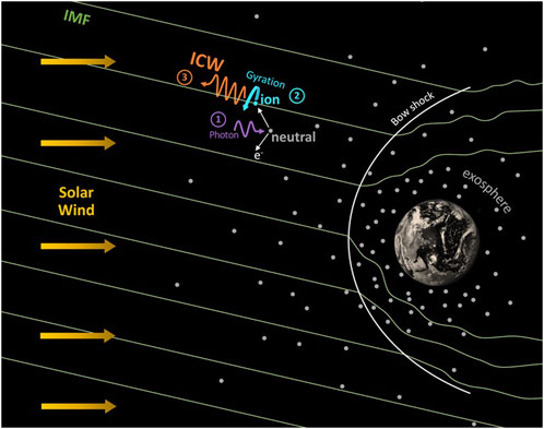
Figure 4. Illustration of the ion cyclotron waves generation mechanism near planetary environments. Exospheric neutral atoms get ionized (gray dots) by solar photons (1: purple line). Newborn ions (2: blue) begin to gyrate around the IMF lines and get picked up by the solar wind plasma flow. In the solar wind frame of reference, these picked up ions from a secondary distribution in the velocity space that is highly unstable to the cyclotron wave instability and ICWs (3: orange line) are excited (Schmid et al., 2022).
For quasi-parallel or antiparallel conditions between the solar wind bulk velocity and the magnetic field, newly born ions form a field-aligned beam of exospheric ions, where the free energy given in Equation 1, determined by Huddleston and Johnstone (1992) is as follows:
which is carried in the parallel drift velocity of the ions relative to the background plasma (Gary, 1991; Gary and Winske, 1993). Here,
To determine the ion pick-up-related ICWs in the magnetic field, the data are split into intervals that can be described as sliding windows; within every interval, the data will be transformed into the mean field-aligned coordinate system (Schmid et al., 2021; Schmid et al., 2022; Weichbold, 2023; Weichbold et al., 2025). These intervals are separated into subintervals, and a fast Fourier transformation and a ‘power spectral density’ (PSD) analysis are then performed (Means, 1972; Samson and Olson, 1980), where further properties of the waves, such as ellipticity and the wave vector, are determined by the off-diagonal elements of the PSD matrix. The calculated values of the subintervals are averaged, and specific selection criteria based on the picked up ions’ characteristics for ICWs can be applied. By fulfilling this selection criterion, the fluctuations within this interval are then identified as pick-up ion-based ICWs. Since the gyrofrequency of the picked up ions is given by the charge of the ion multiplied by the inverse of the particle mass and the total magnetic field strength, it is possible to distinguish between different exospheric pick-up ion species. The specific frequency of ICWs in the spacecraft frame enables a clear distinction between plasma waves that are generated by exospheric ions and those that belong to solar wind protons. Waves that are produced by solar wind protons that are reflected by the bow shock are observed with a much lower frequency than ICWs that originate from exospheric ions and are limited to the foreshock region (Shan et al., 2014).
One can analyze the ICWs that are generated by picked up ions using solar wind and plasma data such as solar wind velocity and density (Fränz et al., 2017; Rojas Mata et al., 2022). The pick-up ion number density
where
with the electric charge
The waves will be observed at the local ion gyrofrequency in the spacecraft frame and with specific left-hand polarization due to the anomalous Doppler effect (Mazelle and Neubauer, 1993). This fact immediately excludes confusion with ULF waves generated by solar wind protons back-streaming from the bow shock, which will be observed at the spacecraft at frequencies much lower than the cyclotron frequency (Gary, 1991) and occur only within the foreshock.
Moreover, it is important to note that one can distinguish ICWs from exospheric particles with masses that lie close together, such as atomic and molecular hydrogen or H atoms and D isotopes. In this context, as shown in Figure 2, it was not possible to separate
For the analysis of ICWs, the following identification criteria can be defined (Schmid et al., 2022) after one has identified ICW events in the space environment around a planetary body. To identify the pick-up produced ICWs, one can use magnetic field observations of approximately 20 Hz applied to the following steps within a sliding interval that lasts
• Magnetic field data are transformed into a mean-field-aligned (MFA) coordinate system.
• Fourier-transformed
• The diagonal elements of the power spectral density matrix represent the parallel and perpendicular in-phase power densities relative to the mean magnetic field. The ellipticity and the handedness of the observed electromagnetic wave are inferred from the complex off-diagonal elements to the power spectral density matrix, where negative/positive signs refer to the left/right-handed polarization of the wave in the spacecraft frame (Arthur et al., 1976; Samson and Olson, 1980; Schmid et al., 2022).
• The polarization degree of each subinterval is determined.
Considering the aforementioned steps, the arithmetic means of the ellipticities and power densities of the subintervals are calculated. Another condition for ICWs that are produced by exospheric pick-up ions is that the observed frequency in the spacecraft frame is close to the local ion gyrofrequency
where
• To account for a power maxima below the
• Within the frequency range
• The polarization degree of all subintervals is required to be larger than 0.7 within
• To ensure that the ion cyclotron mode dominates the observed wave, the maximum of the fluctuating perpendicular power density of the mean magnetic field should remain within the limits of
Figure 5 shows examples of ICWs identified from the analysis of magnetic field data of MESSENGER, which are generated by exospheric
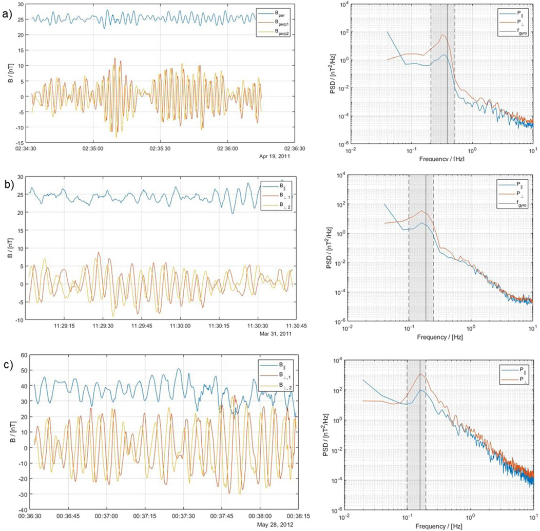
Figure 5. Examples of identified ICWs from MESSENGER magnetic field data and power spectra for
The propagation speeds of ICWs are less than the local Alfvén velocity
3 Exosphere characterization by ICW-data analysis throughout the solar system
3.1 Mercury
Mercury is considered an airless body like Earth’s Moon, where the exobase level is at the planet’s surface, and thus, it is directly exposed to mainly solar ions, electrons, and photons from the infrared to X-rays (Lammer et al., 2022; Wurz et al., 2022) and additionally to meteoroid fluxes (Wurz et al., 2022). The exposure of Mercury’s surface to these exogenic sources modifies the surface by altering the chemical makeup and optical properties. Moreover, due to the interaction with these sources, a neutral silicate exosphere with an ionized component is produced.
3.1.1 H atoms in Mercury’s extended exosphere
Until now, only two spacecraft have investigated the environment near Mercury: Mariner 10, which conducted three flybys during 1974–1975, and MESSENGER, four decades later. As briefly discussed in Section 1, early spectroscopic observations by Mariner 10 that were confirmed by MESSENGER showed that Mercury has an extended exosphere that is populated by neutral atomic hydrogen. Schmid et al. (2022) derived for the first time an altitude–density profile of the planet’s extended H exosphere from in situ magnetic field measurements by MESSENGER. The observed H+ ions produce the previously mentioned ICWs, which can then be identified in the magnetic field data. Schmid et al. (2022) analyzed these data and derived the local H number density that is necessary to excite the related ICWs. The results reveal an extended atomic H exosphere between
The blue dots in Figure 6A show the altitude dependence of the ICW-based and derived H atom number density from MESSENGER magnetic field data that were analyzed and adopted from Weichbold (2023). The radial distance in Mercury’s radii (
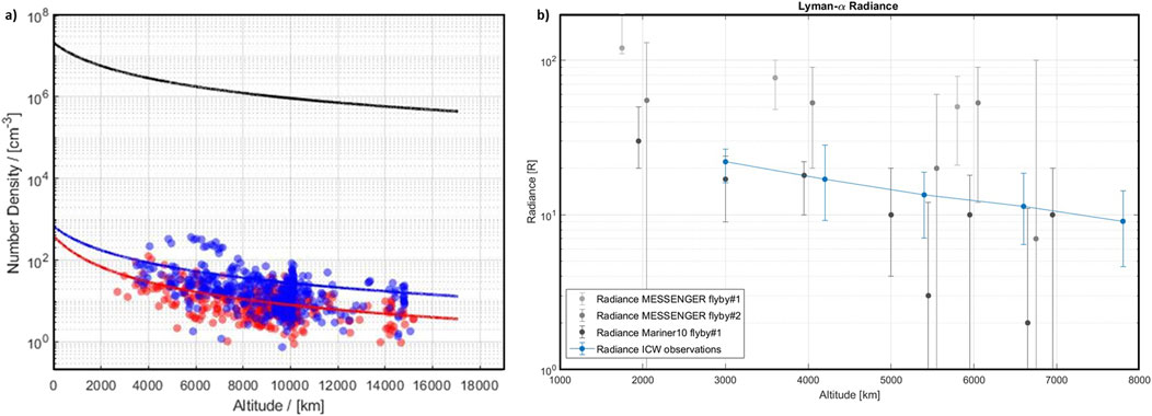
Figure 6. Panel (A): Altitude density profiles of exospheric H atoms (blue dots) and
3.1.2 Exospheric H2 molecules
Recently, Weichbold (2023) obtained the first number density profile of
One explanation for this result might be that the dissociation and ionization rates of
As pointed out below, ICWs generated by energetic neutral H atoms are also observed in Earth’s magnetosphere environment over the polar cusp (Wei et al., 2011). Since the pick-up process inside a magnetosphere is more complex compared to a planet without an intrinsic magnetic field like Venus or Mars—due to the magnetic field variations with altitude and latitude—the observed ICWs exhibit more variable properties. Since Mercury also has an intrinsic magnetic field like Earth, one can expect that similar processes will occur in the planet’s exosphere. In analogy to Earth, one can expect that a population of energetic neutral H atoms can be produced via interlinked charge exchange and ion pick-up processes over Mercury’s cusp, from where they may spread into the exosphere from their source region. Exospheric H atoms will be ionized and accelerated as a picked up
The red dots in Figure 6A show the density profile of neutral
3.1.3 Mercury’s extended He exosphere
He in Mercury’s exosphere was first detected through remote spectroscopic observations of the Ultraviolet 14 Visible Spectrometer (UVVS) instruments in Mercury’s exosphere during the Mariner 10 flybys between 1974 and 1975. Broadfoot et al. (1974), Hartle et al. (1975), Weichbold (2023), and Weichbold et al. (2025) analyzed the available MESSENGER magnetic field and plasma data from 2011–2015 and inferred in situ the He content in the extended exosphere between
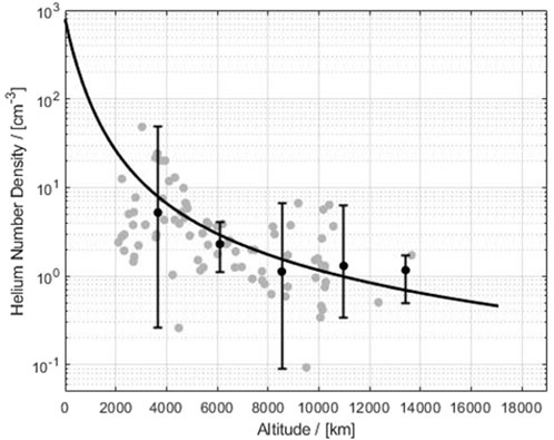
Figure 7. Altitude density profile of exospheric He atoms (gray dots) around Mercury. The gray dots depict the derived He number density related to analyzed ICW events that correspond to
3.1.4 Search and detection of meteoritic Li in the Mercury’s exosphere
According to Killen et al. (2007), one can also expect that unknown components such as Li populate Mercury’s exosphere. The abundance of Li in the solar system is
Nearly three decades later, Schmid et al. (2025) reported for the first time the in situ discovery of Li in Mercury’s exosphere, which is released from the surface by sporadic impact events of m-size meteoroids. The exospheric Li was discovered through the detection of Li-based ICWs, derived similarly to the aforementioned H,
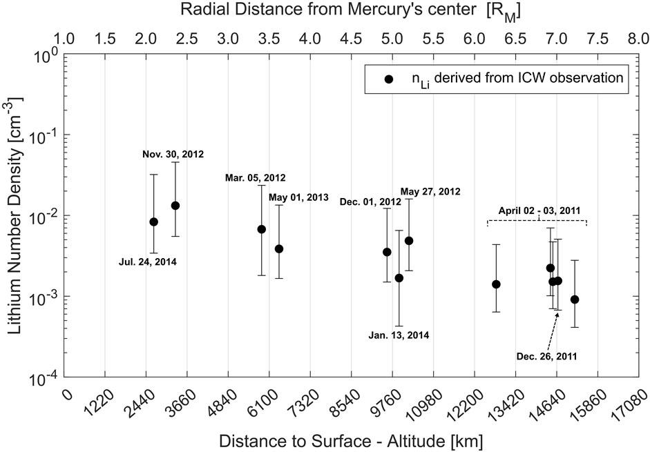
Figure 8. Average Li densities as a function of height (black dots, including error bars) related to the detected meteoritic impact events in Mercury’s exosphere between April 2011 and July 2014. Adopted from Schmid et al. (2025).
3.2 Venus
In addition to available Lyman-
However, we note that by revisiting the
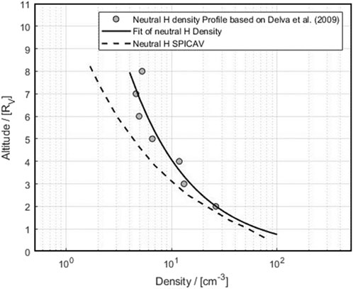
Figure 9. Venus’ exospheric H profile (black line) inferred from
The previously mentioned unit error and the simplified density estimations in their analysis also explain why the authors mistakenly believed that their inferred neutral gas density was much higher than expected. After the discovery and clarification of this inconsistency, we plan to soon reanalyze the plasma and magnetic field data and related ICWs in detail. This reanalysis will also include the more accurate approach and methods as described in previous sections and by Schmid et al. (2025) and Weichbold (2025). Moreover, it will also contain the search for ICWs that are generated by exospheric
The deuterium to hydrogen (D/H) ratio on Venus shows an approximately 100-fold enrichment compared to that on Earth (Donahue et al., 1982), which is a fundamental constraint on models for its evolution of the water inventory and atmosphere (Lammer et al., 2020; Gillmann et al., 2022). From VEX, it is known that Venus has thick clouds and aerosol particles of
For the explanation of the extended H exosphere at Venus shown in Figures 1B, 9, photochemical and charge exchange processes are responsible for the production of suprathermal H atoms (Rodriguez et al., 1984; Hodges, 1999; Lammer et al., 2006; Shematovich et al., 2014; Chaffin et al., 2024). Because suprathermal D isotopes will also undergo the same reactions and processes, one can expect that D isotopes should also populate Venus’ exosphere. Contrary to Mars’ exosphere, Venus exosphere does not contain
By reproducing accurate extended exospheric H and D distributions, it will, for the first time, be possible to obtain accurate loss rates of suprathermal H atoms and D atoms over the entire solar activity cycle. Together with the known ion loss rates, the total escape rates of H and D particles as a function of solar activity can finally be determined. This will also provide the ratio of H loss versus D loss, a crucial factor for evaluating the evolution of the D/H ratio and its connection to Venusian water inventory. The activity variation between the solar minimum and maximum can then be used as a proxy for covering the period of the Sun’s average EUV flux evolution from present the day to the time Venus experienced a resurfacing event
From this brief overview of the extended hydrogen exosphere at Venus, it is apparent that important work remains to be done to better understand and quantify the efficiency of the various processes related to the production of suprathermal hydrogen and D isotopes. This understanding is essential for reliably reconstructing and constraining the extended hydrogen and deuterium population in Venus’ exosphere.
3.3 ICWs at Earth’s polar cusps
Contrary to Venus, Earth possesses an intrinsic magnetic field like Mercury that builds a magnetospheric obstacle or standoff distance from the planet’s surface at the subsolar point of
On Earth, ICWs are observed over the cusp regions in the frequency ranges of
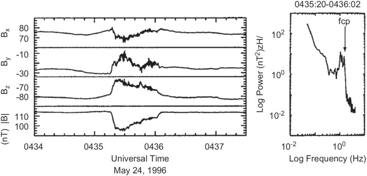
Figure 10. Example of a time series and power spectra of a typical
3.4 Mars’ extended H exosphere
On Mars, ICWs were first discovered during the Phobos mission at approximately 2–3 Mars radii with frequencies that correspond to ionized exospheric picked up hydrogen atoms (Russell et al., 1990). These findings are supported by the observations of the pick-up of
Figure 11 shows an example of ICWs observed by MGS (Wei and Russell, 2006). The x-axis points from Mars to the Sun, the z-axis points upward and perpendicular to the orbital plane, and the y-axis completes a right-handed system. Similar to Mercury and Venus, the ICWs on Mars indicate that the planet has an extended hydrogen exosphere. The production of this extended hydrogen exosphere around Mars is illustrated according to Wei and Russell (2006) in Figure 11. Similar to Venus, close to Mars, exospheric H atoms are ionized and picked up due to the solar wind plasma interaction with the exosphere. This creates the detected ICWs near the planet. It is also expected that charge exchange with solar wind protons produces an energetic H atom population that is transported to greater distances where they are again re-ionized so that ICWs can be generated downstream of Mars and far to one side of the planet. Moreover, the analysis of the magnetic field and plasma data revealed an asymmetry in the direction of the interplanetary electric field, which is also found in numerical modeling (Brecht, 1990; Modolo et al., 2005). The reason for this asymmetry is related to the effects of the finite gyro radius, which is approximately 0.3 Mars radii for pick-up
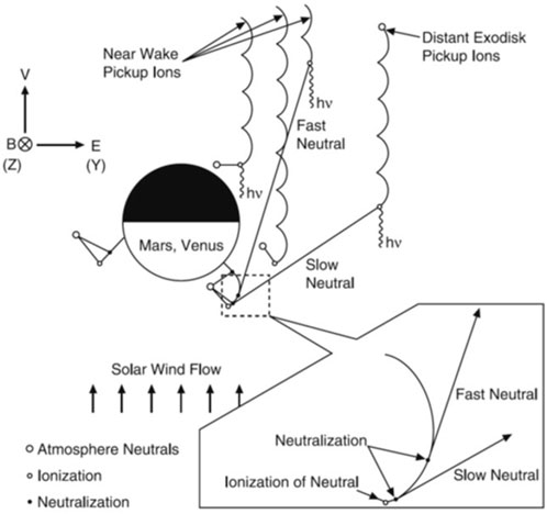
Figure 11. Mechanism for producing an extended H exosphere around Mars. Detailed describtions are provided in the main text [adopted from Wei and Russell (2006)].
Since D has also been discovered in the Martian atmosphere (Owen et al., 1988) and the D/H ratio shows that D is enriched relative to atomic H by a factor of
In the future, the ‘Mars-Magnetosphere, ATmosphere, Ionosphere, and Space-weather SciencE’ (M-Matisse) mission, which will study Mars using two spacecraft equipped with identical set of instruments to observe the planet simultaneously from two different locations in space, will be well-equipped to study ICWs. This mission can be used for the analysis of solar wind influences on the planet’s exosphere, outer regions, the magnetic environment, and the ionosphere.
3.5 Jovian system
The giant planets in our solar system have large moons that interact with the magnetospheric plasma. These interactions can lead to the sputtering of surface particles (Watson, 1982) or volcanic activity—either magmatic, as observed in the case of Io (Smith et al., 1979; Consolmagno, 1979), or cryogenic, as observed in the cases of Europa and Enceladus (Fagents, 2003; Hansen et al., 2006). The ionization of these particles through UV radiation or electron impacts leads to pick-up by the magnetospheric magnetic field. The giant planets rotate much faster than the Keplerian velocity of the moons, and thereby, the newly generated ions are energized and create a ring (beam) distribution in velocity space, which is unstable for ICWs and mirror modes.
The pick-up ICWs at the moon of a giant planet were first detected during Galileo’s Jupiter orbit insertion flyby of Io (Huddleston et al., 1997; Warnecke et al., 1997) using a magnetometer (Kivelson et al., 1992). Strong, left-handed polarized waves at the cyclotron frequency of
The Galileo magnetometer data were also investigated for other Galilean satellites. Because of the stronger magnetic field strengths in the Jovian magnetosphere, it is possible to measure the waves generated by heavier ions. At Europa, it was found that many different ions sputtered from the surface, such as Na, Cl, K, and
A study of the three icy Galilean moons found that the pick-up and consequent generation of ICWs varies with the moon’s location and the spacecraft flyby (Volwerk et al., 2010). On the upstream side of Europa, pick-up of
where
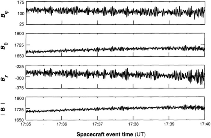
Figure 12. Observed ICWs in the vicinity of Io. Expanded data from 17:35 to 17:40 UT (Kivelson et al., 1996c).
At Ganymede, the pick-up ICW signatures are significantly less because of the internal magnetic field of this moon (Kivelson et al., 1996a;; Kivelson et al., 1996b), which creates a mini-magnetosphere with various wave modes (Volwerk et al., 1999). However, during one flyby, before Galileo entered the region of closed field lines, a broad signature around the
Callisto poses a problem for the analysis of sputter ion pick-up because of the low magnetic field strength of
In the future, the Jupiter Icy Moons Explorer (JUICE) spacecraft, expected to arrive in the Jupiter system in 2031, is anticipated to investigate ICWs and exospheric species of the icy satellites through correlated efforts involving the Jovian-magnetometer (J-MAG), the Radio and Plasma Wave Investigation (RPWI), and the Particle Environment Package (PEP) instruments, along with their teams.
3.6 Kronian system
Saturn’s system consists of a multitude of moons and rings, including well-known objects like Titan, Enceladus, the E-ring, and, more recently, Mimas, which is expected to have a recently formed ocean underneath its icy crust (Lainey et al., 2024).
The first evidence for ICWs in the Kronian system came from Pioneer 11 observations in the E-ring in the neighborhood of Dione’s L-shell (Smith and Tsurutani, 1983), and although the generation mechanism is assumed to be the ion cyclotron resonance, these are not from local pick-up of freshly ionized particles but likely generated by a temperature anisotropy in the
Cassini, with its magnetometer (Dougherty et al., 2004), flew over the E-ring and measured clear ICWs around frequencies of water-group ions (
Enceladus was found to have water plumes in its southern hemisphere (Porco et al., 2006), which also had a clear signature in the magnetometer measurements (Dougherty et al., 2006). During two Enceladus flybys, there were clear cyclotron wave signatures in the magnetometer data, mainly downstream of the moon. The period of the waves is consistent with the pick-up of
However, the detection of ICWs remained elusive in the almost 100 flybys of Titan by Cassini. Only two events have been found during the T63 and T98 flybys (Russell et al., 2016): in the former,
3.7 Comets
Comets start their outgassing when their orbits cross Jupiter’s orbit when the solar irradiance is strong enough to start the sublimation of volatiles in the nucleus. This neutral gas cloud that is created reacts with the solar UV radiation and gets ionized, and it will also interact with the solar wind, creating a bow shock and a coma, various boundaries, and the diamagnetic cavity (Goetz et al., 2022; Goetz et al., 2023).
The freshly ionized particles in the coma will be picked up by the solar wind and can generate ICWs. There have been a few missions to comets: Giotto encountered comet 27P/Grigg–Skjellerup, and ICWs were measured near the
During the Rosetta mission around comet 67P/Churyumov–Gerasimenko, no evidence of ICWs was obtained from the magnetometer data, which could be caused by the relatively weak outgassing rates at approach and the too-short transport time of the picked up ions for the waves to grow to a detectable level. Because the target body for the Comet Interceptor mission at the end of this decade is not yet known (Jones et al., 2024), it is not clear if ICWs and related research can be carried out for the characterization of the Comet Interceptor’s target. However, one can speculate that the novelty of three-point magnetic measurements when the Comet Interceptor mission is fully deployed in and around the target comet, albeit a nominal mission duration of at most a few hours, will allow us to derive a spatial and temporal distribution of cometary exospheric species from hydrogen to heavier neutral molecular species.
4 Conclusion
We have shown that a detailed analysis of observed ion cyclotron waves generated by exospheric pick-up ions can be used to derive the neutral densities of exospheric particles in extended exosphere layers. The method is mainly applicable to light elements (H,
Author contributions
HL: conceptualization, investigation, writing–original draft, and writing–review and editing. DS: data curation, investigation, methodology, software, visualization, and writing–review and editing. MV: investigation, methodology, and writing–review and editing. FW: methodology, visualization, and writing–review and editing. CW: investigation and writing–review and editing. AV: investigation and writing–review and editing. MD: methodology and writing–review and editing.
Funding
The author(s) declare that financial support was received for the research, authorship, and/or publication of this article. HL and FW thank the Austrian Science Fund (FWF) for the support of the VeReDo research project, grant I6857N. CW was funded by the Austrian Science Fund (FWF) project 10.55776/P35954.
Conflict of interest
The authors declare that the research was conducted in the absence of any commercial or financial relationships that could be construed as a potential conflict of interest.
The author(s) declared that they were an editorial board member of Frontiers, at the time of submission. This had no impact on the peer review process and the final decision.
Correction note
A correction has been made to this article. Details can be found at: 10.3389/fspas.2025.1667857.
Publisher’s note
All claims expressed in this article are solely those of the authors and do not necessarily represent those of their affiliated organizations, or those of the publisher, the editors, and the reviewers. Any product that may be evaluated in this article, or claim that may be made by its manufacturer, is not guaranteed or endorsed by the publisher.
Footnotes
1Carruthers Geocorona Observatory: https://science.nasa.gov/mission/carruthers-geocorona-observatory/
References
Anders, E., and Grevesse, N. (1989). Abundances of the elements: meteoritic and solar. Geochim. Cosmochim. Acta 53, 197–214. doi:10.1016/0016-7037(89)90286-X
Anderson, J., and Donald, E. (1976). The mariner 5 ultraviolet photometer experiment: analysis of hydrogen lyman-alpha data. J. Geophys. Res. 81, 1213–1216. doi:10.1029/JA081i007p01213
Anderson, J., Donald, E., and Hord, C. W. (1971). Mariner 6 and 7 ultraviolet spectrometer experiment: analysis of hydrogen lyman-alphaalpha data. J. Geophys. Res. 76, 6666. doi:10.1029/JA076i028p06666
Arthur, C. W., McPherron, R. L., and Means, J. D. (1976). A comparative study of three techniques for using the spectral matrix in wave analysis. Radio Sci. 11, 833–845. doi:10.1029/RS011i010p00833
Barabash, S., Dubinin, E., Pisarenko, N., Lundin, R., and Russell, C. T. (1991). Picked-up protons near Mars: Phobos observations. Geophys. Res. Lett. 18, 1805–1808. doi:10.1029/91GL02082
Barabash, S., Fedorov, A., Lundin, R., and Sauvaud, J.-A. (2007). Martian atmospheric erosion rates. Science 315, 501–503. doi:10.1126/science.1134358
Barabash, S., Lundin, R., Andersson, H., Gimholt, J., Holmström, M., Norberg, O., et al. (2004). “ASPERA-3: analyser of space plasmas and energetic ions for Mars Express,” in Mars express: the scientific payload. Editors A. Wilson, and A. Chicarro (Noordwijk, Netherlands: ESA Special Publication), 1240, 121–139.
Barth, C. A., Fastie, W. G., Hord, C. W., Pearce, J. B., Kelly, K. K., Stewart, A. I., et al. (1969). Mariner 6: ultraviolet spectrum of Mars upper atmosphere. Science 165, 1004–1005. doi:10.1126/science.165.3897.1004
Bauer, S. J., and Lammer, H. (2004). Planetary aeronomy: atmosphere environments in planetary systems. Berlin, Heidelberg, New York: Springer.
Benkhoff, J., Murakami, G., Baumjohann, W., Besse, S., Bunce, E., Casale, M., et al. (2021). BepiColombo - mission overview and science goals. Space Sci. Rev. 217, 90. doi:10.1007/s11214-021-00861-4
Bertaux, J. L., Blamont, J., Marcelin, M., Kurt, V. G., Romanova, N. N., and Smirnov, A. S. (1978). Lyman-alpha observations of venera-9 and 10 I. The non-thermal hydrogen population in the exosphere of venus. Planet. Space Sci. 26, 817–831. doi:10.1016/0032-0633(78)90105-8
Bertaux, J. L., Lepine, V. M., Kurt, V. G., and Smirnov, A. S. (1982). Altitude profile of H in the atmosphere of Venus from Lyman α observations of Venera 11 and Venera 12 and origin of the hot exospheric component. Icarus 52, 221–244. doi:10.1016/0019-1035(82)90110-5
Bertaux, J.-L., Vandaele, A.-C., Korablev, O., Villard, E., Fedorova, A., Fussen, D., et al. (2007). A warm layer in Venus’ cryosphere and high-altitude measurements of HF, HCl, H2O and HDO. Nature 450, 646–649. doi:10.1038/nature05974
Bertucci, C., Mazelle, C., and Acuña, M. H. (2005). Interaction of the solar wind with Mars from Mars global surveyor MAG/ER observations. J. Atmos. Solar-Terrest. Phys. 67, 1797–1808. doi:10.1016/j.jastp.2005.04.007
Bida, T. A., Killen, R. M., and Morgan, T. H. (2000). Discovery of calcium in Mercury’s atmosphere. Nature 404, 159–161. doi:10.1038/35004521
Brecht, S. H. (1990). Magnetic asymmetries of unmagnetized planets. Geophys. Res. Lett. 17, 1243–1246. doi:10.1029/GL017i009p01243
Broadfoot, A. L., Kumar, S., Belton, M. J. S., and McElroy, M. B. (1974). Mercury’s atmosphere from mariner 10: preliminary results. Science 185, 166–169. doi:10.1126/science.185.4146.166
Broadfoot, A. L., Shemansky, D. E., and Kumar, S. (1976). Mariner 10: Mercury atmosphere. Geophys. Res. Lett. 3, 577–580. doi:10.1029/GL003i010p00577
Chaffin, M. S., Cangi, E. M., Gregory, B. S., Yelle, R. V., Deighan, J., Elliott, R. D., et al. (2024). Venus water loss is dominated by HCO+ dissociative recombination. Nature 629, 307–310. doi:10.1038/s41586-024-07261-y
Chamberlain, J. W. (1963). Planetary coronae and atmospheric evaporation. Planet. Space Sci. 11, 901–960. doi:10.1016/0032-0633(63)90122-3
Chaufray, J. Y., Bertaux, J. L., Quémerais, E., Villard, E., and Leblanc, F. (2012). Hydrogen density in the dayside venusian exosphere derived from Lyman-α observations by SPICAV on Venus Express. Icarus 217, 767–778. doi:10.1016/j.icarus.2011.09.027
Chaufray, J. Y., Gonzalez-Galindo, F., Leblanc, F., Modolo, R., Vals, M., Montmessin, F., et al. (2024). Simulations of the hydrogen and deuterium thermal and non-thermal escape at Mars at Spring Equinox. Icarus 418, 116152. doi:10.1016/j.icarus.2024.116152
Chirakkil, K., Deighan, J., Chaffin, M. S., Jain, S. K., Lillis, R. J., Raghuram, S., et al. (2024). EMM EMUS observations of hot oxygen corona at Mars: radial distribution and temporal variability. J. Geophys. Res. Space Phys. 129, e2023JA032342. doi:10.1029/2023JA032342
Coates, A. J., Johnstone, A. D., Huddleston, D. E., Wilken, B., Jockers, K., Borg, H., et al. (1993). Pickup water group ions at comet Grigg-Skjellerup. Geophys. Res. Lett. 20, 483–486. doi:10.1029/93gl00174
Coates, A. J., Johnstone, A. D., Kessel, R. L., Huddleston, D. E., and Wilken, B. (1990). Plasma parameters near the Comet Halley bow shock. J. Geophys. Res. 95, 20701–20716. doi:10.1029/JA095iA12p20701
Consolmagno, G. J. (1979). Sulfur volcanoes on Io. Science 205, 397–398. doi:10.1126/science.205.4404.397
Cowee, M. M., and Gary, S. P. (2012). Electromagnetic ion cyclotron wave generation by planetary pickup ions: one-dimensional hybrid simulations at sub-Alfvénic pickup velocities. J. Geophys. Res. Space Phys. 117, A06215. doi:10.1029/2012JA017568
Cowee, M. M., Gary, S. P., and Wei, H. Y. (2012). Pickup ions and ion cyclotron wave amplitudes upstream of Mars: first results from the 1D hybrid simulation. Geophys. Res. Lett. 39, L08104. doi:10.1029/2012GL051313
Cowee, M. M., Gary, S. P., Wei, H. Y., Tokar, R. L., and Russell, C. T. (2010). An explanation for the lack of ion cyclotron wave generation by pickup ions at Titan: 1-D hybrid simulation results. J. Geophys. Res. 115, A10224. doi:10.1029/2010JA015769
Cowee, M. M., Russell, C. T., Strangeway, R. J., and Blanco-Cano, X. (2007). One-dimensional hybrid simulations of obliquely propagating ion cyclotron waves: application to ion pickup at Io. J. Geophys. Res. Space Phys. 112, A06230. doi:10.1029/2006JA012230
Cravens, T. E., Gombosi, T., and Nagy, A. F. (1980). Hot hydrogen in the exosphere of Venus. Nature 283, 178–180. doi:10.1038/283178a0
Deighan, J., Chaffin, M. S., Chaufray, J. Y., Stewart, A. I. F., Schneider, N. M., Jain, S. K., et al. (2015). MAVEN IUVS observation of the hot oxygen corona at Mars. Geophys. Res. Lett. 42, 9009–9014. doi:10.1002/2015GL065487
Delva, M., Bertucci, C., Volwerk, M., Lundin, R., Mazelle, C., and Romanelli, N. (2015). Upstream proton cyclotron waves at Venus near solar maximum. J. Geophys. Res. Space Phys. 120, 344–354. doi:10.1002/2014JA020318
Delva, M., Mazelle, C., and Bertucci, C. (2011). Upstream ion cyclotron waves at venus and Mars. Space Sci. Rev. 162, 5–24. doi:10.1007/s11214-011-9828-2
Delva, M., Volwerk, M., Mazelle, C., Chaufray, J. Y., Bertaux, J. L., Zhang, T. L., et al. (2009). Hydrogen in the extended venus exosphere. Geophys. Res. Lett. 36, L01203. doi:10.1029/2008GL036164
Delva, M., Zhang, T. L., Volwerk, M., Magnes, W., Russell, C. T., and Wei, H. Y. (2008a). First upstream proton cyclotron wave observations at Venus. Geophys. Res. Lett. 35, L03105. doi:10.1029/2007GL032594
Delva, M., Zhang, T. L., Volwerk, M., Vörös, Z., and Pope, S. A. (2008b). Proton cyclotron waves in the solar wind at Venus. J. Geophys. Res. (Planets) 113, E00B06. doi:10.1029/2008JE003148
Donahue, T. M. (1999). New analysis of hydrogen and deuterium escape from venus. Icarus 141, 226–235. doi:10.1006/icar.1999.6186
Donahue, T. M., Hoffman, J. H., Hodges, R. R., and Watson, A. J. (1982). Venus was wet: a measurement of the ratio of deuterium to hydrogen. Science 216, 630–633. doi:10.1126/science.216.4546.630
Dougherty, M. K., Kellock, S., Southwood, D. J., Balogh, A., Tsurutani, E. J. S. B. T., Gerlach, B., et al. (2004). The Cassini magnetic field investigation. Space Sci. Rev. 114, 331–383. doi:10.1007/978-1-4020-2774-1_4
Dougherty, M. K., Khurana, K. K., Neubauer, F. M., Russell, C. T., Saur, J., Leisner, J. S., et al. (2006). Identification of a dynamic atmosphere at Enceladus with the Cassini magnetometer. Science 311, 1406–1409. doi:10.1126/science.1120985
Erlandson, R. E., Zanetti, L. J., Potemra, T. A., Andre, M., and Matson, L. (1988). Observation of electromagnetic ion cyclotron waves and hot plasma in the polar cusp. Geophys. Res. Lett. 15, 421–424. doi:10.1029/GL015i005p00421
Fagents, S. A. (2003). Considerations for effusive cryovolcanism on Europa: the post-Galileo perspective. J. Geophys. Res. 108, 5139. doi:10.1029/2003JE002128
Fränz, M., Echer, E., Marques de Souza, A., Dubinin, E., and Zhang, T. L. (2017). Ultra low frequency waves at venus: observations by the venus express spacecraft. Planet. Space Sci. 146, 55–65. doi:10.1016/j.pss.2017.08.011
Galli, A., Wurz, P., Kallio, E., Ekenbäck, A., Holmström, M., Barabash, S., et al. (2008). Tailward flow of energetic neutral atoms observed at Mars. J. Geophys. Res. (Planets) 113, E12012. doi:10.1029/2008JE003139
Gary, S. P. (1991). Electromagnetic ion/ion instabilities and their consequences in space plasmas - a review. Space Sci. Rev. 56, 373–415. doi:10.1007/BF00196632
Gary, S. P., and Winske, D. (1993). Simulations of ion cyclotron anisotropy instabilities in the terrestrial magnetosheath. J. Geophys. Res. 98, 9171–9179. doi:10.1029/93JA00272
Gillmann, C., Way, M. J., Avice, G., Breuer, D., Golabek, G. J., Höning, D., et al. (2022). The long-term evolution of the atmosphere of venus: processes and feedback mechanisms. Space Sci. Rev. 218, 56. doi:10.1007/s11214-022-00924-0
Glassmeier, K. H., Motschmann, U., Mazalle, C., Neubauer, F. M., Sauer, K., Fuselier, S. A., et al. (1993). Mirror modes and fast magnetoaucoustic waves near the magnetic pileup boundary of comet P/Halley. J. Geophys. Res. 98, 20955–20964. doi:10.1029/93JA02582
Glassmeier, K.-H., and Neubauer, F. M. (1993). Low-frequency electromagnetic plasma waves at comet P/Grigg-Skjellerup: overview and spectral characteristics. J. Geophys. Res. 98, 20921–20935. doi:10.1029/93ja02583
Goetz, C., Behar, E., beth, A., Bodewits, D., Bromley, S., Burch, J., et al. (2022). The plasma environment of comet 67P/Churyumov-Gerasimenko. Space Sci. Rev. 218, 65. doi:10.1007/s11214-022-00931-1
Goetz, C., Gunell, H., Volwerk, M., Beth, A., Erkisson, A., Galand, M., et al. (2023). Cometary plasma science - open science questions for future space missions. Exp. Astro. 54, 1129–1167. doi:10.1007/s10686-021-09783-z
Grasset, O., Dougherty, M. K., Coustenis, A., Bunce, E. J., Erd, C., Titov, D., et al. (2013). JUpiter ICy moons Explorer (JUICE): an ESA mission to orbit Ganymede and to characterise the Jupiter system. Planet. Space Sci. 78, 1–21. doi:10.1016/j.pss.2012.12.002
Halekas, J. S. (2017). Seasonal variability of the hydrogen exosphere of Mars. J. Geophys. Res. (Planets) 122, 901–911. doi:10.1002/2017JE005306
Halekas, J. S., and McFadden, J. P. (2021). Using solar wind helium to probe the structure and seasonal variability of the martian hydrogen corona. J. Geophys. Res. (Planets) 126, e07049. doi:10.1029/2021je007049
Halekas, J. S., Taylor, E. R., Dalton, G., Johnson, G., Curtis, D. W., McFadden, J. P., et al. (2015). The solar wind ion analyzer for MAVEN. Space Sci. Rev. 195, 125–151. doi:10.1007/s11214-013-0029-z
Hansen, C. J., Esposito, L., Stewart, A. I. F., Colwell, J., Hendrix, A., Pryor, W., et al. (2006). Enceladus’ water vapor plume. Science 311, 1422–1425. doi:10.1126/science.1121254
Hartle, R. E., Curtis, S. A., and Thomas, G. E. (1975). Mercury’s helium exosphere. J. Geophys. Res. 80, 3689–3692. doi:10.1029/JA080i025p03689
Hodges, R. R. (1999). An exospheric perspective of isotopic fractionation of hydrogen on Venus. J. Geophys. Res. 104, 8463–8471. doi:10.1029/1999JE900006
Holsclaw, G. M., Deighan, J., Almatroushi, H., Chaffin, M., Correira, J., Evans, J. S., et al. (2021). The Emirates Mars ultraviolet spectrometer (EMUS) for the EMM mission. Space Sci. Rev. 217, 79. doi:10.1007/s11214-021-00854-3
Huddleston, D. E., Coates, A. J., and Johnstone, A. D. (1992a). Correction to ‘Predictions of the solar wind interaction with comet Grigg-Skjellerup by eds D. E. Huddleston, and A. J. Coates, A. D. Johnst. Geophys. Res. Lett. 19, 1319. doi:10.1029/92GL01330
Huddleston, D. E., Coates, A. J., and Johnstone, A. D. (1992b). Predictions of the solar wind interaction with Comet Grigg-Skjellerup. Geophys. Res. Lett. 19, 837–840. doi:10.1029/92GL00639
Huddleston, D. E., and Johnstone, A. D. (1992). Relationship between wave energy and free energy from pickup ions in the Comet Halley Environment. J. Geophys. Res. 97, 12217–12230. doi:10.1029/92JA00726
Huddleston, D. E., Strangeway, R. J., Warnecke, J., Russell, C. T., and Kivelson, M. G. (1998). Ion cyclotron waves in the Io torus: wave dispersion, free energy analysis, and SO2+ source rate estimates. J. Geophys. Res. 103, 19887–19899. doi:10.1029/97JE03557
Huddleston, D. E., Strangeway, R. J., Warnecke, J., Russell, C. T., Kivelson, M. G., and Bagenal, F. (1997). Ion cyclotron waves in the Io torus during the Galileo encounter: warm plasma dispersion analysis. Geophys. Res. Lett. 24, 2143–2146. doi:10.1029/97GL01203
Huddleston, D. E., Strangway, R. J., Blanco-Cano, X., Russell, C. T., Kivelson, M. G., and Khurana, K. K. (1999). Mirror-mode structures at the Galileo-Io flyby: instability criterion and dispersion analysis. J. Geophys. Res. 104, 17479–17489. doi:10.1029/1999JA900195
Huebner, W. F., and Mukherjee, J. (2015). Photoionization and photodissociation rates in solar and blackbody radiation fields. Planet. Space Sci. 106, 11–45. doi:10.1016/j.pss.2014.11.022
Imada, K., Harada, Y., Fowler, C. M., Collinson, G., Halekas, J. S., Ruhunusiri, S., et al. (2025). Magnetosonic waves in the Martian ionosphere driven by upstream proton cyclotron waves: two-point observations by MAVEN and Mars Express. Icarus 425, 116311. doi:10.1016/j.icarus.2024.116311
Ishak, B. (2019). Mercury: the view after MESSENGER. Taylor Francis 60, 341. doi:10.1080/00107514.2019.1709557
Jakosky, B. M., Brain, D., Chaffin, M., Curry, S., Deighan, J., Grebowsky, J., et al. (2018). Loss of the martian atmosphere to space: present-day loss rates determined from maven observations and integrated loss through time. Icarus 315, 146–157. doi:10.1016/j.icarus.2018.05.030
Jones, G. H., Snodgrass, C., Tubiana, C., Küppers, M., Kawakita, H., Lara, L. M., et al. (2024). The comet interceptor mission. Space Sci. Rev. 220, 9. doi:10.1007/s11214-023-01035-0
Killen, R., Cremonese, G., Lammer, H., Orsini, S., Potter, A. E., Sprague, A. L., et al. (2007). Processes that promote and deplete the exosphere of Mercury. Space Sci. Rev. 132, 433–509. doi:10.1007/s11214-007-9232-0
Killen, R. M., and Ip, W.-H. (1999). The surface-bounded atmospheres of Mercury and the Moon. Rev. Geophys. 37, 361–406. doi:10.1029/1999RG900001
Kivelson, M. G., Khurana, K. K., Means, J. D., Russell, C. T., and Snare, R. C. (1992). The galileo magnetic field investigation. Space Sci. Rev. 60, 357–383. doi:10.1007/bf00216862
Kivelson, M. G., Khurana, K. K., Russell, C. T., Walker, R. J., Warnecke, J., Coroniti, F. V., et al. (1996a). Discovery of Ganymede’s magnetic field by the Galileo spacecraft. Nature 384, 537–541. doi:10.1038/384537a0
Kivelson, M. G., Khurana, K. K., and Volwerk, M. (2009). “Europa’s interaction with the Jovian magnetosphere,” in Europa. Editors R. T. Pappalardo, W. B. McKinnon, and K. K. Khurana (Tucson, USA: University of Arizona Press), 545–570.
Kivelson, M. G., Khurana, K. K., Walker, R. J., Russell, C. T., Linker, J. A., Southwood, D. J., et al. (1996b). A magnetic signature at Io: initial report from the galileo magnetometer. Science 273, 337–340. doi:10.1126/science.273.5273.337
Kivelson, M. G., Khurana, K. K., Walker, R. J., Warnecke, J., Russell, C. T., Linker, J. A., et al. (1996c). Io's Interaction with the plasma torus: galileo magnetometer report. Science 5286, 396–398. doi:10.1126/science.274.5286.396
Krasnopolsky, V. A., Bjoraker, G. L., Mumma, M. J., and Jennings, D. E. (1997). High-resolution spectroscopy of Mars at 3.7 and 8 µm: a sensitive search of H2 O2, H2CO, HCl, and CH4, and detection of HDO. J. Geophys. Res. 102, 6525–6534. doi:10.1029/96JE03766
Kreslavsky, M. A., Ivanov, M. A., and Head, J. W. (2015). The resurfacing history of Venus: constraints from buffered crater densities. Icarus 250, 438–450. doi:10.1016/j.icarus.2014.12.024
Kumar, S. (1976). Mercury’s atmosphere: a perspective after mariner 10. Icarus 28, 579–591. doi:10.1016/0019-1035(76)90131-7
Lainey, V., Rambaux, N., Tobie, G., Cooper, N., Zhang, Q., Noyelles, B., et al. (2024). A recently formed ocean inside Saturn’s moon Mimas. Nature 626, 280–282. doi:10.1038/s41586-023-06975-9
Lammer, H. (2013). “Origin and evolution of planetary atmospheres,” in Springer briefs in astrobiology. Springer. doi:10.1007/978-3-642-32087-3
Lammer, H., Lichtenegger, H. I. M., Biernat, H. K., Erkaev, N. V., Arshukova, I. L., Kolb, C., et al. (2006). Loss of hydrogen and oxygen from the upper atmosphere of Venus. Planet. Space Sci. 54, 1445–1456. doi:10.1016/j.pss.2006.04.022
Lammer, H., Scherf, M., Ito, Y., Mura, A., Vorburger, A., Guenther, E., et al. (2022). The exosphere as a boundary: origin and evolution of airless bodies in the inner solar system and beyond including planets with silicate atmospheres. Space Sci. Rev. 218, 15. doi:10.1007/s11214-022-00876-5
Lammer, H., Scherf, M., Kurokawa, H., Ueno, Y., Burger, C., Maindl, T., et al. (2020). Loss and fractionation of noble gas isotopes and moderately volatile elements from planetary embryos and early venus, Earth and Mars. Space Sci. Rev. 216, 74. doi:10.1007/s11214-020-00701-x
Le, G., Blanco-Cano, X., Russell, C. T., Zhou, X. W., Mozer, F., Trattner, K. J., et al. (2001). Electromagnetic ion cyclotron waves in the high altitude cusp: polar observations. J. Geophys. Res. 106, 19067–19079. doi:10.1029/2000JA900163
Le, G., Russell, C. T., Gary, S. P., Smith, E. J., Riedler, W., and Schwingenschuh, K. (1989). ULF waves at comets Halley and Giacobini-Zinner: comparison with theory. Adv. Space Res. 9, 373–376. doi:10.1016/0273-1177(89)90292-5
Leblanc, F., Doressoundiram, A., Schneider, N., Massetti, S., Wedlund, M., López Ariste, A., et al. (2009). Short-term variations of Mercury’s Na exosphere observed with very high spectral resolution. Geophys. Res. Lett. 36, L07201. doi:10.1029/2009GL038089
Leisner, J. S., Russell, C. T., Dougherty, M. K., Blanco-Cano, X., Strangeway, R. J., and Bertucci, C. (2006). Ion cyclotron waves in Saturn’s E ring: initial Cassini observations. Geophys. Res. Lett. 33, L11101. doi:10.1029/2005GL024875
Liang, M.-C., Lane, B. F., Pappalardo, R. T., Alan, M., and Yung, Y. L. (2005). Atmosphere of Callisto. J. Geophys. Res. 110, E02003. doi:10.1029/2004je002322
Liang, M.-C., and Yung, Y. L. (2009). Modeling the distribution of H2O and HDO in the upper atmosphere of Venus. J. Geophys. Res. 114, E00B28. doi:10.1029/2008JE003095
Lichtenegger, H. I. M., Lammer, H., Kulikov, Y. N., Kazeminejad, S., Molina-Cuberos, G. H., Rodrigo, R., et al. (2006). Effects of low energetic neutral atoms on martian and venusian dayside exospheric temperature estimations. Space Sci. Rev. 126, 469–501. doi:10.1007/s11214-006-9082-1
Luhmann, J. G., and Bauer, S. J. (1992). Solar wind effects on atmosphere evolution at Venus and Mars. Geophys. Monogr. Ser. 66, 417–430. doi:10.1029/GM066p0417
Lundin, R., Lammer, H., and Ribas, I. (2007). Planetary magnetic fields and solar forcing: implications for atmospheric evolution. Space Sci. Res. 129, 245–278. doi:10.1007/s11214-007-9176-4
Lundin, R., Winningham, D., Barabash, S., Frahm, R. A., Andersson, H., Holmström, M., et al. (2006). Ionospheric plasma acceleration at Mars: ASPERA-3 results. Icarus 182, 308–319. doi:10.1016/j.icarus.2005.10.035
Lundin, R., Zakharov, A., Pellinen, R., Barabasj, S. W., Borg, H., Dubinin, E. M., et al. (1990). Aspera/Phobos measurements of the ion outflow from the MARTIAN ionosphere. Geophys. Res. Lett. 17, 873–876. doi:10.1029/GL017i006p00873
Lundin, R., Zakharov, A., Pellinen, R., Borg, H., Hultqvist, B., Pissarenko, N., et al. (1989). First measurements of the ionospheric plasma escape from Mars. Nature 341, 609–612. doi:10.1038/341609a0
Mazelle, C., and Neubauer, F. M. (1993). Discrete wave packets at the proton cyclotron frequency at comet P/Halley. Geophys. Res. Lett. 20, 153–156. doi:10.1029/92GL02613
Mazelle, C., Winterhalter, D., Sauer, K., Trotignon, J. G., Acuña, M. H., Baumgärtel, K., et al. (2004). Bow shock and upstream phenomena at Mars. Space Sci. Rev. 111, 115–181. doi:10.1023/B:SPAC.0000032717.98679.d0
McClintock, W. E., Bradley, E. T., Vervack, R. J., Killen, R. M., Sprague, A. L., Izenberg, N. R., et al. (2008). Mercury’s exosphere: observations during MESSENGER‘s first Mercury flyby. Science 321, 92–94. doi:10.1126/science.1159467
McClintock, W. E., Vervack, R. J., Bradley, E. T., Killen, R. M., Mouawad, N., Sprague, A. L., et al. (2009). MESSENGER observations of Mercury‘s exosphere: detection of magnesium and distribution of constituents. Science 324, 610–613. doi:10.1126/science.1172525
McComas, D. J., Nordholt, J. E., Bertelier, J.-J., Illiano, J.-M., and Young, D. T. (2010). “The cassini ion mass spectrometer,” in Measurement techniques in space plasmas - particles. Editors R. F. Pfaff, J. E. Borovsky, and D. T. Young (Washington, USA: AGU), 187–193. doi:10.1029/GM102p018
Means, J. D. (1972). Use of the three-dimensional covariance matrix in analyzing the polarization properties of plane waves. J. Geophys. Res. 77, 5551–5559. doi:10.1029/JA077i028p05551
Modolo, R., Chanteur, G. M., Dubinin, E., and Matthews, A. P. (2005). Influence of the solar EUV flux on the Martian plasma environment. Ann. Geophys. 23, 433–444. doi:10.5194/angeo-23-433-2005
Nagy, A. F., and Cravens, T. E. (1988). Hot oxygen atoms in the upper atmospheres of Venus and Mars. Geophys. Res. Lett. 15, 433–435. doi:10.1029/GL015i005p00433
Neubauer, F. M., Marschall, H., Pohl, M., Glassmeier, K.-H., Musmann, G., Mariani, F., et al. (1993). First results from the Giotto magnetometer experiment during the P/Grigg-Skjellerup encounter. Astron. Astrophys. 268, L5–L8.
Orsini, S., Livi, S. A., Lichtenegger, H., Barabash, S., Milillo, A., De Angelis, E., et al. (2021). SERENA: particle instrument suite for determining the sun-mercury interaction from BepiColombo. Space Res. Rev. 217, 11. doi:10.1007/s11214-020-00787-3
Orsini, S., Milillo, A., Lichtenegger, H., Varsani, A., Barabash, S., Livi, S., et al. (2022). Inner southern magnetosphere observation of Mercury via SERENA ion sensors in BepiColombo mission. Nat. Comm. 13, 7390. doi:10.1038/s41467-022-34988-x
Owen, T., Maillard, J. P., de Bergh, C., and Lutz, B. L. (1988). Deuterium on Mars: the abundance of HDO and the value of D/H. Science 240, 1767–1770. doi:10.1126/science.240.4860.1767
Paxton, L. J. (1985). Pioneer Venus orbiter ultraviolet spectrometer limb observations: analysis and interpretation of the 166- and 156-nm data. J. Geophys. Res. 90, 5089–5096. doi:10.1029/JA090iA06p05089
Persson, M., Futaana, Y., Fedorov, A., Nilsson, H., Hamrin, M., and Barabash, S. (2018). H+/O+ escape rate ratio in the venus magnetotail and its dependence on the solar cycle. Geophys. Res. Lett. 45 (10), 805–811. doi:10.1029/2018GL079454
Persson, M., Futaana, Y., Nilsson, H., Stenberg Wieser, G., Hamrin, M., Fedorov, A., et al. (2019). Heavy ion flows in the upper ionosphere of the venusian north Pole. J. Geophys. Res. 124, 4597–4607. doi:10.1029/2018JA026271
Porco, C. C., Helfenstein, P., Thomas, P. C., Ingersoll, A. P., Wisdom, J., West, R., et al. (2006). Cassini observes the active south pole of Enceladus. Science 311, 1393–1401. doi:10.1126/science.1123013
Potter, A., and Morgan, T. (1985). Discovery of sodium in the atmosphere of Mercury. Science 229, 651–653. doi:10.1126/science.229.4714.651
Potter, A. E., and Morgan, T. H. (1986). Potassium in the atmosphere of Mercury. Icarus 67, 336–340. doi:10.1016/0019-1035(86)90113-2
Quémerais, E., Koutroumpa, D., Lallement, R., Sandel, B. R., Robidel, R., Chaufray, J.-Y., et al. (2023). Observation of helium in Mercury’s exosphere by PHEBUS on bepi-colombo. J. Geophys. Res. (Planets) 128, e2023JE007743. doi:10.1029/2023JE007743
Regoli, L. H., Coates, A. J., Thomsen, M. F., Jones, G. H., Roussos, E., Waite, J. H., et al. (2016). Survey of pickup ion signatures in the vicinity of Titan using CAPS/IMS. J. Geophys. Res. 121, 8317–8328. doi:10.1002/2016JA022617
Rodriguez, J. M., Prather, M. J., and McElroy, M. B. (1984). Hydrogen on venus: exospheric distribution and escape. Planet. Space Sci. 32, 1235–1255. doi:10.1016/0032-0633(84)90067-9
Rojas Mata, S., Stenberg Wieser, G., Futaana, Y., Bader, A., Persson, M., Fedorov, A., et al. (2022). Proton temperature anisotropies in the venus plasma environment during solar minimum and maximum. J. Geophys. Res. Space Phys. 127, e29611. doi:10.1029/2021JA029611
Romanelli, N., Bertucci, C., Gómez, D., Mazelle, C., and Delva, M. (2013). Proton cyclotron waves upstream from Mars: observations from Mars global surveyor. Planet. Space Sci. 76, 1–9. doi:10.1016/j.pss.2012.10.011
Romanelli, N., Mazelle, C., Chaufray, J. Y., Meziane, K., Shan, L., Ruhunusiri, S., et al. (2016). Proton cyclotron waves occurrence rate upstream from Mars observed by MAVEN: associated variability of the Martian upper atmosphere. J. Geophys. Res. 121 (11), 113–128. doi:10.1002/2016JA023270
Rosenbauer, H., Shutte, N., Apáthy, I., Galeev, A., Gringauz, K., Grünwaldt, H., et al. (1989). Ions of martian origin and plasma sheet in the martian magnetosphere: initial results of the TAUS experiment. Nature 341, 612–614. doi:10.1038/341612a0
Russell, C., and Blancocano, X. (2007). Ion-cyclotron wave generation by planetary ion pickup. J. Atmos. Solar-Terrest. Phys. 69, 1723–1738. doi:10.1016/j.jastp.2007.02.014
Russell, C. T., Blanco-Cano, X., Wang, Y. L., and Kivelson, M. G. (2003). Ion cyclotron waves at Io: implications for the temporal variation of Io’s atmosphere. Planet. Space Sci. 51, 937–944. doi:10.1016/j.pss.2003.05.005
Russell, C. T., Childers, D. D., and Coleman, J. P. J. (1971). Ogo 5 observations of upstream waves in the interplanetary medium: discrete wave packets. J. Geophys. Res. 76, 845–861. doi:10.1029/JA076i004p00845
Russell, C. T., Luhmann, J. G., Schwingenschuh, K., Riedler, W., and Yeroshenko, Y. (1990). Upstream waves at Mars: Phobos observations. Geophys. Res. Lett. 17, 897–900. doi:10.1029/GL017i006p00897
Russell, C. T., Wei, H. Y., Cowee, M. M., Neubauer, F. M., and Dougherty, M. K. (2016). Ion cyclotron waves at Titan. J. Geophys. Res. 121, 2095–2103. doi:10.1002/2015JA022293
Samson, J. C., and Olson, J. V. (1980). Some comments on the descriptions of the polarization states of waves. Geophys. J. 61, 115–129. doi:10.1111/j.1365-246X.1980.tb04308.x
Scarf, F. L., Fredricks, R. W., Frank, L. A., and Neugebauer, M. (1971). Nonthermal electrons and high-frequency waves in the upstream solar wind, 1. Observations. J. Geophys. Res. 76, 5162–5171. doi:10.1029/JA076i022p05162
Schmid, D., Lammer, H., Plaschke, F., Vorburger, A., Erkaev, N. V., Wurz, P., et al. (2022). Magnetic evidence for an extended hydrogen exosphere at Mercury. J. Geophys. Res. (Planets) 127, e2022JE007462. doi:10.1029/2022JE007462
Schmid, D., Lammer, H., Weichbold, F., Scherf, M., Varsani, A., Volwerk, M., et al. (2025). First detection of Lithium in Mercury’s exosphere. Nature Communications. doi:10.1038/s41467-025-61516-4
Schmid, D., Narita, Y., Plaschke, F., Volwerk, M., Nakamura, R., and Baumjohann, W. (2021). Pick up ion cyclotron waves around Mercury. Geophys. Res. Lett. 48, e92606. doi:10.1029/2021GL092606
Shan, L., Lu, Q., Wu, M., Gao, X., Huang, C., Zhang, T., et al. (2014). Transmission of large-amplitude ULF waves through a quasi-parallel shock at Venus. J. Geophys. Res. Space Phys. 119, 237–245. doi:10.1002/2013JA019396
Shematovich, V. I., Bisikalo, D. V., Barabash, S., and Stenberg, G. (2014). Monte Carlo study of interaction between solar wind plasma and Venusian upper atmosphere. Sol. Syst. Res. 48, 317–323. doi:10.1134/S0038094614050049
Simon Wedlund, C., Behar, E., Kallio, E., Nilsson, H., Alho, M., Gunell, H., et al. (2019a). Solar wind charge exchange in cometary atmospheres. II. Analytical model. Astron. Astrophys. 630, A36. doi:10.1051/0004-6361/201834874
Simon Wedlund, C., Bodewits, D., Alho, M., Hoekstra, R., Behar, E., Gronoff, G., et al. (2019b). Solar wind charge exchange in cometary atmospheres. I. Charge-changing and ionization cross sections for He and H particles in H2O. Astron. Astrophys. 630, A35. doi:10.1051/0004-6361/201834848
Simon Wedlund, C., Kallio, E., Alho, M., Nilsson, H., Stenberg Wieser, G., Gunell, H., et al. (2016). The atmosphere of comet 67P/Churyumov-Gerasimenko diagnosed by charge-exchanged solar wind alpha particles. Astron. Astrophys. 587, A154. doi:10.1051/0004-6361/201527532
Smith, B. A., Soderblom, L. A., Johnson, T. V., Ingersoll, A. P., Collins, S. A., Shoemaker, E. M., et al. (1979). The Jupiter system through the eyes of Voyager 1. Science 204, 951–972. doi:10.1126/science.204.4396.951
Smith, E. J., and Tsurutani, B. T. (1983). Saturn’s magnetosphere: observations of ion cyclotron waves near the dione L shell. J. Geophys. Res. 88, 7831–7836. doi:10.1029/JA088iA10p07831
Sprague, A. L., Hunten, D. M., and Grosse, F. A. (1996). Upper limit for lithium in Mercury’s atmosphere. Icarus 123, 345–349. doi:10.1006/icar.1996.0163
Takacs, P. Z., Broadfoot, A. L., Smith, G. R., and Kumar, S. (1980). Mariner 10 observations of hydrogen Lyman alpha emission from the venus exosphere: evidence of complex structure. Planet. Space Sci. 28, 687–701. doi:10.1016/0032-0633(80)90114-2
Taylor, H. A. J., Mayr, H. G., Niemann, H. B., and Larson, J. (1985). Empirical model of the composition of the Venus ionosphere Repeatable characteristics and key features not modeled. Adv. Space Res. 5, 157–163. doi:10.1016/0273-1177(85)90284-4
Teolis, B., Sarantos, M., Schorghofer, N., Jones, B., Grava, C., Mura, A., et al. (2023). Surface exospheric interactions. Space Sci. Rev. 219, 4. doi:10.1007/s11214-023-00951-5
Tokar, R. L., Wilson, R. J., Johnson, R. E., Henderson, M. G., Thomsen, M. F., Cowee, M. M., et al. (2008). Cassini detection of water-group pick-up ions in the Enceladus torus. Geophys. Res. Lett. 35, L14202. doi:10.1029/2008GL034749
Vervack, R. J., Killen, R. M., McClintock, W. E., Merkel, A. W., Burger, M. H., Cassidy, T. A., et al. (2016). New discoveries from MESSENGER and insights into Mercury’s exosphere. Geophys. Res. Lett. 43 (11), 11545–11551. doi:10.1002/2016GL071284
Vervack, R. J., McClintock, W. E., Killen, R. M., Sprague, A. L., Anderson, B. J., Burger, M. H., et al. (2010). Mercury’s complex exosphere: results from MESSENGER’s third flyby. Science 329, 672–675. doi:10.1126/science.1188572
Volwerk, M., Khurana, K. K., Roux, J. l., and Coates, A. J. (2010). “Ion pick-up near the icy Galilean satellites,”. Pickup ions throughout the heliosphere and beyond, AIP conference proceedings. Editors J. A. le Roux, V. Florinski, and G. P. Zank (Melville, NY, USA: IAP), 1302, 263–269. doi:10.1063/1.3529982
Volwerk, M., Kivelson, M. G., and Khurana, K. K. (2001). Wave activity in Europa’s wake: implications for ion pick-up. J. Geophys. Res. 106, 26033–26048. doi:10.1029/2000JA000347
Volwerk, M., Kivelson, M. G., Khurana, K. K., and McPherron, R. L. (1999). Probing Ganymede’s magnetosphere with field line resonances. J. Geophys. Res. 104, 14729–14738. doi:10.1029/1999JA900161
Volwerk, M., Koenders, C., Delva, M., Richter, I., Schwingenschuh, K., Bentley, M. S., et al. (2013a). Ion cyclotron waves during the Rosetta approach phase: a magnetic estimate of cometary outgassing. Ann. Geophys. 31, 2201–2206. doi:10.5194/angeo-31-2201-2013
Volwerk, M., Koenders, C., Delva, M., Richter, I., Schwingenschuh, K., Bentley, M. S., et al. (2013b). Corrigendum to ‘Ion cyclotron waves during the Rosetta approach phase: a magnetic estimate of cometary outgassing’ published in. Ann. Geophys. 31, 2201–2206. 2013. Ann. Geophysicae 31. doi:10.5194/angeo-31-2213-2013
Warnecke, J., Kivelson, M. G., Khurana, K. K., Huddleston, D. E., and Russell, C. T. (1997). Ion cyclotron waves observed at Galileo’s Io encounter: implications for neutral cloud distribution and plasma composition. Geophys. Res. Lett. 24, 2139–2142. doi:10.1029/97gl01129
Wasson, J. T., and Kallemeyn, G. W. (1988). Compositions of chondrites. Philosoph. Trans. R. Soc. Lond. Ser. A 325, 535–544. doi:10.1098/rsta.1988.0066
Watson, C. C. (1982). The sputter-genration of planetary coronae: Galilean satellites of Jupiter. Lunar Planet. Sci. Conf. Proc. 12, 1569–1583.
Webster, C. R., Mahaffy, P. R., Flesch, G. J., Niles, P. B., Jones, J. H., Leshin, L. A., et al. (2013). Isotope ratios of H, C, and O in CO2and H2O of the martian atmosphere. Science 341, 260–263. doi:10.1126/science.1237961
Wei, H. Y., Cowee, M. M., Russell, C. T., and Leinweber, H. K. (2014). Ion cyclotron waves at Mars: occurrence and wave properties. J. Geophys. Res. 119, 5244–5258. doi:10.1002/2014JA020067
Wei, H. Y., and Russell, C. T. (2006). Proton cyclotron waves at Mars: exosphere structure and evidence for a fast neutral disk. Geophys. Res. Lett. 33, L23103. doi:10.1029/2006GL026244
Wei, H. Y., Russell, C. T., Zhang, T. L., and Blanco-Cano, X. (2011). Comparative study of ion cyclotron waves at Mars, Venus and Earth. Planet. Space Sci. 59, 1039–1047. doi:10.1016/j.pss.2010.01.004
Weichbold, F. (2023). Mercury’s exospheric composition determined by Ion-Cyclotron Wave Analysis. Master’s Thesis. Space Sciences and Earth from Space. Graz, Austria: Graz University of Technology, 76.
Weichbold, F., Lammer, H., Schmid, D., Volwerk, M., Hener, J., Varsani, A., et al. (2025). Helium in Mercury’s extended exosphere determined by pick-up generated ion cyclotron waves. J. Geophys. Res. (Planets) 130, e2024JE008679. doi:10.1029/2024JE008679
Wurz, P., Fatemi, S., Galli, A., Halekas, J., Harada, Y., Jäggi, N., et al. (2022). Particles and photons as drivers for particle release from the surfaces of the moon and Mercury. Space Sci. Rev. 218, 10. doi:10.1007/s11214-022-00875-6
Wurz, P., Gamborino, D., Vorburger, A., and Raines, J. M. (2019). Heavy ion composition of Mercury’s magnetosphere. J. Geophys. Res. 124, 2603–2612. doi:10.1029/2018JA026319
Yumoto, K., and Nakagawa, T. (1986). Hydromagnetic waves near O+ (or H2O+) ion cyclotron frequency observed by sakigake at the closest approach to comet Halley. Geophys. Res. Lett. 13, 825–828. doi:10.1029/GL013i008p00825
Keywords: ion cyclotron waves, exospheres, Mercury, Venus, Mars, icy satellites, comets
Citation: Lammer H, Schmid D, Volwerk M, Weichbold F, Wedlund CS, Varsani A and Delva M (2025) Ion cyclotron waves: a tool for characterizing neutral particle profiles in extended exospheres. Front. Astron. Space Sci. 11:1499346. doi: 10.3389/fspas.2024.1499346
Received: 20 September 2024; Accepted: 19 November 2024;
Published: 07 July 2025; Corrected: 03 September 2025.
Edited by:
Shingo Kameda, Rikkyo University, JapanReviewed by:
Zhongwei Yang, Chinese Academy of Sciences (CAS), ChinaDolon Bhattacharyya, University of Colorado Boulder, United States
Copyright © 2025 Lammer, Schmid, Volwerk, Weichbold, Wedlund , Varsani and Delva. This is an open-access article distributed under the terms of the Creative Commons Attribution License (CC BY). The use, distribution or reproduction in other forums is permitted, provided the original author(s) and the copyright owner(s) are credited and that the original publication in this journal is cited, in accordance with accepted academic practice. No use, distribution or reproduction is permitted which does not comply with these terms.
*Correspondence: Helmut Lammer, aGVsbXV0LmxhbW1lckBvZWF3LmFjLmF0