N-dimensional Lomb Scargle Periodogram analysis of traveling ionospheric disturbances using ionosonde data

There is a multitude of wave-like phenomena in Earth’s ionosphere and thermosphere such as acoustic waves, gravity waves, planetary waves, tides, and Traveling Ionospheric Disturbances (TIDs) which are the ionospheric manifestation of atmospheric waves. These phenomena are often difficult to study since measurements are typically irregular in time and space due to geographic constraints for deploying ground instruments and the natural orbital motion of satellites. This frequently precludes Fourier methods such as the Fast Fourier Transform (FFT) from being used. The Lomb-Scargle Periodogram (LSP) provides FFT-like analysis when measurements are irregular. To our knowledge, all prior use of the LSP in space science has been one-dimensional. This paper uses a N-Dimensional extension of the LSP (ND LSP) to study traveling ionospheric disturbances in four dimensions on a quiescent day near solar minimum. We use an exquisite dataset consisting of 12 ionosondes over Australia on June 29, 2019. The ND LSP resolves the full 3-dimensional wave vector as well as the period for many discrete TIDs. To the degree possible, we validate our findings from ionosonde data processed with the ND LSP by using an FFT-based method on line-of-sight TEC data from the same period and find similar wavelengths and periods for the large TIDs. We show that TIDs occur preferentially near ${70}^{\text{o}}$ elevation and could be missed or mischaracterized if using TEC data in the thin-shell approximation.

1 Introduction

The ionosphere is a charged region of earth’s atmosphere extending from $\sim$100 km to $\sim$1,000 km in altitude. The ionosphere has sources of variability from both above, such as the sun and magnetosphere, and below such as the lower atmosphere. One class of variability is a Traveling Ionospheric Disturbance (TID) which is a change in the electron density that moves through space in a quasi-periodic way. TIDs are generally caused by waves in the neutral atmosphere. If the restoring force is gravity, the wave is called an Atmospheric Gravity Wave (AGW). If the restoring force is pressure, the wave is called an Acoustic Wave (AW). AGWs have longer periods than AWs, with the shortest AGW period given by the Brunt-Vaisala frequency ($\sim$15 min at ionospheric altitudes), and the longest period AW given by the acoustic cutoff frequency ($\sim$ 12 min).

The TIDs that “follow” AGWs can be broken down into Small-Scale TIDs (SSTIDs) with horizontal wavelengths shorter than 100 km, Medium-Scale TIDs (MSTIDS) with horizontal wavelengths in the range 100–300 km, and Large-Scale TIDs (LSTIDs) with wavelengths over 300 km (e.g., Harris et al., 2012). LSTIDs can be generated at high latitudes and travel equatorward and westward with periods of 20 min to multiple hours. MSTIDs have less uniform propagation directions, and have periods in the range of 10–60 min.

TIDs can be launched by a variety of mechanisms. Joule heating in Auroral storms is known to generate LSTIDs. Tropospheric phenomena such as large convective thunderstorms Azeem et al. (2018), Azeem et al. (2015), Vadas and Azeem (2021) can generate AGWs and TIDs. Orographic forcing is a common creator of TIDs Becker and Vadas (2018), Becker et al. (2022). Earthquakes Sanchez et al. (2022), tornadoes Nishioka et al. (2013), and Azeem et al. (2017), Crowley et al. (2016) have also been shown to generate TIDs. TIDs have also been observed following explosions both above and below ground Huang et al. (2019) and references therein, and rocket launches Li et al. (2022), Chou et al. (2018), Mabie and Bullett (2019), Mabie et al. (2016). Electrified MSTIDs are launched by the Perkins instability rather than neutral atmosphere processes. Electrified MSTIDs are distinct from other MSTIDs because they occur at nighttime, carry polarization electric field, are northwest-southeast aligned (in the northern hemisphere) and preferentially propagate southwestward (in the northern hemisphere) Makela and Otsuka (2012), Otsuka et al. (2021).

TIDs are studied using a variety of datatypes. For example, Martinis et al. (2011) use All Sky Imagery (ASI) to study hemispheric asymmetry of TIDs. Incoherent Scatter Radar data has been used to study TIDs in Nicolls et al. (2004), Goodwin and Perry (2022). High Frequency (HF) Doppler radars such as the TID Detector, Built In Texas (TIDDBIT) Crowley and Rodrigues (2012); Vadas and Crowley (2010) have been used to study TIDs. Additionally, the Super Dual Auroral Radar Network (SuperDARN) has also been used to study TIDs Oinats et al. (2015), Frissell et al. (2014). Ionosonde data has also been used to study TIDs Morgan et al. (1978), Tedd and Morgan (1985), Reinisch et al. (2018), Emmons et al. (2020). Radio Telescopes have been used Loi et al. (2016) often in collaboration with ionosondes Obenberger et al. (2019). By far, the most common data type with which to study TIDs is GNSS Total Electron Content (TEC) data Azeem et al. (2018), Azeem et al. (2015), Vadas and Azeem (2021), Sanchez et al. (2022), Crowley et al. (2016), Li et al. (2022), Chou et al. (2018). This data type has many advantages—it is widely distributed over North America and Europe which provides excellent horizontal resolution, it often has a very high cadence, and it is publicly available. However, TEC is an integrated measurement which limits the investigation of vertical structure without tomography.

The numerical techniques used to analyze these datatypes include: interpolating the data onto a regular spatial/temporal grid and using Fourier methods e.g., Azeem et al. (2017), manuallly curve fitting the raw data, e.g., Li et al. (2022) or using the Lomb-Scargle Periodogram (LSP) which provides Fourier-like analysis without the need to interpolate the data. This has been done for studies of longer-period phenomena like Intraseasonal Oscillations in the Mesosphere/Lower Thermosphere Gong et al. (2022), and thermospheric tides Gong et al. (2013), Gong et al. (2021). The LSP has also been used in ionospheric studies. For example, Goodwin and Perry (2022) used the LSP to study small-scale structures in high-latitude electron density from spatially irregular ISR data.

This paper builds off these prior studies and uses a multivariate (N-Dimensional) extension of the LSP (ND LSP) to study TIDs using ionosonde data. This technique resolves the full four-dimensional structure of the TIDs: 3-dimensional $k$ vector (latitudinal, longitudinal, and vertical wavelength) and period.

We compare these results to FFT analysis of interpolated TEC. This comparison is not apples to apples because it uses different data (ionosondes and GNSS TEC) and different processing (ND LSP and interpolation and FFT). Although we do not expect these two analyses to agree completely, large perturbations in the ionosphere should be reflected in both analyses.

2 Data

Our work uses both ionosonde and TEC data from June 29, 2019 in Australia. This day is quite calm with $K_P$ staying below 3, the sunspot number being 5, the DST index varying between −10 and +10 nT, and F10.7 being near 70 SFU. The ionosonde data was collected during a dedicated experimental campaign, and the TEC data are from the Madrigal daily line of sight TEC product cos (Author Anonymous, 2019). Each dataset is described separately below.

2.1 Ionosonde data

The ionosonde dataset contains 1,097 ionograms collected from 12 separate ionosondes on June 29, 2019 over Australia. These are mostly Lowell Digisondes (DPS-1), with the exception of Curtin VIS, Alice Springs QVIS, and Humpty Doo QVIS, which are DSTG PRIME ionosondes Harris et al. (2016). Ionosondes measure power as a function of delay and frequency. Then a “trace” of delay as a function of frequency is extracted, and scaled to true height. Trace extraction and scaling can be performed with auto-scaling software e.g., Galkin and Reinsch (2008) or hand-scaling by a human expert. Trace extraction and scaling contribute the majority of the error to ionosonde data, so we use hand-scaling for this dataset. The locations of the ionosondes and their names are shown in panel (a) of Figure 1. The size of the colored dot indicates the total number of measurements provided by that ionosonde. The times of each profile collected by each ionosonde are shown in panel (b). The nominal cadence is 15 min, but there are gaps depending on the ionosonde. For example, Alice Springs and South Hedland are very reliable, but data from Ajana is not available for the second half of the day.

Figure 1

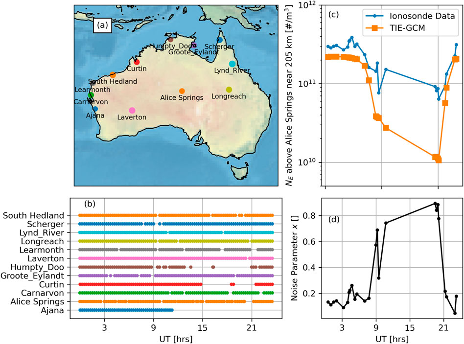
Figure 1. Ionosonde locations (A) and times (B). Electron density from the Alice Springs ionosonde and interpolated TIE-GCM electron density (C). See text for definition of noise parameter (D).

For each profile, we discard measurements that are not in the frequency or height range that is directly measured by the ionosonde. For example, even in these hand-scaled profiles, there is data extending above hmF2 which is model-driven. To remove points like this, we identify all measurements with electron densities lower than the maximum electron density at lower altitudes and delete them. This removes the topside and valley region. We also remove measurements below the minimum frequency actively measured by the ionosonde. This removes most low-altitude measurements during local night when the E region disappears.

Our goal with this work is to capture deviations from a smooth background. We use a Thermosphere-Ionosphere-Electrodynamics General Circulation Model (TIE-GCM) Richmond et al. (1992); Roble et al. (1977) run for the same day performed by the Community Coordinated Modeling Center (CCMC) as a background model for its accessibility and reproducibility. This background model has a native 2.5° resolution and 20 min timestep. We interpolate the electron density from the background model to the precise latitude, longitude, altitude, and time of each measurement. This is shown in Figure 1C which shows the electron density as a function of time for both the Alice Springs ionosonde in blue and the TIE-GCM electron density interpolated to the same location and time. We use measurements near 205 km here, knowing that the actual measurement altitude varies with each profile. Note the large gap in measurements at local night, and contrast the smoothness of the TIE-GCM electron density with the variability of the ionosonde measurements. To quantify the deviations from the smooth TIE-GCM background we use the noise parameter $x$ defined in Equation 1 to follow Hughes et al. (2022):

$x={\text{Log}}_{10}\left(N_{eI}\right)-{\text{Log}}_{10}\left(N_{eB}\right)(1)$

where $N_{eI}$ is the ionosonde measurement, and $N_{eB}$ is the smooth background, both in [#/${\mathrm{m}}^3$]. Since a log axis is used for Figure 1C, $x$ is the distance between the blue and orange lines. For this ionosonde and altitude, $x$ is positive all day, but when considering all ionosondes and altitudes $x$ is well-modeled by a Gaussian distribution with $\mu =0.26$ and $\sigma =0.28$. The sign of $\mu$ indicates that the real measurements are on average higher than TIE-GCM by a factor of $10^{0.26}\approx 1.82$ on this day and in this region.

In summary, our dataset contains 1,097 ionograms from 12 unique ionosondes. Each ionogram contains an electron density profile with many measurements of electron density. Each measurement in the region directly measured by the ionosonde is compared to the electron density from a TIE-GCM model run to compute $x$. In total, this results in 14,039 measurements of $x$ all at different latitudes, longitudes, altitudes, and times.

2.2 TEC data

The TEC data is the line-of-sight TEC data product publicly available from the Madrigal Database cos (Author Anonymous, 2019). This global data product is derived from GPS and GLONASS observations from more than 6,000 GNSS receivers, including about 60 in Australia that are used for this study. The line-of-sight TEC values along the raypaths from each receiver to the multiple GNSS satellites in view are reported at a 30 s cadence. The data product also includes the vertical TEC for each line-of-sight TEC value, calculated using a mapping function and placing the ionospheric piercing point (IPP) at 350 km altitude. For each station in the vicinity of Australia, we store the transmitting satellite, time, vertical TEC, and location of the IPP.

The vertical TEC data are further processed in a manner similar to Azeem et al. (2017). This study detrended the TEC by subtracting a running 40 min mean to yield dTEC. This detrending would remove the long-period TIDs which we wish to study in this analysis, so we do not detrend our TEC. Portions of the TEC arc with the GNSS satellite elevation angle below $20°$ are discarded. Figure 2 shows the density of the Madrigal data.

Figure 2

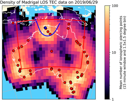
Figure 2. Density of Madrigal TEC data in the vicinity of Australia on 2019/06/29. The blue dot on the map is the location of an exemplary receiver (01na) and the blue line is the IPP track for an example TEC arc (GPS PRN 21).

The TEC data are then binned into 15 min in time and $1.5°\times 1.5°$ in latitude and longitude, within a geographical boundary of $[-31°,8.5°]$ latitude and $[117°,150°]$ longitude (the red boundary in Figure 2). This boundary is chosen to approximately match the geographical extent of ionosondes shown in Figure 1A. There are some gaps in the binned data due to the irregular distribution of IPP locations. For each time bin, the gaps in latitude and longitude bins are filled using 2D linear interpolation. No extrapolation is necessary for the chosen geographical boundary.

3 Methods

3.1 ND LSP

Many different methods have been used to study periodic structures in the ionosphere. If the data are regularly spaced, Fourier analysis using the Fast Fourier Transform (FFT) provides robust and easily interpretable results. Furthermore, FFT analysis is supported in virtually every scientific computing language making it readily available. If the data are not regularly spaced, they can be interpolated onto a regular grid, but this can affect the spectra depending on the size of the gap being interpolated through Munteanu et al. (2016). Techniques that do not require interpolation include phase folding, least squares, and Bayesian methods. One very powerful member of the least squares family of spectral analysis techniques is the Lomb-Scargle Periodogram (LSP) named for Lomb (1976) and Scargle (1982). This technique is very common in astronomy and astrophysics where measurements are typically irregular. An excellent review of this technique and its use can be found in VanderPlas (2018). The 1D LSP is a well-studied numerical technique Press et al. (1992) and is supported in many common scientific programming languages such as Matlab, Python, and IDL. However, to the author’s knowledge, there is only one multivariate (N-D) implementation Seilmayer et al. (2022), and it is in the R programming language.¹ This is in contrast to Fourier analysis which has broad support for N-dimensional analysis. Their derivation is briefly repeated here. We have implemented this in python, with a broadcasting extension. The python package as well as a demo and visualization script are provided on github.

3.1.1 Derivation

Assume that we have a dependent variable $y$ that is a function of $L$ different independent variables which we group into the vector $\vec{X}$. For our case, $y$ is the electron density, which is a function of the four independent variables of time, altitude, latitude, and longitude, so $\vec{X}={[t,a,\text{lat},\text{lon}]}^T$. Further, assume that we have $n$ samples of our independent and dependent variables so that $y$ is of shape $[n]$ and $X$ is of shape [$L$, $n$). Assuming that our signal is periodic, we are interested in finding the coefficients $a_k$ and $b_k$ in a spectral decomposition defined in Equation 2:

$y\left(\vec{X}\right)={\displaystyle \sum _{k=0}^M}{a}_k\cos \left({\vec{\omega }}_k\cdot \left(\vec{X}-{\vec{\tau }}_k\right)\right)+b_k\sin \left({\vec{\omega }}_k\cdot \left(\vec{X}-{\vec{\tau }}_k\right)\right)(2)$

where each ${\vec{\omega }}_k$ is a size $[L]$ vector containing a unique set of frequencies. For our case, they are all of the form $[1/P,1/{\lambda }_z,1/{\lambda }_{\text{Lat}},1/{\lambda }_{\text{Lon}}]$ for periods $P$ and wavelengths $\lambda$. The coefficients $a_k,b_k$, describe the amplitude and phase of $y$ at frequency ${\vec{\omega }}_k$. Equation 2 differs from the standard discrete Fourier decomposition in two ways; first, the frequencies ${\vec{\omega }}_k$ are not a priori fixed; and second, the parameters ${\vec{\tau }}_k$ are frequency dependent. These differences cause the basis functions in the decomposition of Equation 2 to be not necessarily orthogonal. Hence, the calculation of such a decomposition requires a method to choose the parameters ${\vec{\omega }}_k$ and ${\vec{\tau }}_k$, preferably such that each of $\cos ({\vec{\omega }}_k\cdot (\vec{X}-{\vec{\tau }}_k))$, $\sin ({\vec{\omega }}_k\cdot (\vec{X}-{\vec{\tau }}_k))$, $\cos ({\vec{\omega }}_l\cdot (\vec{X}-{\vec{\tau }}_l))$, and $\sin ({\vec{\omega }}_l\cdot (\vec{X}-{\vec{\tau }}_l))$ are pairwise orthogonal for each $k\ne l$. Therefore, instead of computing the full decomposition, we calculate the parameter ${\vec{\tau }}_k$ such that the two functions $\cos ({\vec{\omega }}_k\cdot (\vec{X}-{\vec{\tau }}_k))$ and $\sin ({\vec{\omega }}_k\cdot (\vec{X}-{\vec{\tau }}_k))$ are orthogonal on our grid of observations, and subsequently project our observations onto these functions for a dense grid of choices for ${\vec{\omega }}_k$.

We ensure orthogonality by first defining a new parameter ${\tau }_k^{*}={\vec{\omega }}_k\cdot {\vec{\tau }}_k$ which we note is a scalar for each $k$. We must find the value of ${\tau }_k^{*}$ such that the sine and cosine term are orthogonal for our sampling, This leads to Equation 3:

${\displaystyle \sum _n}\sin \left({\vec{\omega }}_k\cdot {\vec{X}}_n-{\tau }_k^{*}\right)\cos \left({\vec{\omega }}_k\cdot {\vec{X}}_n-{\tau }_k^{*}\right)=0(3)$

Trigonometric identities are applied to render this equation only in sines and cosines of either ${\vec{\omega }}_k\cdot {\vec{X}}_n$ or ${\tau }_k^{*}$. Our goal is to isolate and solve for ${\tau }_k^{*}$. This results in Equation 4

${\displaystyle \sum _n}\left(\cos \left({\vec{\omega }}_k\cdot {\vec{X}}_n\right)\cos \left({\tau }_k^{*}\right)+\sin \left({\vec{\omega }}_k\cdot {\vec{X}}_n\right)\sin \left({\tau }_k^{*}\right)\right)\left(\sin \left({\vec{\omega }}_k\cdot {\vec{X}}_n\right)\cos \left({\tau }_k^{*}\right)-\cos \left({\vec{\omega }}_k\cdot {\vec{X}}_n\right)\sin \left({\tau }_k^{*}\right)\right)=0(4)$

After some algebraic manipulation, one can separate the ${\tau }_k^{*}$ in Equation 5:

$\tan \left(2{\tau }_k^{*}\right)=\frac{{\displaystyle \sum _n}\sin \left(2{\vec{\omega }}_k\cdot {\vec{X}}_n\right)}{{\displaystyle \sum _n}\cos \left(2{\vec{\omega }}_k\cdot {\vec{X}}_n\right)}(5)$

Where this sum is performed across each of the $n$ samples. Now that we have the value of ${\tau }_k^{*}$ that makes the sine and cosine terms orthogonal on our sampling domain, we can find the $a$ and $b$ parameters by taking the dot product with our dependent variable $y$This is done in Equation 6:

$a_k=\frac{{\displaystyle \sum _n}y\left({\vec{X}}_n\right)\cos \left({\vec{\omega }}_k\cdot {\vec{X}}_n-{\tau }_k^{*}\right)}{{\displaystyle \sum _n}\cos {\left({\vec{\omega }}_k\cdot {\vec{X}}_n-{\tau }_k^{*}\right)}^2}{b}_k=\frac{{\displaystyle \sum _n}y\left({\vec{X}}_n\right)\sin \left({\vec{\omega }}_k\cdot {\vec{X}}_n-{\tau }_k^{*}\right)}{{\displaystyle \sum _n}\sin {\left({\vec{\omega }}_k\cdot {\vec{t}}_n-{\tau }_k^{*}\right)}^2}(6)$

We can now find the amplitude $(A)$ and phase $(\varphi )$ of $y$ at the frequency ${\vec{\omega }}_k$ This is done in Equation 7:

$A_k=\sqrt{a_k^2+b_k^2}{\varphi }_k={\tan }^{-1}\left(b_k,a_k\right)(7)$

where the signs of $a_k,b_k$ must be used to determine the quadrant of the phase.

3.1.2 Frequency selection

Fourier and LSP analysis both assume that a wave is coherent over the domain. Since TIDs have wavelengths and periods that change with altitude e.g., Nicolls et al. (2004) the data are limited to altitudes above 150 km to minimize the effects of differing vertical wavelengths. TIDs change direction with time. For example, Crowley and Rodrigues (2012) showed that the prevailing TID direction is ${90}^{\text{o}}$ offset from the prevailing neutral wind direction which rotates through ${360}^{\text{o}}$ per day. If we used the full day of data simultaneously, TIDs of different azimuths might cancel out and not appear in the analysis. To minimize these types of errors, we only use data from 15 to 21 UT (1-7 LT) to focus on a particularly active time when the TIDs can be assumed to be more coherent. This time range also means that all measurements considered occur during local night. We apply the LSP to a subset of the ionosonde dataset by providing one-dimensional arrays of $N$, $E$, altitude, time, and the noise parameter $x$. The variables $N,E$ are the North and East distance (in km) from a central point at (−${20}^{\text{o}}$, ${130}^{\text{o}}$) in the center of Australia.

In Fourier analysis, the observable frequencies are given by Nyquist criterion. For LSP analysis, the frequencies must be chosen by the user. In general, uneven sampling allows for much higher frequencies to be resolved than any “pseudo-Nyquist” limits would indicate VanderPlas (2018). In fact, Eyer and Bartholdi (1999) shows that the theoretical maximum frequency is set by the number of significant digits in the data rather than the spacing. Instead of using these pseudo-Nyquist frequencies, we choose frequencies based on the TIDs that we hope to observe, and then use a shuffling approach to determine observability and significance. The periods for each dimension are shown in Table 1. Negative values for the spatial dimensions indicate motion in the opposite direction. For example, a −300 km northward period indicates a wave traveling south with a 300 km wavelength.

Table 1

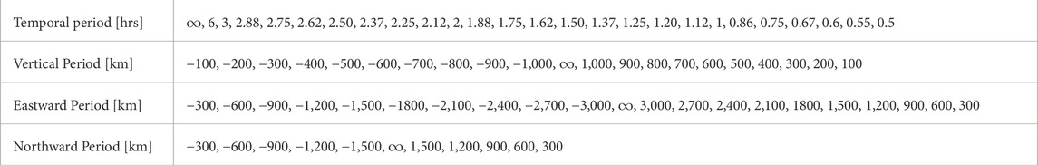
Table 1. Periods probed by LSP analysis.

We probe up to 1,000 km vertical wavelengths, despite only having measurements from $\sim$150 to $\sim$ 350 km. These long wavelengths would not be resolvable in only one dimension, as the vertical range is too short to see an entire period. However, we are able to discern these waves if they have a resolvable period in another dimension. For example, in van de Kamp et al. (2014), one can visually extrapolate where the constant phase contour would intersect the $y$ axis in their Figure 2 or 8.

To assess the significance of the amplitude, we empirically calculate the noise amplitude by shuffling the $x$ variable and re-running the ND LSP. We do this 10 times and average the two highest amplitudes for every combination of frequencies. This estimates the 95% significance threshold—amplitudes higher than this from the unshuffled data have less than a 5% probability of occurring simply due to the structure of the frequency grid and likely have physical significance. We also refer to the 95% significance threshold as the “noise amplitude”.

3.2 FFT TEC analysis

FFT analysis is applied to the binned dTEC data to identify periodic structures. As previously mentioned, the observable frequencies in Fourier analysis are set by the Nyquist criterion that depends on the sampling rate. The grid for binning dTEC was chosen to make the largest observable frequencies (equivalently, shortest observable period or wavelength) similar to those probed by the ND LSP of the ionosonde data. For the FFT analysis, the shortest period is 30 min and the shortest horizontal wavelength is 3° (approximately 330 km). Of course, the FFT analysis of the dTEC data cannot provide any information about the vertical frequencies that the ND LSP can reveal in the ionosonde data.

The amplitudes at frequencies $f_t$, $f_{\mathit{lon}}$, and $f_{\mathit{lat}}$ are determined by applying a 3D FFT (scipy.fft.fftn) to the binned dTEC data. The spatial frequencies in latitude and longitude in units of [1/degree] are converted to units of [1/km] using approximations $f_x=f_{\mathit{lon}}/\left(111\times \cos 20°\right)$ and $f_y=f_{\mathit{lat}}/111$. Our procedure for determining the 95% significance threshold is similar to the ND LSP. The 3D FFT is applied to 100 shuffled versions of the binned dTEC data and the 95th percentile for each point in frequency space is the significance threshold. We note that the shuffling is applied amongst the binned dTEC data prior to the 2D linear interpolation step, leaving the gaps in the same place. This ensures that the locations and times of the gaps (which occur more often in the interior of Australia where there are fewer IPP tracks) and their impact on the FFT results are properly accounted for in the 95% significance threshold.

4 Analysis

The spectra of the ionosonde and TEC data are four and three-dimensional, respectively, which makes visualization difficult. However, higher-dimensional datasets can be visualized by taking planar slices through a central point. For example, a 3-dimensional dataset $A=f(x,y,z)$ can be visualized by taking three orthogonal planar slices through a central point $(x_0,y_0,z_0)$ as $A_1=f(x_0,y,z),A_2=f(x,y_0,z),A_3=f(x,y,z_0)$. We use this approach to visualize the four-dimensional amplitude of the ionosonde data as a function of wavelength and period. While there are three orthogonal slices through a 3D dataset, there are six orthogonal planes that slice the four-dimensional amplitude array for the ionosonde data. In Figure 3, we show these six orthogonal slices for a central point corresponding to a TID moving northwest with a wavelength of ${\left(\sqrt{1/\mathrm{2,40}{0}^2+1/\mathrm{1,20}{0}^2}\right)}^{-1}\approx \mathrm{1,073}$ km and a period of 2.4 h. This wave has the highest amplitude of any of the significant waves with an amplitude more than twice the noise amplitude at this frequency. The amplitude of this wave is $\sim$0.12, which corresponds to variations in electron density on the order of $10^{0.12}-1=32\%$ compared to the smooth background.

Figure 3

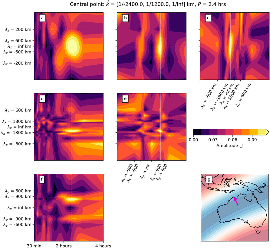
Figure 3. Panels (A–F) show six orthogonal slices through a four-dimensional ND LSP array through a central point. Panel (G) shows the wave that this central point corresponds to, with a magenta arrow showing the distance the wave moves in 1 h. See text for details.

Each panel shows a slice through a different plane. The central point is identified by the pair of thin white lines forming a crosshair in each panel. Panel (g) shows a map with the wave at this central point overlaid as color. The arrow shows the distance the wave travels in 1 h. This central point is a clear peak in panels (a–f), although it is more prominent in some dimensions than others. For example, panel (a) shows only two peaks, the central point being much higher than the secondary one while panel (e) shows a rich sea of other local peaks corresponding to horizontal waves with the same period but other azimuths and wavelengths.

Next, we apply a two-part threshold to identify significant waves and characterize them statistically. First, the amplitude must be larger than its neighbors in all dimensions. Points on the edge of the domain (such as temporal periods of 30 min or $\infty$) are not included, as one cannot know whether they are indeed a local max. Second, the amplitude must be larger than the empirically determined noise amplitude. This classifies 110 of the 126,126 points (0.087%) as statistically significant waves.

These 110 points are classified as either horizontal or non-horizontal waves. This binary distinction is based on a gap in the measured elevation angles. An elevation angle of 0 means that the TID propagates horizontally, and an elevation angle of 90 means the TID propagates vertically. Defining $k_h=\sqrt{k_x^2+k_y^2}$ and ${\lambda }_h=1/k_h$, the elevation angle is defined in Equation 8:

$e=\text{arctan}\left(k_z/k_h\right)=\text{arctan}\left({\lambda }_h/{\lambda }_z\right)(8)$

Horizontal waves $({\lambda }_z=\infty ,e=0)$ are observable, but the next lowest elevation wave comes from the largest vertical wavelength (${\lambda }_z=\mathrm{1,000}$ km) and the shortest horizontal wavelength (${\lambda }_h=1/\sqrt{1/300^2+1/300^2}\approx 212$ km). This gives an elevation angle of arctan (0.212) $\approx 12^{\text{o}}$. Therefore, waves with $e=0$ are classified as horizontal and all others are classified as non-horizontal. The periods, wavelengths, elevations, and travel directions are shown in Figure 4.

Figure 4

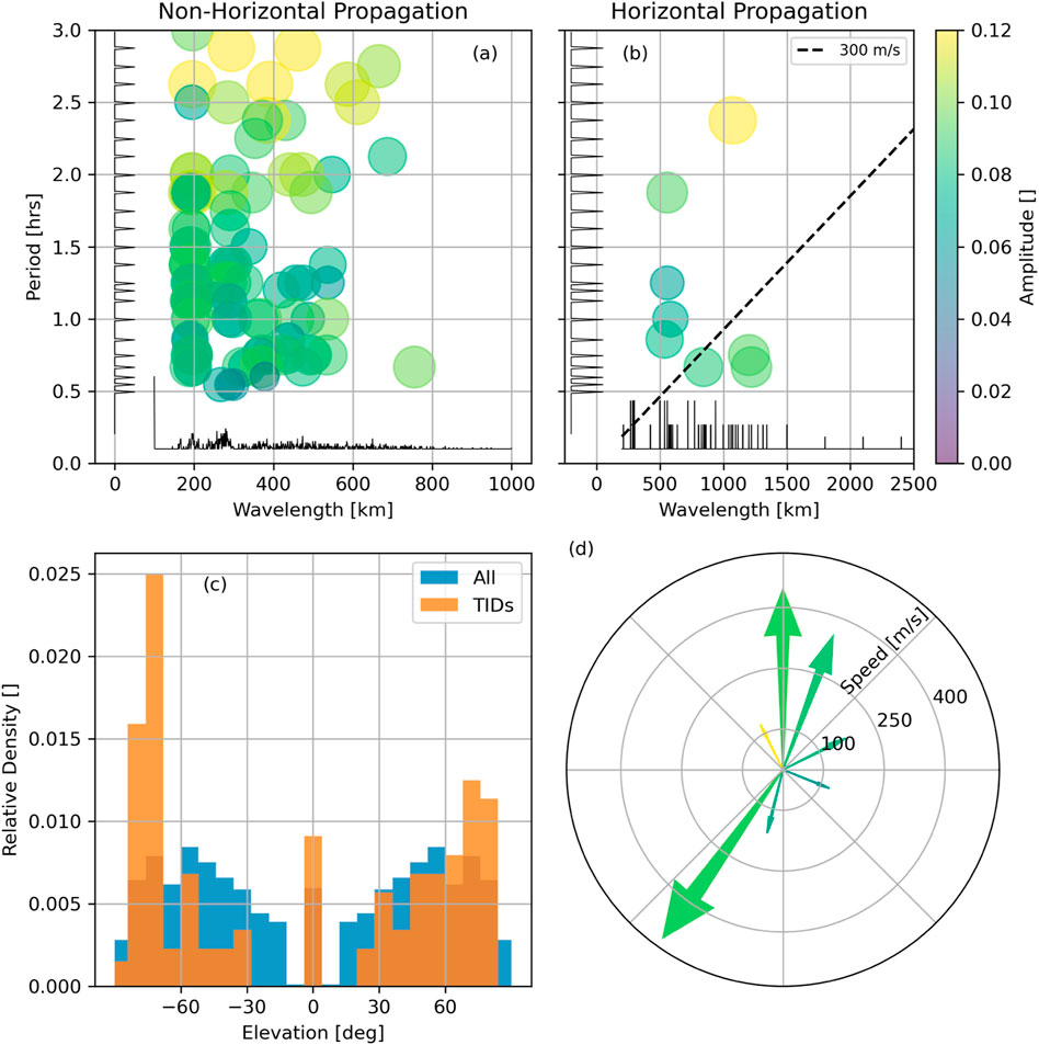
Figure 4. Waves with non-horizontal propagation are characterized in the left column and waves with horizontal propagation are characterized in the right column. Panels (A, B) show scatter plots with the wavelength, period, and amplitude. Panel (C) shows a normalized histogram of the elevation angles for both TIDs and all measured points. Panel (D) shows the speed as a function of azimuth for the horizontal waves. In panels (A, B, D), color indicates the amplitude of the wave.

Panel (a) of Figure 4 shows a scatter plot of the period and wavelength for the non-horizontal waves. The color and size of the dots indicate the amplitude of the waves. A typical amplitude is 0.075 which translates to a $10^{0.075}\approx 19\%$ amplitude deviation in electron density. Thin black lines on both margins show normalized histograms of the wavelengths and periods measured. These histograms aid interpretation by showing whether the lack of a scatter point indicates that there was no TID with those characteristics in the ionosphere, or whether that wavelength and period were simply not probed. Panel (c) shows a normalized histogram of the elevation angle for all 126,126 points (blue) and the 110 TIDs (orange). The blue histogram shows the gaps between 0 and $\pm 12^{\text{o}}$ as well as a preference for angles near ${50}^{\text{o}}$. The difference between the shape of the orange and blue distribution shows that TIDs are most common near ${70}^{\text{o}}$ elevation angles. There is an asymmetry in the distribution with $-70^{\text{o}}$ elevation angles being much more common than $+70^{\text{o}}$ elevation angles, suggesting that on this day more waves originated from above than from below. Additionally, the lowest elevation angle for TIDs is $\sim 23^{\text{o}}$ despite frequencies leading to lower elevation angles being measured which indicates a real absence rather than a lack of measurement.

There are many more non-horizontal waves than horizontal ones. The period and wavelength of the eight horizontal waves are shown in Figure 4B. The black dashed line shows a speed of 300 m/s. Points to the left of this line have speeds $>$ 300 m/s, and points to the right have speeds $<$ 300 m/s. Figure 4D shows the speed as a function of azimuth for the horizontal waves.

Our instrument geometry and cadence as well as the frequencies probed preclude observation of some waves. We have previously discussed the limitations in elevation angle, but our 15 min measurement cadence and corresponding 30 min minimum resolvable period prevents all acoustic waves and many small-scale and medium-scale TIDs from being measured. We also lack the ability to resolve short horizontal wavelength waves. Even with these limitations, we can still comment on the amount of variance that is explained by waves in the probed frequency domain. We do this by summing the amplitudes of all 110 of the significant waves, and comparing this to the sum of the amplitudes at all probed frequencies. This indicates that waves account for approximately 0.157% of the total deviation from a smooth background.

Now we compare the results of the ionosonde ND LSP analysis to the TEC analysis for the horizontal waves. Figure 5 shows a scatter plot of the waves found using the TEC data as large colored circles. The size and color of the circle indicate the amplitude of the waves in TECU. Thin black lines in the margins show the measured wavelengths and periods in the TEC data. The black dashed line shows a speed of 300 m/s, just as in Figure 4. Additionally, this plot shows red x markers for the eight significant horizontal TIDs from the LSP analysis of the ionosonde data.

Figure 5

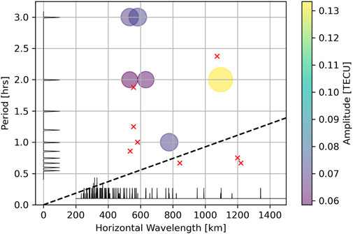
Figure 5. Scatter plot of period vs. wavelength for horizontal waves using TEC data and FFT analysis. Small red “x” symbols indicate the horizontal TIDs found using ionosonde data and ND LSP analysis and shown in Figure 4B.

Because the measured periods and wavelengths are slightly different, we do not see exact matches for the waves found using each dataset/method. However, the largest TID in both analyses is very similar, having a period and wavelength of (2.4 h, 1,073 km) in the ND LSP analysis and (2 h, 1,095 km) in the TEC FFT analysis. Because the FFT analysis does not oversample the frequencies, it is possible that the peak at 2 h is the shoulder of a peak that is truly closer to 2.4 h. There are two TIDs in the TEC analysis near (3 h, 600 km) that do not have a match in the ionosonde ND LSP analysis. However, there is another pair near (2 h, 600 km) that do match a single ionosonde ND LSP TID. There is a single TEC TID near (1 h period, 800 km) that is near an ND LSP TID with a slightly lower period and slightly longer wavelength. There are two clusters of ND LSP TIDs near (45 min, 1,200 km) and (1 h, 550 km) that do not have corresponding TEC TIDs. In total, there are three close matches (2 h, 1,100 km), (2 h, 600 km), (1 h, 800 km) of which the first is the strongest TID in either analysis. There are two clusters in the ND LSP analysis (45 min, 1,200 km), (1 h, 600 km) with no match from the TEC analysis. There is one cluster in the TEC analysis (3 h, 600 km) that has no match on the ND LSP ionosonde analysis.

Perhaps the most likely reason for these discrepancies is that we are measuring the TEC signatures of non-horizontal TIDs. A full mapping of amplitude and elevation angle to the TEC signature would require topside densities which are not measured in the ionosonde data used here. However, we can say that near horizontal TIDs with the vertical wavelength ${\lambda }_z$ greater than the “thickness” of the ionosphere ($\sim$500 km) which contributes significant TEC, will impact vertical TEC measurements. More specifically, a vertical ray has no chance of cancellation by traveling through a peak and trough. Smaller ${\lambda }_z$ values may also affect vertical TEC measurements, but cancellation will muddle their interpretation. We use a minimum TEC elevation angle of ${20}^{\text{o}}$ in this work which could lead to complex aliasing of these non-horizontal TIDs and could explain why there are TIDs present in the TEC analysis absent from the ionosonde ND LSP horizontal analysis.

5 Discussion

Comparing the ND LSP results to previous observations, we see general agreement in vertical TID characteristics. Although most TID observations focus only on horizontal characteristics, ISR observations have previously been used to measure the vertical structure of TIDs. Shibata and Schlegel (1993) used EISCAT Tromso to study vertical and horizontal TID propagation. During a geomagnetically quiet period (9/7/1988), they found AGWs they observed AGWs with an average elevation angle of $71.5°$, consistent with the TID parameters observed in this study. Additionally, Chum et al. (2021) found a maximum elevation angle near $70°$ ($-30°$ in their coordinate system) for results collected over a year at solar min and solar max. The azimuthal angle of propagation was also similar to that of the largest amplitude waves found in the current study. Rice et al. (1988) examined TIDs using multiple ISRs during the WAGS campaign (10/18/1985, moderate geomagnetic activity) and observed TIDs with elevation angles 75.5–82 $°$.

These results also show overall agreement with previous studies on TID propagation and horizontal characteristics. The observed horizontal TIDs have speeds from 100–400 m/s. These speeds are slower than average LSTID speeds Hocke and Schlegel (1996), Hajkowicz (1991), but are within the expected range of speeds. The largest observed TID in this analysis had a period of 2.4 h. Similar TIDS with a dominant mode of 2.5–3.5 h have been observed in the southern hemisphere Habarulema et al. (2013).

The LSP technique is novel in that it can examine both horizontal and vertical propagation of TIDs using ionosonde data. Most observational studies have only examined horizontal propagation. Characterizing both vertical and horizontal propagation gives a more accurate picture of TID dynamics.

6 Conclusions and future work

In this paper, we have used a N-dimensional Lomb Scargle Periodogram and demonstrated its utility on a dataset consisting of high-cadence ionograms with minimal processing and no interpolation. The resulting analysis is compared to a concurrent analysis of line of sight TEC data. The two analyses agree on the horizontally-propagating TIDs which are resolvable by both methods. The ionosonde LSP analysis additionally resolves a spectrum of propagation elevation angles. The ND LSP is a complementary technique to other spectral analysis methods that can resolve periodic structures from unstructured data. Although shown here for ionosonde data, the ND LSP could be applied to TEC data as well.

We show for this dataset that TIDs are more common at $\sim {70}^{\text{o}}$ than other elevation angles. Although this population of near-vertical TIDs has been observed before, it has received much less study than its horizontal counterpart. This population can easily be mischaracterized or completely lost if using TEC data with the thin-shell approximation.

Future work has many possible avenues. First, this technique could be used with ionosonde data for active periods with known TIDs such as tsunamis, large convective storms, and geomagnetically active periods where the aurora launches TIDs equatorward. Secondly, this technique could be used with dispersed space in-situ data such as mIVM measurements from COSMIC-2 and other missions.

7 Appendix

The code for computing the ND LSP on general data is provided here https://github.com/joe-hughes26/ND-LSP along with a demo script and visualization.

Data availability statement

Publicly available datasets were analyzed in this study. Simulation results for the TIE-GCM run have been provided by the Community Coordinated Modeling Center (CCMC) at Goddard Space Flight Center through their publicly available simulation services https://ccmc.gsfc.nasa.gov. The specific run is hosted at https://ccmc.gsfc.nasa.gov/results/viewrun.php?domain&equals;IT&runnumber&equals;Joe_Hughes_050423_IT_1.

Author contributions

JH: Conceptualization, Investigation, Methodology, Software, Visualization, Writing–original draft. IC: Data curation, Formal Analysis, Methodology, Software, Validation, Visualization, Writing–original draft. AN: Methodology, Validation, Visualization, Writing–review and editing. RK: Software, Writing–review and editing. WW: Funding acquisition, Project administration, Resources, Supervision, Writing–review and editing. KO: Funding acquisition, Project administration, Resources, Writing–review and editing. RL: Funding acquisition, Project administration, Resources, Supervision, Writing–review and editing. JC: Funding acquisition, Project administration, Resources, Supervision, Writing–review and editing. JM: Funding acquisition, Project administration, Resources, Writing–review and editing.

Funding

The author(s) declare that financial support was received for the research, authorship, and/or publication of this article. This work was performed as part of the Impact of Ionospheric Irregularities program at AFRL/RVB under the leadership of KO on contract FA9453-19-C-0400.

Acknowledgments

The authors extend many thanks to Federico Gasperini, Jeff Steward, and Ryan Nguyen for many fruitful discussions on the ND LSP. We thank the Defense Science and Technology Group (DSTG) for providing the ionosonde data. The views expressed are those of the authors and do not reflect the official guidance or position of the United States Government, the Department of Defense or of the United States Air Force. The appearance of external hyperlinks does not constitute endorsement by the United States Department of Defense (DoD) of the linked websites, or the information, products, or services contained therein. The DoD does not exercise any editorial, security, or other control over the information you may find at these locations.

Conflict of interest

Authors JH, IC, AN, RK and WW were employed by Orion Space Solutions.

The remaining authors declare that the research was conducted in the absence of any commercial or financial relationships that could be construed as a potential conflict of interest.

Generative AI statement

The author(s) declare that no Generative AI was used in the creation of this manuscript.

Publisher’s note

All claims expressed in this article are solely those of the authors and do not necessarily represent those of their affiliated organizations, or those of the publisher, the editors and the reviewers. Any product that may be evaluated in this article, or claim that may be made by its manufacturer, is not guaranteed or endorsed by the publisher.

Footnotes

¹https://cran.r-project.org/web/packages/spectral/spectral.pdf

References

Author Anonymous (2019). Data from the cedar madrigal database.

Google Scholar

Azeem, I., Vadas, S. L., Crowley, G., and Makela, J. J. (2017). Traveling ionospheric disturbances over the United States induced by gravity waves from the 2011 tohoku tsunami and comparison with gravity wave dissipative theory. J. Geophys. Res. Space Phys. 122, 3430–3447. doi:10.1002/2016JA023659

CrossRef Full Text | Google Scholar

Azeem, I., Walterscheid, R. L., and Crowley, G. (2018). Investigation of acoustic waves in the ionosphere generated by a deep convection system using distributed networks of gps receivers and numerical modeling. Geophys. Res. Lett. 45, 8014–8021. doi:10.1029/2018GL078107

CrossRef Full Text | Google Scholar

Azeem, I., Yue, J., Hoffmann, L., Miller, S. D., Straka, W. C., and Crowley, G. (2015). Multisensor profiling of a concentric gravity wave event propagating from the troposphere to the ionosphere. Geophys. Res. Lett. 42, 7874–7880. doi:10.1002/2015GL065903

CrossRef Full Text | Google Scholar

Becker, E., and Vadas, S. L. (2018). Secondary gravity waves in the winter mesosphere: results from a high-resolution global circulation model. J. Geophys. Res. Atmos. 123, 2605–2627. doi:10.1002/2017JD027460

CrossRef Full Text | Google Scholar

Becker, E., Vadas, S. L., Bossert, K., Harvey, V. L., Zülicke, C., and Hoffmann, L. (2022). A high-resolution whole-atmosphere model with resolved gravity waves and specified large-scale dynamics in the troposphere and stratosphere. J. Geophys. Res. Atmos. 127, e2021JD035018. doi:10.1029/2021jd035018

CrossRef Full Text | Google Scholar

Chou, M.-Y., Lin, C. C. H., Shen, M.-H., Yue, J., Huba, J. D., and Chen, C.-H. (2018). Ionospheric disturbances triggered by spacex falcon heavy. Geophys. Res. Lett. 45, 6334–6342. doi:10.1029/2018GL078088

CrossRef Full Text | Google Scholar

Chum, J., Podolska, K., Rusz, J., Base, J., and Tedoradze, N. (2021). Statistical investigation of gravity wave characteristics in the ionosphere. Earth, Planets, Space 73, 60. doi:10.1186/s40623-021-01379-3

CrossRef Full Text | Google Scholar

Crowley, G., Azeem, I., Reynolds, A., Duly, T. M., McBride, P., Winkler, C., et al. (2016). Analysis of traveling ionospheric disturbances (tids) in gps tec launched by the 2011 tohoku earthquake. AGU Radio Sci. 51, 507–514. doi:10.1002/2015RS005907

CrossRef Full Text | Google Scholar

Crowley, G., and Rodrigues, F. S. (2012). Characteristics of traveling ionospheric disturbances observed by the tiddbit sounder. Radio Sci. 47. doi:10.1029/2011RS004959

CrossRef Full Text | Google Scholar

Emmons, D. J., Dao, E. V., Knippling, K. K., McNamara, L. F., Nava, O. A., Obenberger, K. S., et al. (2020). Estimating horizontal phase speeds of a traveling ionospheric disturbance from digisonde single site vertical ionograms. Radio Sci. 55, e2020RS007089. doi:10.1029/2020RS007089

CrossRef Full Text | Google Scholar

Eyer, L., and Bartholdi, P. (1999). Variable stars: which nyquist frequency? Astron. Astrophys. Suppl. Ser. 135, 1–3. doi:10.1051/aas:1999102

CrossRef Full Text | Google Scholar

Frissell, N. A., Baker, J., Ruohoniemi, J. M., Gerrard, A. J., Miller, E. S., Marini, J. P., et al. (2014). Climatology of medium-scale traveling ionospheric disturbances observed by the midlatitude blackstone superdarn radar. J. Geophys. Res. Space Phys. 119, 7679–7697. doi:10.1002/2014JA019870

CrossRef Full Text | Google Scholar

Galkin, I., and Reinsch, B. (2008). “The new artist 5 for all digisondes,” in Ionosonde Network advisory group bulletin (Sydney, New South Wales, Austrailia).

Google Scholar

Gong, Y., Lv, X., Zhang, S., Zhou, Q., and Ma, Z. (2021). Climatology and seasonal variation of the thermospheric tides and their response to solar activities over arecibo. J. Atmos. Solar-Terrestrial Phys. 215, 105592. doi:10.1016/j.jastp.2021.105592

CrossRef Full Text | Google Scholar

Gong, Y., Xue, J., Ma, Z., Zhang, S., Zhou, Q., Huang, C., et al. (2022). Observations of a strong intraseasonal oscillation in the mlt region during the 2015/2016 winter over mohe, China. J. Geophys. Res. Space Phys. 127, e2021JA030076. doi:10.1029/2021JA030076

CrossRef Full Text | Google Scholar

Gong, Y., Zhou, Q., and Zhang, S. (2013). Atmospheric tides in the low-latitude e and f regions and their responses to a sudden stratospheric warming event in january 2010. J. Geophys. Res. Space Phys. 118, 7913–7927. doi:10.1002/2013JA019248

CrossRef Full Text | Google Scholar

Goodwin, L. V., and Perry, G. W. (2022). Resolving the high-latitude ionospheric irregularity spectra using multi-point incoherent scatter radar measurements. Radio Sci. 57, e2022RS007475. doi:10.1029/2022RS007475

CrossRef Full Text | Google Scholar

Habarulema, J. B., Katamzi, Z. T., and McKinnell, L.-A. (2013). Estimating the propagation characteristics of large-scale traveling ionospheric disturbances using ground-based and satellite data. J. Geophys. Res. Space Phys. 118, 7768–7782. doi:10.1002/2013JA018997

CrossRef Full Text | Google Scholar

Hajkowicz, L. A. (1991). Auroral electrojet effect on the global occurrence pattern of large scale travelling ionospheric disturbances. Planet. Space Sci. 39, 1189–1196. doi:10.1016/0032-0633(91)90170-F

CrossRef Full Text | Google Scholar

Harris, T. J., Cervera, M. A., and Meehan, D. H. (2012). Spice: a program to study small-scale disturbances in the ionosphere. J. Geophys. Res. Space Phys. 117. doi:10.1029/2011JA017438

CrossRef Full Text | Google Scholar

Harris, T. J., Quinn, A. D., and Pederick, L. H. (2016). The dst group ionospheric sounder replacement for jorn. Radio Sci. 51, 563–572. doi:10.1002/2015RS005881

CrossRef Full Text | Google Scholar

Hocke, K., and Schlegel, K. (1996). A review of atmospheric gravity waves and travelling ionospheric disturbances: 1982-1995. Ann. Geophys. 14, 917–940. doi:10.1007/s00585-996-0917-6

CrossRef Full Text | Google Scholar

Huang, C. Y., Helmboldt, J. F., Park, J., Pedersen, T. R., and Willemann, R. (2019). Ionospheric detection of explosive events. Rev. Geophys. 57, 78–105. doi:10.1029/2017RG000594

CrossRef Full Text | Google Scholar

Hughes, J., Forsythe, V., Blay, R., Azeem, I., Crowley, G., Wilson, J., et al. (2022). On constructing a realistic truth model using ionosonde data for observation system simulation experiments. AGU Radio Sci. 57. doi:10.1029/2022RS007508

CrossRef Full Text | Google Scholar

Li, X., Ding, F., Yue, X., and Li, J. (2022). Short-period concentric traveling ionospheric disturbances excited by the launch of China’s long march 4b rocket detected by 1 hz gnss data. AGU Space Weather 20. doi:10.1029/2021SW003003

CrossRef Full Text | Google Scholar

Loi, S. T., Cairns, I. H., Murphy, T., Erickson, P. J., Bell, M. E., Rowlinson, A., et al. (2016). Density duct formation in the wake of a travelling ionospheric disturbance: murchison widefield array observations. J. Geophys. Res. Space Phys. 121, 1569–1586. doi:10.1002/2015JA022052

CrossRef Full Text | Google Scholar

Lomb, N. (1976). Least-squares frequency analysis of unequally spaced data. Astrophysics Space Sci. 39, 447–462. doi:10.1007/BF00648343

CrossRef Full Text | Google Scholar

Mabie, J., and Bullett, T. (2019). Infrasonic wave-induced variations of ionospheric hf sounding echoes. Radio Sci. 54, 876–887. doi:10.1029/2019RS006826

CrossRef Full Text | Google Scholar

Mabie, J., Bullett, T., Moore, P., and Vieira, G. (2016). Identification of rocket-induced acoustic waves in the ionosphere. Geophys. Res. Lett. 43, 11024–11029. doi:10.1002/2016GL070820

CrossRef Full Text | Google Scholar

Makela, J. J., and Otsuka, Y. (2012). Overview of nighttime ionospheric instabilities at low- and mid-latitudes: coupling aspects resulting in structuring at the mesoscale. Space Sci. Rev. 168, 419–440. doi:10.1007/s11214-011-9816-6

CrossRef Full Text | Google Scholar

Martinis, C., Baumgardner, J., Wroten, J., and Mendillo, M. (2011). All-sky imaging observations of conjugate medium-scale traveling ionospheric disturbances in the american sector. J. Geophys. Res. Space Phys. 116. doi:10.1029/2010JA016264

CrossRef Full Text | Google Scholar

Morgan, M. G., Calderón, C. H. J., and Ballard, K. A. (1978). Techniques for the study of tid’s with multi-station rapid-run ionosondes. Radio Sci. 13, 729–741. doi:10.1029/RS013i004p00729

CrossRef Full Text | Google Scholar

Munteanu, C., Negrea, C., Echmin, M., and Mursula, K. (2016). Effect of data gaps: comparison of different spectral analysis methods. Ann. Geophys. 34, 437–449. doi:10.5194/angeo-34-437-2016

CrossRef Full Text | Google Scholar

Nicolls, M. J., Kelley, M. C., Coster, A. J., González, S. A., and Makela, J. J. (2004). Imaging the structure of a large-scale tid using isr and tec data. Geophys. Res. Lett. 31. doi:10.1029/2004GL019797

CrossRef Full Text | Google Scholar

Nishioka, M., Tsugawa, T., Kubota, M., and Ishii, M. (2013). Concentric waves and short-period oscillations observed in the ionosphere after the 2013 moore ef5 tornado. Geophys. Res. Lett. 40, 5581–5586. doi:10.1002/2013GL057963

CrossRef Full Text | Google Scholar

Obenberger, K. S., Dao, E., and Dowell, J. (2019). Experimenting with frequency-and-angular sounding to characterize traveling ionospheric disturbances using the lwa-sv radio telescope and a dps4d. Radio Sci. 54, 181–193. doi:10.1029/2018RS006690

CrossRef Full Text | Google Scholar

Oinats, A., Kurkin, V., and Nishitani, N. (2015). Statistical study of medium-scale traveling ionospheric disturbances using superdarn hokkaido ground backscatter data for 2011. Earth Planets Space 67, 22. doi:10.1186/s40623-015-0192-4

CrossRef Full Text | Google Scholar

Otsuka, Y., Shinbori, A., Tsugawa, T., and Nishioka, M. (2021). Solar activity dependence of medium-scale traveling ionospheric disturbances using gps receivers in Japan. Earth, Planets Space 73, 22. doi:10.1186/s40623-020-01353-5

CrossRef Full Text | Google Scholar

Press, W. H., Teukolsky, S. A., Vetterling, W. T., and Flannery, B. P. (1992). Numerical recipies: the art of scientific computing. Cambridge University Press.

Google Scholar

Reinisch, B., Galkin, I., Belehaki, A., Paznukhov, V., Huang, X., Altadill, D., et al. (2018). Pilot ionosonde network for identification of traveling ionospheric disturbances. Radio Sci. 53, 365–378. doi:10.1002/2017RS006263

CrossRef Full Text | Google Scholar

Rice, D. D., Hunsucker, R. D., Lanzerotti, L. J., Crowley, G., Williams, P. J. S., Craven, J. D., et al. (1988). An observation of atmospheric gravity wave cause and effect during the october 1985 wags campaign. Radio Sci. 23, 919–930. doi:10.1029/RS023i006p00919

CrossRef Full Text | Google Scholar

Richmond, A. D., Ridley, E. C., and Roble, R. G. (1992). A thermosphere/ionosphere general circulation model with coupled electrodynamics. Geophys. Res. Lett. 6, 601–604. doi:10.1029/92gl00401

CrossRef Full Text | Google Scholar

Roble, R. G., Dickinson, R. E., and Ridley, E. C. (1977). Seasonal and solar cycle variations of the zonal mean circulation in the thermosphere. J. Geophys. Res. 82, 5493–5504. doi:10.1029/JA082i035p05493

CrossRef Full Text | Google Scholar

Sanchez, S., Kherani, E., Astafyeva, E., and de Paula, E. (2022). Ionospheric disturbances observed following the ridgecrest earthquake of 4 july 2019 in California, USA. Remote Sens. 14, 188. doi:10.3390/rs14010188

CrossRef Full Text | Google Scholar

Scargle, J. (1982). Studies in astronomical time series analysis ii. statistical aspects of spectral analysis of unevenly spaced data. Astrophysical J. 263, 835–853. doi:10.1086/160554

CrossRef Full Text | Google Scholar

Seilmayer, M., Gonzalez, F. G., and Wondrak, T. (2022). The multivariate extension of the lomb-scargle method. arXiv.

Google Scholar

Shibata, T., and Schlegel, K. (1993). Vertical structure of agw associated ionospheric fluctuations in the e- and lower f-region observed with eiscat-a case study. J. Atmos. Terr. Phys. 55, 739–749. doi:10.1016/0021-9169(93)90017-S

CrossRef Full Text | Google Scholar

Tedd, B. L., and Morgan, M. G. (1985). Tid observations at spaced geographic locations. J. Geophys. Res. Space Phys. 90, 12307–12319. doi:10.1029/JA090iA12p12307

CrossRef Full Text | Google Scholar

Vadas, S. L., and Azeem, I. (2021). Concentric secondary gravity waves in the thermosphere and ionosphere over the continental United States on march 25–26, 2015 from deep convection. J. Geophys. Res. Space Phys. 126. doi:10.1029/2020JA028275

CrossRef Full Text | Google Scholar

Vadas, S. L., and Crowley, G. (2010). Sources of the traveling ionospheric disturbances observed by the ionospheric tiddbit sounder near wallops island on 30 october 2007. J. Geophys. Res. Space Phys. 115. doi:10.1029/2009JA015053

CrossRef Full Text | Google Scholar

van de Kamp, M., Pokhotelov, D., and Kauristie, K. (2014). Tid characterised using joint effort of incoherent scatter radar and gps. Ann. Geophys. 32, 1511–1532. doi:10.5194/angeo-32-1511-2014

CrossRef Full Text | Google Scholar

VanderPlas, J. T. (2018). Understanding the lomb–scargle periodogram. Astrophysical J. Suppl. Ser. 236, 16. doi:10.3847/1538-4365/aab766

CrossRef Full Text | Google Scholar