The SDEMMA model for galactic cosmic ray and its dosimetric application

Introduction: Future crewed missions to Mars will encounter substantially elevated radiation levels compared to low Earth orbit operations. To address this challenge, we present the Space-Dependent Energetic cosmic ray Modulation using MAgnetic spectrometer (SDEMMA) model, a novel framework for modeling galactic cosmic ray (GCR) dynamics in deep-space environments.

Methods: The model employs stochastic differential equations with outer boundary conditions derived from contemporary local interstellar spectrum models. Time-dependent diffusion and drift coefficients were optimized through Markov Chain Monte Carlo parameter fitting against 2006-2019 observational data from the space-borne magnetic spectrometers of AMS-02 and PAMELA.

Results: SDEMMA extends GCR spectral calculations to radial positions beyond 1.0 AU, explicitly resolving radial gradients under diverse heliospheric conditions. The framework provides spatiotemporally resolved GCR spectra for charge numbers Z=1–28 at rigidities >0.2 GV, covering the inner heliosphere between Earth and Mars and currently the 2006-2019 epoch.

Discussion: Implementation demonstrates the model's operational utility: dose equivalent rates behind 30 g/cm² polyethylene shielding during a flux minimum range from 14-17 cSv/yr, with variance attributable to quality factor selection.

1 Introduction

While radiation exposure for astronauts in a low Earth orbit or even during a journey to the Moon can now be considered less challenging, this problem is still not well understood in the next natural step for a journey to the Mars. Due to the absence of the geomagnetic field shielding and a longer trip which last for years, the radiation level is much higher. Few in situ measurements have been performed. The Radiation Assessment Detector (RAD) on the Mars Science Laboratory (MSL), also known as the Curiosity rover, made the first-ever measurement during the transit from Earth to Mars in the 2011 Mars mission time window (Zeitlin et al., 2013). The total measured dose equivalent rate is $1.81\pm 0.33$ mSv/d. Analysis also shows that behind an average shielding of $16{\text{g/cm}}^2$, the galactic cosmic rays (GCR) made the dominant dose contribution in the energy range of $\sim 300$ MeV/n to $\sim 10$ GeV/n, while the solar energetic particles only contributed approximately $5\%$. Then the dose contribution of GCR is calculated by a rescaling of the MSL/RAD results under different solar modulation conditions in Guo et al. (2015). During the 2016 time window, a Liulin-MO dosimeter on the ExoMars Trace Gas Orbiter conducted a second measurement that was claimed to be consistent with the first MSL/RAD measurement (Semkova et al., 2018), given the modulation condition difference.

Such GCRs induced radiation dose in the transit orbit represents the most important radiation exposure during the human exploration of Mars (Guo et al., 2024), since GCRs are a continuous radiation source that is hard to shield against. On the other hand, the SEP events can be shielded in a better shelter part of a spacecraft for a few hours. And once on the planet, Mars’ atmosphere provides some protection, and a sub-surface shelter gives even more protection. Therefore, this important problem deserves further study. Without expensive in situ measurements, our goal is to develop a model-based calculation for the cumulative radiation dose experienced by astronauts on the journey to Mars (HelMod, 2024; Opher et al., 2023). This calculation scheme is aimed to (a) cover various possible Mars mission time windows under different solar modulation conditions, (b) provide full radial dependence, and (c) be applied to realistic target astronaut phantoms with flexible shielding. The goal involves researches in several broad field, and we plan to achieve it in a step by step manner. In the present paper we will mainly address the more “academic” GCR related issue (a and b), and keep the discussion of the space dosimetry (c) only at an illustrative level. The more realistic “engineering” dosimetric values will be provided in a forthcoming publication.

GCR spectra are influenced by solar activity, with the solar wind and interplanetary magnetic field playing crucial roles in their modulation. This variability with time is continuously captured by numerous experiments conducted on or around the Earth. Here, we use data in time series from space-borne magnetic spectrometers, specifically the PAMELA and the AMS-02 (Adriani et al., 2013; Martucci et al., 2018; Marcelli et al., 2020; Aguilar et al., 2018; 2021; 2022). Furthermore, the encountered GCR spectra of the astronauts also vary at different radial locations. This variability cannot be covered by most previous measurements, including the PAMELA and the AMS-02. Our approach is to explicitly expand the calculation previously limited to the 1.0 AU slice (O’Neill et al., 2015; Slaba and Whitman, 2019; Boschini et al., 2016) to other radial locations in the inner solar system. With at least the solar modulation effect, the calculated GCR spectra dataset forms a GCR model, which we have named the Space-Dependent Energetic cosmic ray Modulation using MAgnetic spectrometer (SDEMMA) model. Except that its 1.0 AU spectra has been integrated with the ICRP123 fluence-to-dose conversion coefficient (ICRP123 et al., 2013) for the unshielded astronaut dose rate (Chen et al., 2023), this new GCR model is comparable to the Badhwar-O’Neill series of models (O’Neill et al., 2015; Slaba and Whitman, 2019), the HelMod model (Boschini et al., 2016), etc. It can be used for general purposes beyond space dosimetry, and will be long-term supported.

As an example for its dosimetric application, we use this model to calculate the astronaut radiation dose rate between the Earth’s and the Mars’ orbit. While the SDEMMA GCR model provides the number of the incident particles for each species at each kinetic energy, the dose calculation needs another factor, which is the expected dose equivalent caused by a single incident particle (the fluence-to-dose-equivalent conversion coefficient). We have used several sets of fluence-to-dose-equivalent conversion coefficient, including the ones calculated by ourselves using the particle physics toolkit GEANT4 (Agostinelli et al., 2003; Allison et al., 2006; Allison et al., 2016). The dose equivalent rates are obtained in time series upon integration with the two factors.

The paper is organized as follows. In Section 2 we review the GCR spectra calculation method, including the stochastic differential equation (SDE) approach and the local interstellar spectra as the outer boundary conditions. We pay special attention to the heliospheric environment modeling, as well as the data from the PAMELA and the AMS-02 experiments and the fitting procedure to determine the diffusion and drift coefficients. In Section 3 we present a detailed discussion of the GCR flux, which depends on rigidities, GCR species, time, and radial positions. These two sections actually define the SDEMMA model. Then we introduce the fluence-to-dose-equivalent conversion coefficient and calculate the dose equivalent rate in Section 4, using three shielding settings: the unshielded case for uncertainty demonstration, the MSL/RAD shielding case for validation, and the optimized shielding thickness for the reference values. Finally, we summarize in Section 5.

2 The GCR spectra calculation scheme

The spectra of GCRs are related to their phase space density through $p^{2}f(\vec{r},\vec{p})$, where $\vec{r}$ is the position, $\vec{p}$ is the momentum with $p$ as its magnitude, and $f(\vec{r},\vec{p})$ is the phase space density. The evolution of phase space density is governed by the Boltzmann equation, which states that the total derivative of the phase space density is determined by collision terms. In the environment of the heliosphere, it becomes the Parker’s transport equation, which reads

$\frac{\partial f}{\partial t}=-\left({\vec{v}}_{\text{sw}}+{\vec{v}}_{\text{d}}\right)\cdot \nabla f+\frac{1}{3}\left(\nabla \cdot {\vec{v}}_{\text{sw}}\right)\frac{\partial f}{\partial \ln p}+\nabla \cdot \left(\stackrel{⃡}{K}\cdot \nabla f\right).(1)$

Here, ${\vec{v}}_{\text{sw}}$ and ${\vec{v}}_{\text{d}}$ are the background solar wind and pitch angle-averaged drift velocities, and in the first term of the right hand side they give the convection and the drift effects, respectively. The middle term represents the adiabatic cooling effect caused by expansion of the solar wind. The diffusion coefficient tensor, $\stackrel{⃡}{K}$, is a result of the small-scale turbulence of the heliospheric magnetic field (HMF).

As an application of the Feynman-Kac formula treatment of the stochastic diffusion process, the Parker’s transport Equation 1 can be reformulated into an equivalent set of 3D SDEs for the GCR phase space coordinates (Zhang, 1999)

$\mathit{d}\vec{r}=\left(\nabla \cdot \stackrel{⃡}{K}-{\vec{v}}_{\text{sw}}-{\vec{v}}_{\text{d}}\right)\mathit{d}s+\stackrel{⃡}{\sigma }\cdot \mathrm{d}\vec{W}(2)$

with $\stackrel{⃡}{\sigma }\cdot \stackrel{⃡}{\sigma }=2\stackrel{⃡}{K}$, and

$\mathit{d}p=\frac{1}{3}p\left(\nabla \cdot {\vec{v}}_{\text{sw}}\right)\mathrm{d}s.(3)$

Here, three spatial dimensions $(r,\theta ,\varphi )$ have been considered. $s=-t$ is the backward time. The differential random noises $\mathrm{d}\vec{W}$ superimposed on the deterministic motion describe the Wiener diffusion process. The phase space coordinates are not for a single GCR particle, but for a macroscopically small but microscopically large phase space region which still contains a large number of GCR particles. The initial-boundary value problem for the phase space density distribution $f(\vec{r},\vec{p})$ can now be solved through a Monte Carlo simulation of a Markov stochastic process for each small piece of phase space, which avoids the need for numerical solutions of the complicated partial differential equation.

The local interstellar spectra for protons from Corti et al. (2019), for iron from Boschini et al. (2021), and for all other elements from Boschini et al. (2020) are used as the outer boundary conditions (Song et al., 2021). They are implemented at 120 AU where the heliopause locates. The spectra of the all the $Z=1-28$ GCR elements can be calculated with these boundary conditions.

2.1 Modeling the heliospheric environment

Our modeling of the heliospheric environment is identical to that of Song et al. (2021). Here, we provide a brief review of the four specific models in the Radial-Tangential-Normal coordinates: the solar wind velocity ${\vec{v}}_{\text{sw}}$ (Equation 4), the HMF $\vec{B}$ (Equations 5-8), the diffusion tensor $\stackrel{⃡}{K}$ (Equations 11-13), and the drift velocity ${\vec{v}}_{\text{d}}$ (Equations 9, 10). Simply put, there are four time-dependent parameters in the first two models (${\vec{v}}_{\text{sw}}$ and $\vec{B}$) that are determined observationally: $v_{\oplus }$, $B_{\oplus }$, $\alpha$ and $A$. And the last two models contain five time-dependent parameters that are fitted to data using the Markov Chain Monte Carlo (MCMC) processes: $b,c,{\mathfrak{R}}_K,K_0$ in the diffusion tensor $\stackrel{⃡}{K}$, and $K_A$ in the drift velocity ${\vec{v}}_{\text{d}}$. One can refer to Figure 1 for a glance.

Figure 1

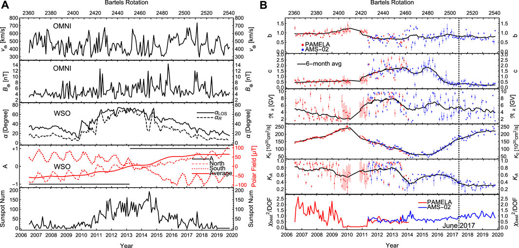
Figure 1. The time series of the four observational parameters (A), and the five fitted parameters through the MCMC process and the corresponding ${\chi }^2$ (B). In the left panels, all the observables have been smoothed by their averages over each Bartels rotation (27 days) for better visual, but in real calculations higher time resolution data are used. The WSO provide two versions of the HCS tilt angle definitions, here we use the classical “line-of-sight” definition (solid curve), but also plot the “radial” definition (dashed curve) for reference. The polarity $A$ is defined as the sign of the averaged solar polar magnetic field, and this average is defined through the north and south polar magnetic field, here they are plotted altogether. The sunspot number (SSN) is another frequently used observable for solar activity, so we have also plotted for reference. In the right panels, for each variable we also plot the smoothing of 6 months’ average. Fitting prior to June 2017 has already been given by Song et al. (2021).

2.1.1 Solar wind

The solar wind velocity up to the termination shock is given by Potgieter et al. (2014)

${\vec{v}}_{\text{sw}}\left(r,\theta \right)=v_{\oplus }\left(1-\exp \left[\frac{40}{3}\left(\frac{r_{\odot }-r}{r_{\oplus }}\right)\right]\right)\left(1.475-0.4\tanh \left[6.8\left(\alpha +\frac{\pi }{12}-\left|\theta -\frac{\pi }{2}\right|\right)\right]\right){\vec{e}}_r,(4)$

where $v_{\oplus }$ is the observed solar wind speed near Earth, for which we use the daily OMNI data. $r_{\odot }=0.005$ AU is the radius of the Sun, $r_{\oplus }=1$ AU is the radial position of the Earth. $\alpha$ is the observational tilt angle of the wavy heliospheric current sheet (HCS) from the L model, and we use the Wilcox Solar Observatory data which is given every 10 days. The first bracketed factor describes the radial acceleration behavior of the solar wind. After the acceleration, the speed remains almost constant until reaching the termination shock. The second bracketed factor describes the behavior in the polar direction. At two polar directions ($\theta \to 0$ and $\theta \to \pi$) and/or for a small tilt of the HCS $\alpha$ (or during weak solar activity), the factor tends to be large and approaches 1.875. And for locations near the equator and/or for a large $\alpha$ (or during strong solar activity), the factor tends to be small and approach 1.075 (Potgieter et al., 2014). This depiction of the spatial and temporal distribution of the solar wind is valid up to the termination shock.

Outside the termination shock of 90 AU, the solar wind transitions from supersonic to subsonic speeds. Here, the velocity is assumed to decrease to $40\%$ of the value just inside the termination shock (Li et al., 2008), then follow an inverse square law $(r^{-2})$ as further moves out. The heliosheath is acting as a “modulation barrier”, in which our solar wind does not expand, exerting no adiabatic cooling effect on the incoming GCR particles. The enhanced modulation observed in the heliosheath is not accounted for in our calculation, and our modeling is not entirely accurate or comprehensive. However, we expect that this inconsistency will not have a significant numerical impact on our final spectra calculation, as our focus of the inner solar system region of $1.0-1.6$ AU is very far from the heliosheath. Moreover, there is some dependence of the inferred local interstellar spectra on the modulation process in the heliosheath, consequently the calculated GCR spectra (Langner and Potgieter, 2004; Langner et al., 2003).

2.1.2 Heliospheric magnetic field

The used 3D HMF is the Parker’s spiral with a polar region enhancement (Jokipii and Kota, 1989).

$\vec{B}\left(r,\theta ,\varphi \right)=-\frac{A{B}_{\oplus }}{r^2}\mathrm{s}\mathrm{g}\mathrm{n}\left[\theta -{\theta }^{\prime }\right]\left({\vec{e}}_{\text{r}}+\xi {\vec{e}}_{\theta }-\mathrm{\Psi }{\vec{e}}_{\mathrm{\phi }}\right),(5)$

${\theta }^{\prime }=\frac{\pi }{2}-{\tan }^{-1}\left[\tan \alpha \sin \left[\varphi +\frac{\left(r-r_{\odot }\right)\mathrm{\Omega }}{v_{\text{sw}}}\right]\right],(6)$

$\xi =\frac{r{\delta }_m}{r_{\odot }\sin \theta },(7)$

$\mathrm{\Psi }=\frac{\left(r-r_{\odot }\right)\mathrm{\Omega }\sin \theta }{v_{\text{sw}}}.(8)$

Here, $A=\pm 1$ is the observed polarization of the HMF, being positive (negative) indicates that the HMF points outward (inward) in the northern hemisphere of the Sun. $B_{\oplus }$ is the observational HMF strength near the Earth. The sources of the $A$ and $B_{\oplus }$ are also the above Wilcox Solar Observatory data and the daily OMNI satellite data, respectively. The $\mathrm{s}\mathrm{g}\mathrm{n}(x)=x/|x|$ is the signum function. $\mathrm{\Omega }=2.66\times 10^{-6}/$s is the angular rotation speed of the Sun. The colatitude ${\theta }^{\prime }$ is the separation between the north and south hemispheres caused by the undulating HCS at the phase angle $\varphi$. In addition to the standard Parker spiral, the term $\xi {\vec{e}}_{\theta }$ acts as a correction for the observed HMF increase at a large radial distance in the polar heliosphere. This term ensures divergence-free behavior, as introduced by Jokipii and Kota (1989). Here, the perturbation parameter in the equatorial plane ${\delta }_m$ is set to be $2\times 10^{-5}$ (Qin and Shen, 2017; Boschini et al., 2016). To avoid a singularity, ${\delta }_m/\sin \theta$ is set equal to the value ${\delta }_m/\sin (1°)$ when $\theta <1°$ or $\theta >179°$ (Raath et al., 2016).

2.1.3 Diffusion and drift coefficients

In contrast to the two aforementioned models which are determined through observation and have become quite distinctive, there are numerous options in the literature for diffusion and drift coefficients. Here, we use a set of parameterized coefficients as provided by Potgieter (2013). Compared with diffusion coefficients that are more theoretically motivated (e.g., Qin and Zhang, 2014), our parametrized coefficients usually have the advantage of reproducing observational spectra with greater precision, but at the cost of complexity in making forecast.

The drift velocity is given by Potgieter (2013)

$\begin{array}{ll}\hfill {\vec{v}}_{\text{d}}& \left(\mathfrak{R},r,\theta ,\varphi \right)=\nabla \times \left(K_A\frac{\mathrm{s}\mathrm{g}\mathrm{n}\left[q\right]\mathfrak{R}\beta }{3}\frac{{\left(\mathfrak{R}/{\mathfrak{R}}_A\right)}^2}{1+{\left(\mathfrak{R}/{\mathfrak{R}}_A\right)}^2}\frac{\vec{B}}{B^2}\right),\hfill \\ \hfill & =-K_A\frac{\mathrm{s}\mathrm{g}\mathrm{n}\left[q\right]\mathfrak{R}\beta }{3}\frac{{\left(\mathfrak{R}/{\mathfrak{R}}_A\right)}^2}{1+{\left(\mathfrak{R}/{\mathfrak{R}}_A\right)}^2}\frac{A}{B_{\oplus }}\left(\mathrm{s}\mathrm{g}\mathrm{n}\left[\theta -{\theta }^{\prime }\right]\nabla \times \vec{g}\right.\hfill \\ \hfill & \left.- \delta \left(\theta -{\theta }^{\prime }\right)\vec{g}\times \nabla \left(\theta -{\theta }^{\prime }\right)\right),\hfill \end{array}(9)$

with

$\vec{g}=\frac{r^2\left({\vec{e}}_r+\xi {\vec{e}}_{\theta }-\mathrm{\Psi }{\vec{e}}_{\phi }\right)}{1+{\xi }^2+{\mathrm{\Psi }}^2}.(10)$

Here, $\mathfrak{R}=pc/q$ is the rigidity of the particle, and for nonrelativistic case the particle momentum $p=mv$. $m$ and $v$ are the mass and speed of the particle, respectively, and $q$ is the particle’s charge. $K_A$ is the overall dimensionless drift coefficient to be fitted, which ranges from 0 to 1, with $K_A=1$ describing undisturbed drift without the competition of scattering. $\beta =v/c$ is the ratio of the particle’s speed to the speed of light. Note that this ratio is an implicit function of rigidity, as $\beta =pc/E=Ze\mathfrak{R}/\sqrt{{(Ze\mathfrak{R})}^2+m^2{c}^4}$. ${\mathfrak{R}}_A=0.9$ GV empirically, and the corresponding factor smoothly connects the high rigidity drift region and the low rigidity scattering region, where small-scale turbulence plays a central role. $B$ is the magnitude of the HMF.

The diffusion tensor is given by its components (Potgieter, 2013).

$K_{\Vert }=K_0\beta \left(\frac{\sqrt{1+{\mathrm{\Psi }}^2}{B}_{\oplus }}{B}\right){\left(\frac{\mathfrak{R}}{{\mathfrak{R}}_0}\right)}^b{\left(\frac{{\left(\mathfrak{R}/{\mathfrak{R}}_0\right)}^3+{\left({\mathfrak{R}}_K/{\mathfrak{R}}_0\right)}^3}{1+{\left({\mathfrak{R}}_K/{\mathfrak{R}}_0\right)}^3}\right)}^{\frac{c-b}{3}},(11)$

$K_{\perp ,r}=0.02K_{\Vert },(12)$

$K_{\perp ,\theta }=\left(2+\tanh \left[8\left(\left|\theta -\frac{\pi }{2}\right|-\frac{7\pi }{36}\right)\right]\right)K_{\perp ,r}.(13)$

Here $K_0$ is the overall diffusion coefficient to be fitted in units of $10^{20}{\mathrm{c}\mathrm{m}}^2/\mathrm{s}$, ${\mathfrak{R}}_0=1$ GV empirically. The coefficient is a smooth connection of two asymptotic power laws, with their indices of $b$ and $c$ to be fitted for the low and high rigidity region, respectively. The last parameter to be fitted is ${\mathfrak{R}}_K$, which determines the transition to the asymptotic power law on the high rigidity side.

Finally we would like to make comment on the validity of the spectra calculation at locations different from the 1.0 AU. Since all of the above models hold for the entire spatial heliosphere region, for given observational and fitted parameter in time series, the calculation of GCR spectra is equally accurate at other locations within the heliosphere, especially at the range of $1.0-1.6$ AU between the orbits of Earth and Mars. In fact, the current work is extending the scope of our previous work by generalizing the 1.0 AU slice provided in Song et al. (2021); Chen et al. (2023) to other radial locations. The same generalization is conceptually claimed by other similar SDE works as well (e.g., Boschini et al., 2022).

2.2 The data source and fitting

As mentioned, the Alpha Magnetic Spectrometer (AMS) 02 detector is one of the most effective tools for measuring GCR spectra. It was launched in May 2011 and installed on the International Space Station at an altitude of about 400 km. The detector can measure all the GCR elements with atomic numbers ranging from 1 to 28, with a strong capability for discriminating between elements and controlling errors. The PAMELA detector is another space-borne magnetic spectrometer before the AMS-02, which was launched in June 2006 into an orbit at an altitude of $350-600$ km. As magnetic spectrometers, both of them utilize the Lorentz force to bend the trajectory of incident charged particles. By measuring the deflection as well as the energy loss in the detector, the charge of GCRs can be precisely determined (Aguilar et al., 2021), which is crucial for dosimetry. On the other hand, the two spectrometers are still in the geomagnetic field, which will partially shield the incident GCR from being measured, particularly for low rigidities. But such shielding effect depends on geographic location and direction. By selecting the events above the geographic-location-and-direction dependent geomagnetic cutoff rigidity determined in the backtracing process (e.g., see Aguilar et al., 2015), the AMS and PAMELA group were able to discriminate and measure the primary GCR down to low rigidities in high latitude region. Both spectrometers have published time-dependent spectral measurements for the GCR proton and helium (the solar energetic particle flux has been manually removed already in the published data), which consist of approximately $88\%$ and $11\%$ of GCR flux respectively. Measurements for heavier elements as well as extended time span are underway at the AMS-02.

We determine the time-series of the aforementioned five parameters by fitting them to the time-dependent spectra measured by AMS-02 and PAMELA in the proton and helium channels (Adriani et al., 2013; Martucci et al., 2018; Marcelli et al., 2020; Aguilar et al., 2018; 2021; 2022). In Figure 1 we have plotted the four observables ($v_{\oplus }$, $B_{\oplus }$, $\alpha$, and $A$) in the left panel and the five fitted parameters ($b,c,{\mathfrak{R}}_K,K_0$, and $K_A$) in the right panel as time series. For each Bartels rotation, or every 27 days, fitting is performed using a Markov Chain Monte Carlo method (Song et al., 2021; Chen et al., 2023). In the relevant SDE simulation, it takes some time for each pseudoparticle to move backward and reach the heliopause. During this time, we use the time-dependent solar wind and HMF. Specifically, we implement a stepwise approach using the observed time series of $v_{\oplus },B_{\oplus },\alpha ,A$, while assuming that the fitting parameters $b,c,R_k,K_0,K_A$ remain constant. The 6-month average of the fitted time series in Figure 1 is only used to provide a clear depiction of the trend for each quantity, and we utilize the best fit at each time point. There is an overlap period for the PAMELA and AMS-02 experiments, but in the plot, they are treated as independent fits.

The GCR spectra data are provided in the form of time series only for the proton and helium channels. Therefore, the fitting of diffusion and drift coefficients is performed only for these two species. However, Song et al. (2021) was able to fit both the proton channel and the helium channel with the same parameter set. This indicates the universality of the diffusion and drift coefficients for different GCR species (Tomassetti et al., 2018; Corti et al., 2019; Wang et al., 2019; Ngobeni et al., 2020; Fiandrini et al., 2021). In fact, the diffusion and drift coefficients are statistical measures of the small and large scale magnetic field irregularities. For GCRs with the same rigidity, the local curvature radius of the trajectory of an incident charged particle is determined by the ratio of the rigidity to the magnetic field strength, regardless of the particle’s type or mass. It implies the same trajectory for particles with the same rigidity, explaining the universality of the drift coefficient for all GCR species. On the other hand, the diffusion coefficient is determined by the interaction between particles and waves/turbulence. According to quasi linear theory, the particle with the same gyro-radius resonates with the same waves, thus the resonant condition determines that particles with the same rigidity have the same diffusion coefficient. So here we use the best fits of the combined proton and helium data as the universal coefficients, and apply them to calculate the other 26 elements.

3 The calculated GCR spectra

The GCR flux is calculated on a four-dimensional grid, which is summarized in Table 1. Figure 2 shows sample calculations for three dimensions at 1.0 AU, namely during solar minimum and maximum as two representative dates, in each panel for five representative GCR species and the whole rigidity range.

Table 1

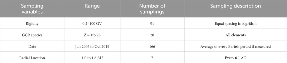
Table 1. The list of variables for our current SDEMMA spectra. The major part of the calculation consists of $91\times 28\times 166\times 7=2960776$ data points. The flux for each point is based on a statistics of 3,000 pseudoparticles.

Figure 2

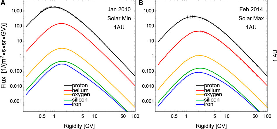
Figure 2. The SDE calculated spectra for proton (black), helium (red), oxygen (orange), silicon (green), and iron (blue) at 1.0 AU, at the solar minimum (A) and maximum (B) respectively. The PAMELA and AMS-02 measured proton and helium GCR spectra for the corresponding periods are also shown, except for the PAMELA helium data which is not for one Bartels rotation. Due to the finite sampling number in the SDE method (3,000 pseudoparticles per energy bin), the spectra show some fluctuation on the low rigidity side (see also discussion in Section 3.4).

3.1 The rigidity

The calculated range of rigidity is always from 0.2 to 100 GV for all elements. As a result of the MCMC fitting process, the calculated spectra accurately reproduce the measured proton and helium spectra in the rigidity region where PAMELA and AMS-02 have conducted direct measurements (Song et al., 2021; Chen et al., 2023), as a validation of the model. However, due to the finite thickness of the apparatus, low-energy/rigidity GCRs are blocked in the detector and cannot be detected, causing the measured rigidity to terminate at 1 GV for a proton and 1.65 GV for helium for the AMS-02. Beneath these minimal rigidities, one must work with the calculated spectra. As seen in Figure 2, the flux asymptotically vanishes as the rigidity decreases on the low-rigidity side (Moraal and Potgieter, 1982). The GCR spectra also decrease on the high rigidity side, following a power law with a well-known spectral index of approximately $-2.7$.

3.2 The GCR species

Although heavy ions are less abundant, their dose contribution can be enhanced by powers of their nuclear charge $(Z)$, due to the nature of the Bethe-Bloch stopping power as well as the biological effectiveness. As a result, their dose contribution can be comparable to that of protons or helium. In the 1.0 AU calculation of Chen et al. (2023), it is noted that the five elements shown in Figure 2 together with magnesium are the most significant contributors to radiation dose, accounting for over $70\%$ of the unshielded astronaut effective dose equivalent. These elements also represent all fractional contributions greater than $5\%$ from a single element. Due to the smallness of the radial gradient, as demonstrated below, we expect that this behavior will persist across the entire spatial range.

The AMS-02 measurements for heavy elements extend to silicon and iron channels, but they are now in the form of averages over many years, and results with even shorter period have not been published yet. On the other hand, the ACE/CRIS experiment provides time-dependent measurement for heavy elements, but the detector type is calorimeter rather than magnetic spectrometer. Since we define our model using only the time-dependent data from space-borne magnetic spectrometers, the ACE/CRIS data for heavy elements are used only for cross check, but not for fitting. We respect the aforementioned universality of the diffusion and drift coefficients in calculations of other heavy elements for theoretical consistency. In Chen et al. (2023) we have compared our calculated spectra to the measurements averaged over many years for the elements with available data, and found good agreement.

3.3 The time dependence

Solar activity is known for its stochastic fluctuations in addition to its well-known 11-year cycle, which consists of a solar maximum and a solar minimum in each cycle. Many issues related to the time dependence have already been addressed in the previous discussion of Section 2.2. One can also refer to Song et al. (2021) for more information about the GCR spectra prior to June 2017, and a comparison in the form of dose rate time series in Chen et al. (2023) for the 1.0 AU slice result.

Starting from June 2006 of the beginning of the PAMELA experiment (Adriani et al., 2013; Martucci et al., 2018; Marcelli et al., 2020), the original fitting up to June 2017 in Song et al. (2021) is further extended to October 2019, in order to match the latest available AMS-02 time-dependent proton and helium data (Aguilar et al., 2018; Aguilar et al., 2021; Aguilar et al., 2022). New data after October 2019 will be implemented as soon as they become available.

Currently the model does not include forecast for future GCR spectra, which is crucial for future spacecraft design and space mission planing. For future solar modulation, all the GCR spectra forecast should be based on the forecast of future heliospheric environment parameters. A new GCR spectra forecast approach has been developed with the machine learning technique in Du et al. (2025), which uses the same previous GCR spectra data but not the Parker’s transport equation. A more traditional approach of forecast based on solving the Parker’s transport equation, more similar to the current forecast of Badhwar-O’Neil model and HelMod model, is also under development.

3.4 The radial dependence

In Gieseler et al. (2008) the radial gradient was measured to be $(4.5\pm 0.6)\%$/AU in the $125-200$ MeV/n helium channel and the $147-198$ MeV/n carbon channel during 1997–2006. The two above channels both correspond to a bin of central rigidity of 1.122 GV in our calculated spectra. The fact that higher GCR flux is observed at an outer position can be simply explained by the scattering of the GCR particles in the heliosphere, that part of the GCRs can be scattered back into the interstellar medium as they enter the heliosphere. As they enter deeper, more GCRs will be scattered back, and the flux will be lower.

In Figure 3 we present several flux ratios $J(r)/J(1.0\text{AU})$ as functions of the radial position. We can observe a distinct positive radial gradient, at least for the two solar maximum configurations. The radial gradient for the astronaut’s radiation dose should be closer to the radial gradient of the total integrated flux, rather than that of the representative low rigidity bin of 1.122 GV. In our calculation, we can clearly distinguish the radial dependence between a solar minimum and a solar maximum, with that at a solar maximum noticeably larger. The measurement made by Gieseler et al. (2008) over a period of 9 years can be considered as a weighted average, yeilding a radial gradient between our solar minimum case and the maximum case of the corresponding 1.122 GV bin.

Figure 3

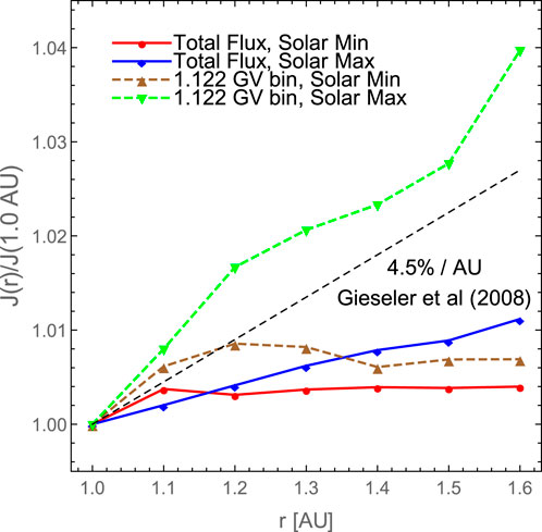
Figure 3. The flux $J(r)/J(1.0\text{AU})$ ratios as a function of radial position $r$ between 1.0 and 1.6 AU. For both the “total flux” integrated over the $0.2-100$ GV rigidity range and the single bin flux, their values at various locations are normalized with the respective values at Earth ($r=1.0$ AU), then further averaged over all the $Z=1-28$ elements in order to reduce statistical fluctuations. The single bin $J(r)$ of 1.122 GV best matches the previous measurement of Gieseler et al. (2008) of the helium $125-200$ MeV/n ($0.997-1.285$ GV) bin and the carbon $147-198$ MeV/n ($1.088-1.278$ GV) bin. The gray dashed line shows the measured central value of $4.5\%/$AU of Gieseler et al. (2008).

In Figure 4 we plot the flux ratios $J(r)/J(1.0\text{AU})$ as a function of rigidity for two extreme epochs. The previous Figure 3 has already shown that the radial gradient is greater at low rigidities and smaller at high rigidities. Such phenomena are being continuously demonstrated now. Here we do not directly use the calculation results described in Table 1 with the default statistics of 3,000 pseudoparticles each, but increase the statistics to $10^6$ each to reduce the statistical noise. In summary, as we have demonstrated, the radial gradient consistently remains small for any GCR element at any given time. Ignoring this gradient may result in a maximum error of only a few percents.

Figure 4

Figure 4. The proton flux $J(r)/J(1.0\text{AU})$ ratios as a function of rigidity, for six radial positions and two solar modulation conditions: solar minimum [January 2010, (A)], and solar maximum [February 2014, (B)]. The errorbar is from a simple $1/\sqrt{N}$ estimation with $N=10^6$ (dedicated running with high statistics).

Note that there are various techniques for solving Parker’s transport equation. Beyond the SDE method, there is another class of method, which is the alternating directional implicit (ADI) method (Potgieter and Moraal, 1985). Different from the SDE method which introduces the stochastic motion for a traced pseudoparticle and solves the problem in a Monte Carlo way, the ADI method focus on directly solving the partial differential equation in a deterministic way. In the latter approach a static equilibrium phase space density flow configuration is solved, then information across the whole spatial region is immediately extracted. On the other hand, in the SDE method the calculation of spectrum can only be done spatial point by spatial point, so if a radial gradient is the primary goal the SDE calculation is relatively less effective. But since the sampled pseudoparticle is simulated in real time, as mentioned before we can adopt a dynamical heliospheric environment with the observed $v_{\oplus },B_{\oplus },\alpha ,A$ time series. This is an advantage over the ADI method, the assumed static heliospheric environment of which is indeed inconsistent with its nature of time variability.

3.5 Comparison with other models

In Table 2 we present a simple comparison of our SDEMMA model with other recent GCR models, including the latest version of the Badhwar-O’Neill models (O’Neill et al., 2015; Slaba and Whitman, 2019) and the HelMod model (Boschini et al., 2016). All versions of NASA’s Badhwar-O’Neill models are based on a one-dimensional (radial) solution to Parker’s transport equation. Only one time-dependent variable, the modulation potential ${\varphi }_Z$, is developed to control the modulation effect, but for different element it is fitted to different values. In the latest 2020 version, the data set used for fitting is the ACE/CRIS data, when available, and the SSN is used otherwise. On the other hand, similar to ours, the HelMod model is also based on the SDE solution of Parker’s full (two-dimensional) transport equation. The SSN and CR neutron monitor data are used to fit the modulation. For both the Badhwar-O’Neil 2020 model and the HelMod model, the AMS-02 and PAMELA time-dependent spectra are used for calibration at a level of average over many years, but not for exact direct fitting of the solar modulation time series. It is natural that our GCR model provides better agreement with the AMS-02 and PAMELA data as the baseline, with an average absolute relative difference $|Rd|$ (O’Neill et al., 2015) of less than one percent in the proton and helium channels. In comparison, the Badhwar-O’Neill 2020 model and the HelMod model show an average absolute relative difference of about $3\%$.

Table 2

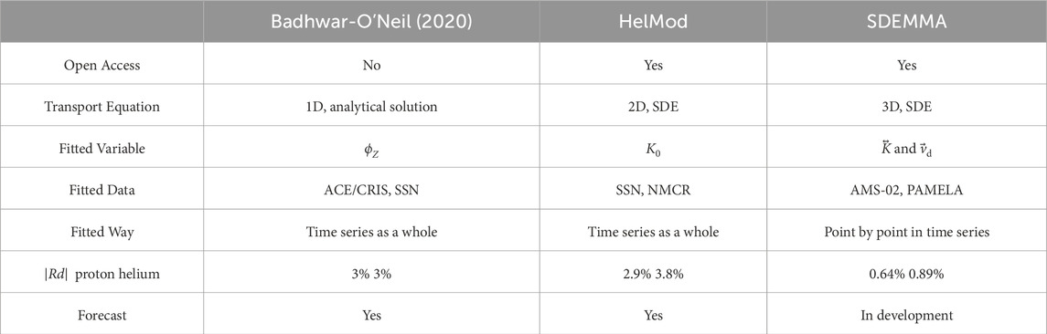
Table 2. Comparison of the Badhwar-O’Neil 2020 model, the HelMod model and our SDEMMA model.

A dedicated and more comprehensive comparison of GCR models is given in Liu et al. (2024), which includes our model, the BON2020 model, the HelMod model, as well as the CREME model (Tylka et al., 1997; Adams et al., 2012) and DLR model (Matthiä et al., 2013).

4 Induced dose equivalent rate between Earth’s and Mars’ orbit

Based on the SDEMMA model, we calculate the astronaut dose equivalent rate $\dot{H}$ induced by the isotropic GCR flux between the Earth’s and the Mars’ orbit. It is given by

$\dot{H}={\displaystyle \sum _{\text{R}}}\int d\mathfrak{R}4\pi \frac{d^4{N}_{\text{R}}}{dAdtd\mathrm{\Omega }d\mathfrak{R}}\frac{\left(\mathrm{\Delta }{E}_{\text{R}}/m\right)Q}{d{N}_{\text{R}}/dA}={\displaystyle \sum _{\text{R}}}\int d\mathfrak{R}4\pi J_{\text{R}}\left(\frac{D_{\text{R}}Q}{{\mathrm{\Phi }}_{\text{R}}}\right).(14)$

By cancelling the factors such as $d\mathfrak{R}$, $d{N}_{\text{R}}$ and $dA$, the first equation reduces eventually to $\dot{H}\sim (\mathrm{\Delta }{E}_{\text{R}}/m)Q/t$ as the definition of dose equivalent rate with all particles’ contribution. And in the second equation, the two factors reduce respectively to the GCR spectra $J_{\text{R}}(\mathfrak{R})=\frac{d^4{N}_{\text{R}}}{dAdtd\mathrm{\Omega }d\mathfrak{R}}$ and the fluence-to-dose-equivalent conversion coefficients $\frac{D_{\text{R}}Q}{{\mathrm{\Phi }}_{\text{R}}}=\frac{(\mathrm{\Delta }{E}_{\text{R}}/m)Q}{d{N}_{\text{R}}/dA}$. Here $N_{\text{R}}$ is number of incident particle of radiation “R”, $A$ is a cross section of the incident particle beam, $\mathrm{\Omega }$ is the solid angle for the incident flux. $\mathrm{\Delta }{E}_{\text{R}}$ is the energy loss of radiation “R”, $m$ is the corresponding target mass, so $D_{\text{R}}=\mathrm{\Delta }{E}_{\text{R}}/m$ is the energy deposited in unit mass, namely the absorbed dose. $Q$ is the quality factor which converts the physical absorbed dose to the medical dose equivalent, which has two definitions: the ICRP60 definition (ICRP60, 1991) and the NASA definition (Cucinotta et al., 2011). ${\mathrm{\Phi }}_{\text{R}}=d{N}_{\text{R}}/dA$ is the fluence for radiation “R”.

The fluence-to-dose-equivalent conversion coefficient has the meaning of the expected dose equivalent caused by a single incident particle, if the incident particle is integrated over all contributing area on the normal plane of its “beam” direction. It is calculated by particle physics Monte Carlo code. We have calculated the isotropic fluence-to-dose-equivalent conversion coefficients using the Monte Carlo toolkit GEANT4 (Agostinelli et al., 2003; Allison et al., 2006; Allison et al., 2016) using the ICRU sphere¹ as the dose counter, for all the $Z=1-28$ GCR elements and $27-36$ energy points ranging from 1 MeV/n to 100 GeV/n for each element. Except for using the simplified target of the ICRU sphere rather than the detailed human voxel phantom (ICRP110, 2009), the calculation procedures are the same as the series of independently developed dose coefficient sets by ourselves (Chen et al., 2025), such as the linear energy transfer and quality factor calculation methods. Compared with the only published dose coefficient set of ICRP123 (2013) for the same $Z=1-28$ elements and energy range and the detailed human voxel phantom, we have the freedom to considered characteristic shielding configurations as an essential improvement of the naked human phantom assumption. This is achieved by setting an extra shielding shell around the target dose counter in the world construction of the simulation, where the shell has a certain dimension, shape, and chemical composition. Then the simulated incident particle will interact with the shielding structure before it hits the dose counter. The shielded dose coefficients are defined as the expected (average) dose equivalent caused by a single incident particle before entering any shielding.

4.1 Unshielded case

The first $\dot{H}$ calculation set is for the unshielded case, and the results using the ICRP60 quality factor are collected in Figure 5. We have tested several combinations of different GCR spectra models (our SDEMMA model and the alternative HelMod model (Boschini et al., 2016)) with different fluence-to-dose-equivalent conversion coefficients (the ICRP123 dose coefficient (ICRP123, 2013), our independently calculated dose coefficient set using the ICRP110 human voxel phantom (Chen et al., 2025), and our independently calculated dose coefficient set using the ICRU sphere). Since the SDEMMA model provides GCR spectra at seven different radial locations at per 0.1 AU, the range of the seven $\dot{H}$ values form a small vertical bar for each time point. Moreover, based on the ICRP110 human voxel phantom, the first three calculations yield dose equivalent rates ${\dot{H}}_{\text{T}}$ for each of the 15 sensitive organs/tisse “T”, and the $\dot{H}$ shown is the weighted sum of the ${\dot{H}}_{\text{T}}$s by the tissue weight factor (ICRP103, 2007) (the effective dose equivalent). We can see that the dose equivalent rate differences between the HelMod and the SDEMMA GCR models are smaller than those between different dose coefficient sets of $\sim 11\%$. $\dot{H}$ for detailed human voxel phantom are $3\%-5\%$ lower than those for the ICRU sphere.

Figure 5

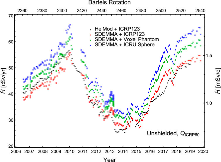
Figure 5. The unshielded dose equivalent rate $\dot{H}$ time series during June 2006 and October 2019, for four combinations of GCR models and fluence-to-dose conversion coefficients: the HelMod model combined with the ICRP123 dose coefficient (black points), the SDEMMA model combined with the ICRP123 dose coefficient (red vertical bars), the SDEMMA model combined with our independently calculated dose coefficient set using the ICRP110 human voxel phantom (green vertical bars), and the SDEMMA model combined with dose coefficient calculated use the ICRU sphere (blue vertical bars). For SDEMMA models, vertical bars indicate the range of $\dot{H}$ achieved in the radial range of $1.0-1.6$ AU. And for the first three combinations which are all based on detailed human phantoms, $\dot{H}$ shown is the weighted (by the tissue weighting factor) sum of the dose equivalent rates of 15 sensitive organs/tissues.

4.2 MSL/RAD shielding

The MSL/RAD shielding during the cruise stage in the transit orbit is too complicated to simulate exactly. In simulation we simplify the shielding to three aluminum layers: $30\%$ of the detector acceptance is shielded by a mass thickness of 1 g/cm², $50\%$ is shielded by a mass thickness of 9 g/cm², and the remainder $20\%$ is shielded by a mass thickness of 56 g/cm². The average is 16 g/cm², the same as the averaged MSL/RAD shielding thickness. On the other hand, beneath the shielding the mass thickness of the detector is small, giving negligible self-shielding. Therefore, the target dose counter has been manually divided into the surface part (with 2 mm thickness) and the remainder part. The surface part emulates the detector with negligible self-shielding, and the remainder should give values closer to the effective dose equivalent of real human phantom.

We have performed two round of simple simulations. The first one also using the same isotropic GCR incidence and the ICRU sphere gives a dose equivalent rate of 2.07 mSv/d averaged over the MSL/RAD time window. While the isotropy is the case for the astronaut in deep space, the MSL/RAD detector has a small field of view of $30°$ (Zeitlin et al., 2013). While an energetic particle can penetrate the dose counter and induce dose on the other side opposite to its incidence, this cannot be measured by the MSL/RAD. The second simulation uses a plane beam and target, and gives a dose equivalent rate of 1.20 mSv/d if the flux is scaled to $4\pi$ solid angle. The MSL/RAD measured dose equivalent rate of $1.75\pm 0.30$ mSv/d purely from the GCR contribution (Guo et al., 2015) is between the two. Note that the remainder part of the dose counter in the two simulations both give smaller dose-equivalent rates $(\sim 50\%-\sim 70\%)$, due to the self-shielding.

4.3 Optimized 30 g/cm² shielding

The last $\dot{H}$ calculation set is for shieldings with mass thickness of 30 g/cm². In addition to the Bethe-Bloch stopping effect which slows down the incident particle and decreases the dose, shielding materials also produce secondary particles when hit by energetic incident particle, and those secondary particles can contribute dose when hitting the astronaut as well. For light proton and helium the secondary particles will eventually increase the dose. So there is an optimized depth which balances the production of secondary particles (increase with shielding depth) and the Bethe-Bloch stopping, and the depth is determined to be 30 g/cm² (Guo et al., 2017).

Figure 6 shows our final $\dot{H}$ calculation with the ICRU sphere and optimized shielding mass thickness. As for shielding material, aluminum is currently widely used in space as structural material, but polyethylene is an optimized baseline choice for its high electron-number-to-mass ratio which facilitates the Bethe-Bloch stopping effect (Naito et al., 2020). We have also varied the quality factor $Q$ definition. As seen, at the flux minimum in the covered period, the dose equivalent rates induced by GCR behind optimized polyethylene shielding are $\sim 14$ cSv/yr using the ICRP60 quality factor and $\sim 17$ cSv/yr using the NASA quality factor, while at the flux maximum the rates are $\sim 25$ cSv/yr and $\sim 30$ cSv/yr, respectively.

Figure 6

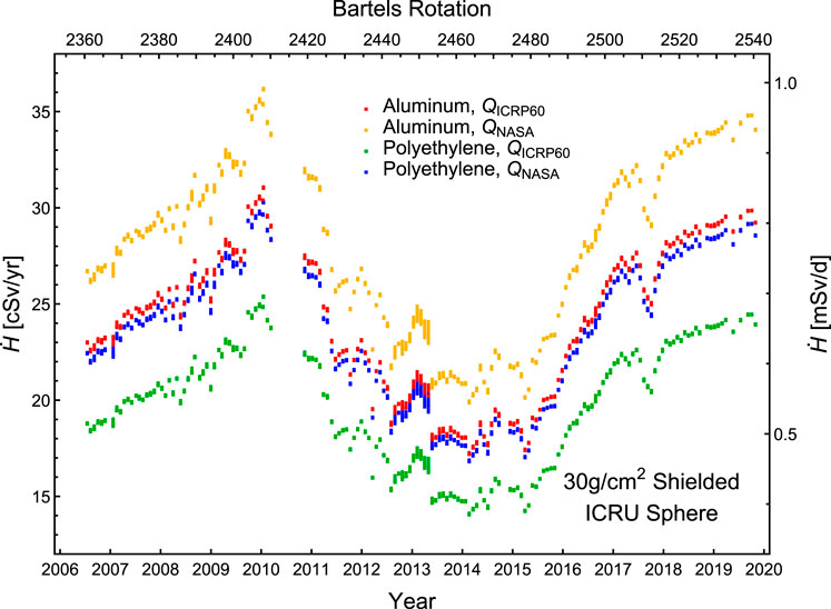
Figure 6. The dose equivalent rate $\dot{H}$ time series during June 2006 and October 2019 for the ICRU sphere, after an optimized shielding with depth of 30 g/cm². Here we have considered the two materials of aluminum and polyethylene for the shielding structure, and two quality factors of $Q_{\text{ICRP}60}$ and $Q_{\text{NASA}}$ in the dose equivalent calculation.

The fluence-to-dose-equivalent conversion coefficient and dose equivalent rate calculation using the detailed human voxel phantom will be provided in a forthcoming publication.

5 Summary

We have presented a model for the modulated galactic cosmic ray spectra called SDEMMA. This model is based on data from the space-borne magnetic spectrometers PAMELA and AMS-02. In this model, we use the 3D stochastic differential equation method (Equations 2, 3) to calculate spectra, incorporating the recently developed local interstellar spectra of galactic cosmic rays for all the $Z=1-28$ elements. Heliospheric environment modelings based on observational inputs and MCMC fittings are used. This model enables us to precisely reproduce the time-dependent measurements of PAMELA and AMS-02 (Adriani et al., 2013; Martucci et al., 2018; Marcelli et al., 2020; Aguilar et al., 2018; 2021; 2022) with a margin of error of just a few percent, regardless of energy and GCR species. We extend the spectra calculation to other radial locations in the inner solar system beyond the previous focus at 1.0 AU, which is relevant to the Mars mission.

We have also developed a set of fluence-to-dose-equivalent conversion coefficients based on simplified dose counter but several shielding considerations. Combining the SDEMMA GCR model and the dose coefficients, the astronaut radiation dose equivalent rates on the transfer orbit are calculated using Equation 14, for the considered period with an explicit radial dependence.

Data availability statement

The SDEMMA dataset for GCR spectra time series can be downloaded as a zip file from https://en.iat.cn/resource.

The OMNI solar wind and HMF data are available from the GSFC website https://omniweb.gsfc.nasa.gov. The Wilcox Solar Observatory HCS data is available from the WSO website http://wso.stanford.edu/. The sun spot number data is available from the Solar Influences Data analysis Center website https://www.sidc.be.

The PAMELA proton and helium spectra time series can be extracted from https://tools.ssdc.asi.it/CosmicRays/chargedCosmicRays.jsp. The AMS-02 proton and helium spectra tables in time series are available via the corresponding supplemental material and data links of Phys. Rev. Lett. 121, 051101 (2018), Phys. Rep. 894, 1 (2021), and Phys. Rev. Lett. 128, 231102 (2022) at the AMS group publication page https://ams02.space/publications.

The HelMod GCR spectra time series are available from https://www.helmod.org/index. php?view=article&id=76:transfer-orbit-fluence&catid=14. The fluence-to-dose-equivalent conversion coefficients for the ICRU sphere can be downloaded as a zip file from https://en.iat.cn/resource.

The ICRP123 fluence-to-dose-equivalent conversion coefficients are available via the “Supplemental Material” link at the ICRP123 publication URL https://www.icrp.org/publication.asp?id=ICRP%20Publication%20123.

Author contributions

XS: Data curation, Formal Analysis, Investigation, Methodology, Resources, Software, Validation, Writing–review and editing. RH: Conceptualization, Funding acquisition, Project administration, Supervision, Visualization, Writing–original draft, Writing–review and editing. SX: Data curation, Writing–review and editing. XC: Data curation, Writing–review and editing. XL: Funding acquisition, Methodology, Software, Writing–review and editing.

Funding

The author(s) declare that financial support was received for the research and/or publication of this article. The presented work was supported by the Shandong Institute of Advanced Technology start funding (2020106R01, 2020106R02) and the NSFC grants (U2106201).

Acknowledgments

We are grateful to the useful discussion with Jingnan Guo, Tong Su, Weiwei Xu and Vladimir Mikhailov. The generative AI of Wordvice AI and DeepSeek-R1 have been used for English improvement.

Conflict of interest

The authors declare that the research was conducted in the absence of any commercial or financial relationships that could be construed as a potential conflict of interest.

Publisher’s note

All claims expressed in this article are solely those of the authors and do not necessarily represent those of their affiliated organizations, or those of the publisher, the editors and the reviewers. Any product that may be evaluated in this article, or claim that may be made by its manufacturer, is not guaranteed or endorsed by the publisher.

Footnotes

¹The ICRU sphere is a phantom used in radiation protection. It has a diameter of 30 cm, and a hypothetical tissue equivalent material of density 1 g/cm3 and composition of oxygen $76.2\%$, carbon $11.1\%$, hydrogen $10.1\%$ and nitrogen $2.6\%$.

References

Adams, J. H., Barghouty, A. F., Mendenhall, M. H., Reed, R. A., Sierawski, B. D., Warren, K. M., et al. (2012). Creme: the 2011 revision of the cosmic ray effects on micro-electronics code. IEEE Trans. Nucl. Sci. 59, 3141–3147. doi:10.1109/TNS.2012.2218831

CrossRef Full Text | Google Scholar

Adriani, O., Barbarino, G. C., Bazilevskaya, G. A., Bellotti, R., Boezio, M., Bogomolov, E. A., et al. (2013). Time dependence of the proton flux measured by pamela during the 2006 july-2009 december solar minimum. Astrophys. J. 765, 91. doi:10.1088/0004-637x/765/2/91

CrossRef Full Text | Google Scholar

Agostinelli, S., Allison, J., Amako, K., Apostolakis, J., Araujo, H., Arce, P., et al. (2003). Geant4—a simulation toolkit. Nucl. Instrum. Methods Phys. Res. Sect. A Accel. Spectrom. Detect. Assoc. Equip. 506, 250–303. doi:10.1016/S0168-9002(03)01368-8

CrossRef Full Text | Google Scholar

Aguilar, M., Aisa, D., Alpat, B., Alvino, A., Ambrosi, G., Andeen, K., et al. (2015). Precision measurement of the proton flux in primary cosmic rays from rigidity 1 GV to 1.8 TV with the alpha magnetic spectrometer on the international space station. Phys. Rev. Lett. 114, 171103. doi:10.1103/PhysRevLett.114.171103

PubMed Abstract | CrossRef Full Text | Google Scholar

Aguilar, M., Ali Cavasonza, L., Alpat, B., Ambrosi, G., Arruda, L., Attig, N., et al. (2018). Observation of fine time structures in the cosmic proton and helium fluxes with the alpha magnetic spectrometer on the international space station. Phys. Rev. Lett. 121, 051101. doi:10.1103/PhysRevLett.121.051101

PubMed Abstract | CrossRef Full Text | Google Scholar

Aguilar, M., Ali Cavasonza, L., Ambrosi, G., Arruda, L., Attig, N., Barao, F., et al. (2021). The alpha magnetic spectrometer (AMS) on the international space station: Part II - results from the first seven years. Phys. Rep. 894, 1–116. doi:10.1016/j.physrep.2020.09.003

CrossRef Full Text | Google Scholar

Aguilar, M., Ali Cavasonza, L., Ambrosi, G., Arruda, L., Attig, N., Barao, F., et al. (2022). Properties of daily helium fluxes. Phys. Rev. Lett. 128, 231102. doi:10.1103/PhysRevLett.128.231102

PubMed Abstract | CrossRef Full Text | Google Scholar

Allison, J., Amako, K., Apostolakis, J., Araujo, H., Arce Dubois, P., Asai, M., et al. (2006). Geant4 developments and applications. IEEE Trans. Nucl. Sci. 53, 270–278. doi:10.1109/TNS.2006.869826

CrossRef Full Text | Google Scholar

Allison, J., Amako, K., Apostolakis, J., Arce, P., Asai, M., Aso, T., et al. (2016). Recent developments in Geant4. Nucl. Instrum. Methods Phys. Res. Sect. A Accel. Spectrom. Detect. Assoc. Equip. 835, 186–225. doi:10.1016/j.nima.2016.06.125

CrossRef Full Text | Google Scholar

Boschini, M., Della Torre, S., Gervasi, M., La Vacca, G., and Rancoita, P. (2022). The transport of galactic cosmic rays in heliosphere: the HelMod model compared with other commonly employed solar modulation models. Adv. Space Res. 854, 2636–2648. doi:10.1016/j.asr.2022.03.026

CrossRef Full Text | Google Scholar

Boschini, M. J., Della Torre, S., Gervasi, M., Grandi, D., Jóhannesson, G., La Vacca, G., et al. (2021). The discovery of a low-energy excess in cosmic-ray iron: evidence of the past supernova activity in the local bubble. Astrophys. J. 913, 5. doi:10.3847/1538-4357/abf11c

PubMed Abstract | CrossRef Full Text | Google Scholar

Boschini, M. J., Della Torre, S., Gervasi, M., La Vacca, G., and Rancoita, P. G. (2016). Propagation of cosmic rays in heliosphere: the HELMOD model. Adv. Space Res. 207, 2859–2879. doi:10.1016/j.asr.2017.04.017

CrossRef Full Text | Google Scholar

Boschini, M. J., Torre, S. D., Gervasi, M., Grandi, D., Jóhannesson, G., Vacca, G. L., et al. (2020). Inference of the local interstellar spectra of cosmic-ray nuclei Z ≤ 28 with the GalProp–HelMod framework. Astrophys. J. Suppl. 250, 27. doi:10.3847/1538-4365/aba901

PubMed Abstract | CrossRef Full Text | Google Scholar

Badhwar-O’Neill(2014). Galactic cosmic ray flux model description. NASA Technical Reports-2015-218569

Google Scholar

Chen, L., Chen, X., Huo, R., Xu, S., and Xu, W. (2025). Astronaut dose coefficients calculated using GEANT4 and comparison with icrp123. Radiat. Environ. Biophysics XX, XXX.

Google Scholar

Chen, X., Xu, S., Song, X., Huo, R., and Luo, X. (2023). Astronaut radiation dose calculation with a new galactic cosmic ray model and the AMS-02 data. Space weather. 21, e2022SW003285. doi:10.1029/2022SW003285

CrossRef Full Text | Google Scholar

Corti, C., Potgieter, M. S., Bindi, V., Consolandi, C., Light, C., Palermo, M., et al. (2019). Numerical modeling of galactic cosmic-ray proton and helium observed by ams-02 during the solar maximum of solar cycle 24. Astrophysical J. 871, 253. doi:10.3847/1538-4357/aafac4

CrossRef Full Text | Google Scholar

Cucinotta, F. A., Kim, M.-H. Y., and Chappell, L. J. (2011). Space radiation cancer risk projections and uncertainties - 2010. NASA Tech. Reports-2011-216155.

Google Scholar

Du, Y.-L., Song, X., and Luo, X. (2025). Deep learning the forecast of galactic cosmic-ray spectra. Astrophysical J. Lett. 978, L36. doi:10.3847/2041-8213/ada427

CrossRef Full Text | Google Scholar

Fiandrini, E., Tomassetti, N., Bertucci, B., Donnini, F., Graziani, M., Khiali, B., et al. (2021). Numerical modeling of cosmic rays in the heliosphere: analysis of proton data from ams-02 and pamela. Phys. Rev. D. 104, 023012. doi:10.1103/PhysRevD.104.023012

CrossRef Full Text | Google Scholar

Gieseler, J., Heber, B., Dunzlaff, P., Müller-Mellin, R., Klassen, A., and Gomez-Herrero, R. (2008). “The radial gradient of galactic cosmic rays: ulysses KET and ACE CRIS Measurements,” in International cosmic ray conference. Vol. 1 of international cosmic ray conference, 571–574.1. Available online at https://ui.adsabs.harvard.edu/abs/2008ICRC

Google Scholar

Guo, J., Slaba, T. C., Zeitlin, C., Wimmer-Schweingruber, R. F., Badavi, F. F., Böhm, E., et al. (2017). Dependence of the martian radiation environment on atmospheric depth: modeling and measurement. J. Geophys. Res. Planets 122, 329–341. doi:10.1002/2016JE005206

CrossRef Full Text | Google Scholar

Guo, J., Wang, B., Whitman, K., Plainaki, C., Zhao, L., Bain, H. M., et al. (2024). Particle radiation environment in the heliosphere: status, limitations, and recommendations. Adv. Space Res. doi:10.1016/j.asr.2024.03.070

PubMed Abstract | CrossRef Full Text | Google Scholar

Guo, J., Zeitlin, C., Wimmer-Schweingruber, R. F., Hassler, D. M., Posner, A., Heber, B., et al. (2015). Variations of dose rate observed by MSL/RAD in transit to Mars. Astronomy and Astrophysics 577, A58. doi:10.1051/0004-6361/201525680

CrossRef Full Text | Google Scholar

HelMod (2024). Available online at: https://www.helmod.org/index.php?view=article&id=76:transfer-orbit-fluence&catid=14.

Google Scholar

ICRP103 (2007). 2007 recommendations of the international commission on radiological protection. ICRP publication 103. Ann. ICRP 37.

Google Scholar

ICRP110 (2009). Adult reference computational phantoms. ICRP publication 110. Ann. ICRP 39.

Google Scholar

ICRP123 Dietze, G., Bartlett, D. T., Cool, D. A., Cucinotta, F. A., Jia, X., et al. (2013). ICRP, 123. Assessment of radiation exposure of astronauts in space. ICRP Publication 123. Ann. ICRP 42, 1–339. doi:10.1016/j.icrp.2013.05.004

PubMed Abstract | CrossRef Full Text | Google Scholar

ICRP60 (1991). 1990 recommendations of the international commission on radiological protection. ICRP publication 60. Ann. ICRP 21.

Google Scholar

Jokipii, J. R., and Kota, J. (1989). The polar heliospheric magnetic field. Geophys. Res. Lett. 16, 1–4. doi:10.1029/GL016i001p00001

CrossRef Full Text | Google Scholar

Langner, U. W., and Potgieter, M. S. (2004). Solar wind termination shock and heliosheath effects on the modulation of protons and antiprotons. J. Geophys. Res. Space Phys. 109. doi:10.1029/2003JA010158

CrossRef Full Text | Google Scholar

Langner, U. W., Potgieter, M. S., and Webber, W. R. (2003). Modulation of cosmic ray protons in the heliosheath. J. Geophys. Res. Space Phys. 108. doi:10.1029/2003JA009934

CrossRef Full Text | Google Scholar

Li, H., Wang, C., and Richardson, J. D. (2008). Properties of the termination shock observed by voyager 2. Geophys. Res. Lett. 35. doi:10.1029/2008GL034869

CrossRef Full Text | Google Scholar

Liu, W., Guo, J., Wang, Y., and Slaba, T. C. (2024). A comprehensive comparison of various galactic cosmic-ray models to the state-of-the-art particle and radiation measurements. Astrophysical J. Suppl. Ser. 271, 18. doi:10.3847/1538-4365/ad18ad

CrossRef Full Text | Google Scholar

Marcelli, N., Boezio, M., Lenni, A., Menn, W., Munini, R., Aslam, O. P. M., et al. (2020). Time dependence of the flux of helium nuclei in cosmic rays measured by the pamela experiment between 2006 july and 2009 december. Astrophys. J. 893, 145. doi:10.3847/1538-4357/ab80c2

CrossRef Full Text | Google Scholar

Martucci, M., Munini, R., Boezio, M., Felice, V. D., Adriani, O., Barbarino, G. C., et al. (2018). Proton fluxes measured by the PAMELA experiment from the minimum to the maximum solar activity for solar cycle 24. Astrophys. J. 854, L2. doi:10.3847/2041-8213/aaa9b2

CrossRef Full Text | Google Scholar

Matthiä, D., Berger, T., Mrigakshi, A. I., and Reitz, G. (2013). A ready-to-use galactic cosmic ray model. Adv. Space Res. 51, 328. doi:10.1016/j.asr.2012.09.022

CrossRef Full Text | Google Scholar

Moraal, H., and Potgieter, M. S. (1982). Solutions of the spherically-symmetric cosmic-ray transport equation in interplanetary space. Astrophysics Space Sci. 84, 519–533. doi:10.1007/BF00651330

CrossRef Full Text | Google Scholar

Naito, M., Kodaira, S., Ogawara, R., Tobita, K., Someya, Y., Kusumoto, T., et al. (2020). Investigation of shielding material properties for effective space radiation protection. Life Sci. Space Res. 26, 69–76. doi:10.1016/j.lssr.2020.05.001

PubMed Abstract | CrossRef Full Text | Google Scholar

Ngobeni, M. D., Aslam, O. P. M., Bisschoff, D., Potgieter, M. S., Ndiitwani, D. C., Boezio, M., et al. (2020). The 3d numerical modeling of the solar modulation of galactic protons and helium nuclei related to observations by pamela between 2006 and 2009. Astrophysics Space Sci. 365, 182. doi:10.1007/s10509-020-03896-1

CrossRef Full Text | Google Scholar

O’Neill, P., Golge, S., and Slaba, T. C. (2015). Galactic cosmic ray flux model description. NASA Technical Reports-2015-218569

Google Scholar

Opher, M., Richardson, J., Zank, G., Florinski, V., Giacalone, J., Sokol, J. M., et al. (2023). Solar wind with hydrogen ion charge exchange and large-scale dynamics (shield) drive science center. Front. Astronomy Space Sci. 10. doi:10.3389/fspas.2023.1143909

CrossRef Full Text | Google Scholar

Potgieter, M. S. (2013). Solar modulation of cosmic rays. Living Rev. Sol. Phys. 10, 3. doi:10.12942/lrsp-2013-3

CrossRef Full Text | Google Scholar

Potgieter, M. S., and Moraal, H. (1985). A drift model for the modulation of galactic cosmic rays. Astrophys. J. 294, 425–440. doi:10.1086/163309

CrossRef Full Text | Google Scholar

Potgieter, M. S., Vos, E. E., Boezio, M., De Simone, N., Di Felice, V., and Formato, V. (2014). Modulation of galactic protons in the heliosphere during the unusual solar minimum of 2006 to 2009. Sol. Phys. 289, 391–406. doi:10.1007/s11207-013-0324-6

CrossRef Full Text | Google Scholar

Qin, G., and Shen, Z.-N. (2017). Modulation of galactic cosmic rays in the inner heliosphere, comparing with pamela measurements. Astrophysical J. 846, 56. doi:10.3847/1538-4357/aa83ad

CrossRef Full Text | Google Scholar

Qin, G., and Zhang, L.-H. (2014). The modification of the nonlinear guiding center theory. Astrophysical J. 787, 12. doi:10.1088/0004-637X/787/1/12

CrossRef Full Text | Google Scholar

Raath, J. L., Potgieter, M. S., Strauss, R. D., and Kopp, A. (2016). The effects of magnetic field modifications on the solar modulation of cosmic rays with a SDE-based model. Adv. Space Res. 57, 1965–1977. doi:10.1016/j.asr.2016.01.017

CrossRef Full Text | Google Scholar

Semkova, J., Koleva, R., Benghin, V., Dachev, T., Matviichuk, Y., Tomov, B., et al. (2018). Charged particles radiation measurements with liulin-mo dosimeter of frend instrument aboard exomars trace gas orbiter during the transit and in high elliptic mars orbit. Icarus 303, 53–66. doi:10.1016/j.icarus.2017.12.034

CrossRef Full Text | Google Scholar

Slaba, T. C., and Whitman, K. (2019). The badhwar - O’neill 2020 model. NASA Technical Reports-2019-220419

Google Scholar

Song, X., Luo, X., Potgieter, M. S., Liu, X., and Geng, Z. (2021). A numerical study of the solar modulation of galactic protons and helium from 2006 to 2017. Astrophys. J. Suppl. 257, 48. doi:10.3847/1538-4365/ac281c

CrossRef Full Text | Google Scholar

Tomassetti, N., Barão, F., Bertucci, B., Fiandrini, E., Figueiredo, J., Lousada, J., et al. (2018). Testing diffusion of cosmic rays in the heliosphere with proton and helium data from ams. Phys. Rev. Lett. 121, 251104. doi:10.1103/PhysRevLett.121.251104

PubMed Abstract | CrossRef Full Text | Google Scholar

Tylka, A., Adams, J., Boberg, P., Brownstein, B., Dietrich, W., Flueckiger, E., et al. (1997). Creme96: a revision of the cosmic ray effects on micro-electronics code. IEEE Trans. Nucl. Sci. 44, 2150–2160. doi:10.1109/23.659030

CrossRef Full Text | Google Scholar

Wang, B.-B., Bi, X.-J., Fang, K., Lin, S.-J., and Yin, P.-F. (2019). Time-dependent solar modulation of cosmic rays from solar minimum to solar maximum. Phys. Rev. D. 100, 063006. doi:10.1103/PhysRevD.100.063006

CrossRef Full Text | Google Scholar

Zeitlin, C., Hassler, D. M., Cucinotta, F. A., Ehresmann, B., Wimmer-Schweingruber, R. F., Brinza, D. E., et al. (2013). Measurements of energetic particle radiation in transit to mars on the mars science laboratory. Science 340, 1080–1084. doi:10.1126/science.1235989

PubMed Abstract | CrossRef Full Text | Google Scholar

Zhang, M. (1999). A markov stochastic process theory of cosmic-ray modulation. Astrophys. J. 513, 409–420. doi:10.1086/306857

CrossRef Full Text | Google Scholar