A study of O/X wave data assimilation and inversion for ionospheric vertical electron density profiles

Vertical sounding of the ionosphere yields ionograms that reflects the relationship between virtual height and frequency, and electron density profiles can be obtained by inversion of the ionogram. The existing vertical sounding ionogram inversion is mainly based on the model method, but this method has poor stability. Influenced by the geomagnetic field, the electric wave splits into O-wave and X-wave when it propagates in the ionosphere, and this study considers introducing X-wave into the ionogram inversion, and adopts the data assimilation method to improve the stability of the inversion by adding more physical sounding information. Specifically, we take the X-wave trace of the ionogram as the observation value, and the electron density profile obtained from the inversion of the O-wave trace of the ionogram as the background value. Then, the kalman filtering method is used to continuously fuse the observation information into the background information, and correct the background electron density profile. Finally, we select some typical ionograms to verify and analyze the assimilation algorithm, and compared the results with the inversion results of Reinisch algorithm. The results show that the calculated virtual heights of the profiles obtained by the joint inversion of the O-wave and X- wave coincide better with the measured virtual heights, and the fitting error between the synthetic traces of the inverted profiles and the measured traces can be obviously reduced, which indicates that the profiles obtained by the joint inversion of the O-wave and X- wave are closer to the real electron density profile.

1 Introduction

The ionosphere, a critical region for human space activities, exerts significant influence over various radio systems. As human space activities intensify, the demand for monitoring and predicting ionospheric conditions has correspondingly increased (Bilitza et al., 2022). Ionospheric vertical sounding is one of the oldest and most widely applied methods in the observational studies of the ionosphere. Through ionospheric vertical sounding, researchers can acquire ionogram that reflect the relationship between virtual height and frequency within the ionosphere. However, the virtual height obtained from vertical sounding is not the true reflection height of the electromagnetic wave in the ionosphere. It is necessary to use the vertical sounding trace inversion to obtain the electron density profile of the ionosphere (i.e., the relationship between the ionospheric reflection height and the plasma frequency or electron concentration).

The model-based approach is the predominant methodology for the inversion of ionograms from vertical sounding (Croft and Hoogasian, 1968; Reinisch and Huang, 1983; Dyson and Bennett, 1988; Niu et al., 2024). This technique posits that the ionospheric profile can be characterized by a specific model. By employing this model to synthesize sounding traces, the parameters of the ionospheric profile can be determined when the discrepancy between the synthesized and the actually measured traces reaches its minimum, thus enabling the precise determination of the ionospheric profile. The model-based approach imposes relatively low requirements on the quality of ionograms, leading to its widespread application. Concurrently, scholars both domestically and internationally have developed a variety of model-based inversion methods for ionospheric parameters utilizing different types of sounding data. For instance, Dyson and Bennett (1988) proposed an inversion method based on the QP model (It represents the ionospheric electron density distribution in a quasi-parabolic model), while Reinisch and Huang (1983) introduced an inversion technique for electron concentration profiles utilizing shifted Chebyshev polynomials. Additionally, Titheridge (1967) developed an inversion method based on overlapping polynomials. Among these, the method employing shifted Chebyshev polynomials is currently one of the more mature and widely accepted techniques internationally for the inversion of ionograms from ionospheric vertical sounding.

In recent years, with the development of space-based and ground-based observation networks for the ionosphere, ionospheric data assimilation theory has become widely used. Ionospheric data assimilation is a method that integrates observational data with ionospheric models to simulate and predict variations in ionospheric parameters (Spencer et al., 2004). The fundamental principle of data assimilation utilizes the background information provided by the model along with observational data from various instruments. Based on an understanding of the prior errors in both the model and observations, statistical estimation theory is employed to produce an optimal estimate that minimizes the overall deviation between the background model and the observations.

Compared to traditional remote sensing inversion methods, data assimilation offers the advantage of fully leveraging a wide range of information, including model predictions, observational data, and prior statistical patterns of errors. It addresses the limitations of other methods, effectively enhancing the accuracy of ionospheric models. Numerous studies have been conducted in the field of ionospheric data assimilation, exploring and refining these techniques to better understand and predict ionospheric behavior.

For example, Bust et al. (2004) developed an ionospheric data assimilation model based on empirical ionospheric models. Anderson et al. (2009) established an electron density assimilation model (EADM) using the theory of best linear unbiased estimation, capable of processing GPS, occultation, and other observational data to derive the global distribution of ionospheric electron density. Yue et al. (2012) assimilated TEC measurements into the IRI model and a model constructed with a Kalman filter, reporting excellent results for the reanalysis of global ionospheric electron density during magnetically quiet days from 2002 to 2011. Furthermore, Yue et al. (2011) inverted the electron density profile from occultation data by assimilating slant total electron content (STEC) into the IRI model, demonstrating that this method outperforms the traditional Abel integral inversion technique. The above studies all involve assimilating various observational information to correct the electron density distribution.

Numerous scholars have utilized data assimilation methods to integrate various types of observational information, thereby obtaining the distribution of ionospheric electron density (Mengist et al., 2019; He et al., 2019). To validate the effectiveness of the assimilation results, the electron density derived from assimilation is often compared with the electron density recorded by ionosonde. In other words, the electron density profiles inverted from ionosonde ionograms are frequently used as a “true value” for comparison. Therefore, the accurate inversion of ionograms from vertical sounding is crucial, as it directly affects the ability to reasonably evaluate the results of data assimilation. Currently, the electron density profiles recorded by ionosonde are typically obtained through the inversion of ordinary wave (O-wave) traces from ionograms using a model-based approach. However, this inversion method places very stringent demands on the completeness of the observational data. The loss of a few frequency points (such as data loss due to interference) or significant errors in the observational data can lead to substantial inaccuracies in the solution.

As is well known, due to the influence of the geomagnetic field, radio wave propagating through the ionosphere splits into two characteristic waves: the ordinary wave (O-wave) and the extraordinary wave (X-wave). These two waves correspond to the same operating frequency but differ in their reflection height. On ionograms from vertical sounding, the virtual height traces of both characteristic waves appear, each providing structural information about the ionosphere. Therefore, we consider incorporating the X-wave traces from ionograms into the inversion of the ionospheric electron density profile. By adopting a joint inversion method using both O-wave and X-wave traces, we aim to enhance the accuracy of the inversion. Furthermore, using the virtual height traces of the X-wave as observational values, a Kalman filter assimilation method is employed to integrate the observational information into the background model. Subsequently, the electron density is continuously corrected using the observational information, with iterative calculations performed until the error between the synthetic virtual height trace derived from the assimilated electron density profile and the observed virtual height trace is minimized. At this point, the obtained electron density profile represents the optimal distribution of electron density.

We validated the assimilation algorithm using typical ionograms recorded by ionospheric vertical sounding stations, and conducted a comparative analysis with the profiles inverted by the Reinisch algorithm (it expresses the ionospheric electron density distribution in terms of Chebyshev polynomials). The results indicate that the synthetic O-wave virtual height traces derived from the background electron density profile and the Reinisch algorithm-inverted profile show good agreement with the measured O-wave virtual height traces. However, the synthetic X-wave virtual height calculated from the profiles inverted by both algorithms (Background model algorithm and Reinisch algorithm) exhibit significant discrepancies when compared to the measured X-wave virtual height. By employing a data fusion approach, we incorporated the X-wave trace information into the inversion process. After assimilation analysis, a new electron density profile was obtained. While the fit between the synthetic O-wave traces derived from the updated profile and the measured O-wave traces is slightly worse, the synthetic X-wave traces from the assimilated profile show much better agreement with the measured X-wave traces, significantly improving the fit with the measured X-wave traces. To further demonstrate the feasibility of the algorithm, we conducted continuous 24-h observations and analyses at Wuhan station. The results confirmed the effectiveness of the algorithm.

The structure of the paper is organized as follows: Section 2 introduces the assimilation data, Section 3 details the assimilation algorithms and the construction of error covariance, Section 4 presents an analysis of the experimental results.

2 Assimilation data

2.1 Observation data

Ionospheric vertical sounding emits electromagnetic wave vertically upwards through an ionosonde. During propagation through the ionosphere, the electromagnetic wave is influenced by the geomagnetic field, causing it to split into O-wave and X-wave. The reflection height of these two characteristic waves differ within the ionosphere: for the same frequency, the reflection height of the X-wave is lower than that of the O-wave, and the critical frequency of the X-wave is higher than that of the O-wave within the same layer (the critical frequency difference between the two waves is about 0.5 MHz, and the altitude difference is about 10 km–50 km). When the transmitted frequency equals the plasma frequency of the ionosphere, the electromagnetic wave is reflected back to the ground and received by the ionosonde. The propagation delay of the electromagnetic wave, multiplied by the speed of light, yields the virtual height. Vertical sounding can obtain the curve that reflects the relationship between virtual height and operating frequency, known as the ionogram. There exists a calculable relationship between ionograms and the electron density distribution of the ionosphere. The ionogram can be forward-modeled from the electron density profile of the ionosphere, and conversely, the electron density profile can be inverted from the ionogram. For our assimilation process, we select the X-wave trace from the ionogram as the observational data.

A crucial measurement parameter obtained from ionospheric vertical sounding is the group time delay $t$ of the electromagnetic wave as it travels between the ionosonde and the ionospheric reflection point. Multiplying the delay time by the speed of light yields the path length of the wave propagation, $P^{\prime }=ct$. In ionospheric vertical sounding, half of this group path length is referred to as the virtual height $h^{\prime }$. The virtual height can be expressed as an integral relationship involving the group refractive index, as shown in Equation 1:

$h^{\prime }\left(f\right)=c\frac{t}{2}={\int }_0^{h_r}{\mu }^{\prime }\left(f,f_N,f_H,v,\theta \right)dh(1)$

$h_r$ represents the actual reflection height of the vertical sounding signal relative to the ground. ${\mu }^{\prime }$ denotes the group refractive index, which is generally a function of the operating frequency $f$, the plasma frequency $f_N$, the electron gyrofrequency $f_H$, the angle $\theta$ between the wave vector and the magnetic field, and the collision frequency $\mu$ between electrons and neutral particles. The relationship can be expressed as follows:

${\mu }^2=1-\frac{X}{1-jZ-\frac{Y_T^2}{2\left(1-X-jZ\right)}\pm \sqrt{\frac{Y_T^4}{4{\left(1-X-jZ\right)}^2}+Y_L^2}}(2)$

$X=\frac{f_n^2}{f^2}$ , $Y=\frac{f_H}{f}$, $Z=\frac{V}{2\pi f}$ , $Y_T=Ysin\theta$, $Y_L=Ycos\theta$.

$\theta$ is the angle between the normal to the wave and the geomagnetic field; $f$ is the frequency of the electromagnetic wave; $f_H$ is the electron gyrofrequency, and $V$ is the electron collision frequency.

Equation 2 is the famous A-H formula, proposed by British physicists Appleton and Hartree in the 1930s. The A-H formula combines the theory of propagation of electromagnetic waves in plasma and the properties of magnetized plasma, describes the relationship between the refractive index of electromagnetic waves propagating in the ionosphere and the electron density, the magnetic spin frequency, the operating frequency and the electron collision frequency, and reveals the dispersion properties of electromagnetic waves in the ionosphere. From Equation 2, it can be seen that there exist two propagation modes, i.e., two characteristic waves for each frequency, representing two possible propagation paths. Each path is characterized by different phase and group velocities. “+” and “−” signs represent the ordinary wave (O-wave) and the extraordinary wave (X-wave), respectively. It is easy to see that it is very complicated to compute the group path in the propagation direction directly using Equation 2. In the context of ionospheric electron density inversion, the primary parameters of interest are the virtual height and azimuth of the wave propagation. The electron collision primarily causes energy loss in the wave and can be neglected in the inversion process. Under these conditions, $Z=0$, and the refractive indices of the O-wave and X-wave can be expressed as Equations 3, 4:

${\mu }_0^2=1-2X\frac{1-X}{2\left(1-X\right)-Y_T^2+\sqrt{Y_T^4+4Y_L^2{\left(1-X\right)}^2}}(3)$

${\mu }_x^2=1-2X\frac{1-X}{2\left(1-X\right)-Y_T^2-\sqrt{Y_T^4+4Y_L^2{\left(1-X\right)}^2}}(4)$

The virtual height of the X-wave can be expressed as Equation 5:

$h_x^{\prime }\left(f\right)={\int }_0^{h_r}{\mu }_x^{\prime }\left(f,f_N,f_H,v,\theta \right)dh(5)$

2.2 Background data

Ionospheric vertical sounding yields ionograms, where the virtual height can be expressed as an integral of the refractive index. The refractive index, in turn, is a function of the electron density. Therefore, the electron concentration can be inverted from the virtual height trace data. Currently, the more commonly used and mature inversion algorithm for vertical sounding ionograms in research is the model method. The basic idea of the model method is to assume a priori that the electron density profile of the ionosphere has a certain determined form, such as the QP model and others. Using the established model, synthetic vertical ionograms can be generated. These synthetic ionograms are then compared with the measured ionograms. The results of this comparison are used to further correct the parameters of the model. Ultimately, this process leads to an optimal solution in a specific sense (e.g., in terms of mean square error).

Typical modeling methods include the Multi-Segment Quasi-Parabolic Model (Dyson Bennett, 1988), the Chebyshev Polynomial Model (Reinisch Huang, 1983), and the Titheridge Polynomial Model (Titheridge, 1967). The Multi-Segment Quasi-Parabolic Model (QPS) is mathematically simple and convenient for analytical analysis, and it has been widely used in electron density inversion. This model describes the electron density distribution with height in each layer of the ionosphere using a single quasi-parabolic model. The entire ionospheric model is then composed of three quasi-parabolic models. The specific model expression is shown in the following formula:

$\left\{\begin{array}{l}{f}_{nE}=a_E-b_E{\left(1-\frac{r_E}{r}\right)}^{2}Elayer\\ N_j=a_j+b_j{\left(1-\frac{r_j}{r}\right)}^{2}jointlayer\\ \begin{array}{c}{f}_{nF1}=a_{F1}-b_{F1}{\left(1-\frac{r_{F1}}{r}\right)}^{2}F1layer\\ f_{nF2}=a_{F2}-b_{F2}{\left(1-\frac{r_{F2}}{r}\right)}^{2}F2layer\end{array}\end{array}\right.(6)$

where the E layer is determined by the bottom height $r_{bE}$, half thickness $y_{mE}$, critical frequency $f_{cE}$, $a_E$ = ${f_{cE}}^2$, $b_E$ = $a_E{\left(r_{bE}/y_{mE}\right)}^2$; F1 layer is determined by the bottom height $r_{bF1}$, half thickness $y_{mF1}$, critical frequency $f_{cF1}$, $a_{F1}$ = ${f_{cF1}}^2$, $b_{F1}$ = $a_{F1}{\left(r_{bF1}/y_{mF1}\right)}^2$; F2 layer is determined by the bottom height of the layer $r_{bF2}$, half thickness $y_{mF2}$, critical frequency $f_{cF2}$, $a_{F2}$ = ${f_{cF2}}^2$, $b_{F2}$ = $a_{F2}{\left(r_{bF2}/y_{mF2}\right)}^2$.

In Figure 1, we give an example of a typical electron density profile and ionogram, specifically, the complete ionosphere profile consists of four parts: the E layer (red curve), the valley layer (blue curve), the F1 layer (orange curve), and the F2 layer (purple curve). In addition, the scatter plot in the figure represents the complete ionogram trace corresponding to this electron density profile.

Figure 1

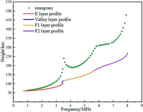
Figure 1. Examples of typical ionospheric electron density profile and ionogram.

According to the established electron density profile, we can calculate the reflected echo virtual height for each layer, which for O-wave traces can be expressed as Equation 7:

$h^{\prime }\left(f\right)={\int }_{h_0}^h{\mu }^{\prime }dh={\int }_{h_0}^h\frac{1}{1-X}dh={\int }_{h_0}^{h}1/\sqrt{1-f_n^2/f^2}dh(7)$

Bringing the electron density profile expression of Equation 6 into the integral relation yields (Equation 8):

$h^{\prime }\left(f\right)={\int }_{r_{bi}}^{r_{fi}}\begin{array}{c}\frac{rdr}{\sqrt{A_i{r}^2+B_{i}r+C_i}}\end{array}(8)$

$A_i=1-\frac{a_i}{f^2}+\frac{b_i}{f^2},B_i=-\frac{2b_i{r}_{mi}}{f^2},C_i=\frac{b_i{r}_{mi}^2}{f^2}$.

where the subscript $i$ denotes the different layers, representing layer E, valley, F1 and F2, respectively. Expanding the integral formula, the virtual height expression can be obtained as the following formula. The virtual height of layer $i$ is

$\begin{array}{c}{h}_i^{\prime }=\frac{1}{A_i}\left(\sqrt{A_i{r}_{fi}^2+B_i{r}_{fi}^2+C_i}-\sqrt{A_i{r}_{bi}^2+B_i{r}_{bi}+C_i}\right)\\ -\frac{B_i}{2\sqrt{A_i^3}}\mathit{lg}\left(\frac{2A_i{r}_{fi}+B_i+2\sqrt{A_i}\sqrt{A_i{r}_{fi}^2+B_i{r}_{fi}^2+C_i}}{2A_i{r}_{bi}+B_i+2\sqrt{A_i}\sqrt{A_i{r}_{bi}^2+B_i{r}_{bi}^2+C_i}}\right)\end{array}(9)$

The specific inversion process is as follows. Read each layer of the ionogram and generate k frequency points per layer, their corresponding operating frequencies and virtual height are respectively $f_k$ and $h^{″}\left(f_k\right)$, read the critical frequency and minimum virtual height of each layer as $f_{ci}$ and $h_{mini}^{″}$.

Then, set the value range of the three feature parameters $f_{ci}$, $h_{bi}$, $y_{mi}$ as [$f_{ci}$-0.2, $f_{ci}$ +0.2], [$h_{mini}^{″}$'-${\sigma }_1$, $h_{mini}^{″}$ + ${\sigma }_2$], [0, ${\sigma }_3$] (${\sigma }_1$, ${\sigma }_2$, and ${\sigma }_3$ are the searching range control quantities) at a certain step, respectively, and the three feature parameters can be obtained by taking the values within the set range to obtain many sets of feature parameter combinations. Each set of parameters is calculated according to Equation 9 to obtain $h^{\prime }\left(f_k\right)$ for k points, then calculate the error sum of squares of the measured virtual height, as shown in Equation 10:

$\epsilon ={\displaystyle \sum _1^k}{\left(h_k^{\prime }-h_k^{″}\left(f_c,r_m,y_m\right)\right)}^2(10)$

Here a method of global search is used, which results in finding a set of parameters $f_c$, $r_m$, $y_m$ such that ε is minimized.

According to the above inversion method, the electron density profile obtained from the inversion of the ionogram O-wave traces can be obtained, and we use this electron density profile as the background data for data assimilation.

3 Data assimilation methods and processes

3.1 Assimilation algorithm

Data assimilation refers to the integration of observational data into models based on physical laws. It integrates observational and modeled data, two different but complementary types of information, to improve the accuracy of analysis. The assimilation process can be viewed as an optimal combination of observational information and background models, grounded in error covariance matrices. Generally speaking, data assimilation primarily encompasses three aspects: (1) Observations and background values. Observations contain measurement and representativeness errors and are not exact values, so we use a variety of theories to estimate their true values as best we can; (2) Uncertainty. Errors themselves are also useful information in data assimilation, and how the assimilation process accounts for these errors ultimately determines the effectiveness of the assimilation. (3) Covariance. This essentially refers to the physical and spatial correlations between various values. For data assimilation, these correlations are themselves valuable information.

Data assimilation methods can be primarily categorized into two types based on their theoretical foundations: one type is estimation methods based on statistical theory, such as optimal interpolation and Kalman filtering; the other type comprises variational methods based on variational theory, such as three-dimensional variational assimilation. Currently, the Kalman filter method is the predominant approach used by major numerical forecasting centers (for example, JPL/USC GAIM) worldwide for data assimilation (Kalman, 1960; Kalman and Bucy, 1961; Scherliess et al., 2006). In this paper, we also adopt this method for data assimilation.

We use the vertical sounding ionogram X-mode virtual height traces as observational data for data assimilation. The X-mode virtual height $h_x^{\prime }$ of the ionogram is represented as the integral of the group refractive index along the real height of radio wave reflection, that is

$h_x^{\prime }\left(f\right)={\int }_{h_b}^{h_r}{\mu }_x^{\prime }dh(11)$

${\mu }_x^{\prime }$ denotes the group refractive index of the X-mode wave. According to magnetoplasma theory, the relationship between the group refractive index and the phase refractive index can be derived, which is expressed as follows:

${\mu }_x^{\prime }={\mu }_x+f\frac{d{\mu }_x}{df}(12)$

Equation 4 has already provided the expression for ${\mu }_x$. Expanding this equation further yields:

${\mu }_x+f\frac{d{\mu }_x}{df}={\mu }_x+f\frac{\partial X}{\partial f}\frac{\partial {\mu }_x}{\partial X}+f\frac{\partial Y}{\partial f}\frac{\partial {\mu }_x}{\partial Y}={\mu }_x-\left(2X\frac{\partial {\mu }_x}{\partial X}+Y\frac{\partial {\mu }_x}{\partial Y}\right)(13)$

where X = $f_n^2/f^2$, $f_n\left(h\right)$ is the electron density profile obtained by inversion of the O-wave traces. Substituting the aforementioned expanded expression into Equation 11 for integration yields the calculated virtual height of the X-mode wave. In particular, Equations 12, 13 calculate the group refractive index, and the calculated group refractive index is subsequently substituted into Equation 11 to obtain the calculated virtual height value of the X-wave.

In Equation 11, $h_x^{\prime }\left(f\right)$ represents the virtual height of the reflected echo corresponding to the operating frequency, $h_b$ denotes the bottom height of the ionosphere, $h_r$ is the real height of reflection at the operating frequency. Using the discretization inversion theory, the area to be assimilated is gridded in the height direction, and the above equation can be simplified to the following form:

$d=H{X}_b+e(14)$

In Equation 14, $d$ represents the observed ionogram X-mode virtual height trace, $H$ is the observation operator, which maps the background electron density to virtual height. Angling and Cannon (2004) provided a detailed exposition on $H$. $e$ denotes the discretization error, which is often neglected in its impact. Using Kalman filter theory, the data assimilation process for observational data can be expressed as:

$X_a=X_b+B{H}^T{\left[R+HB{H}^T\right]}^{-1}\left(d-\mathrm{H}{X}_b\right)(15)$

In Equation 15, $X_b$ represents the background value, which is the background electron density provided by the background ionospheric model; $X_a$ denotes the analysis value, which is the electron density obtained after assimilation; B and R represent the background error covariance and the observation error covariance, respectively. Based on the aforementioned formulas, we can view data assimilation as a process of correcting the background values using observations.

3.1.1 Observation error covariance

The ionosphere is complex and variable on both temporal and spatial scales; therefore, accurately characterizing observational errors is crucial. Previous studies, such as Angling and Cannon (2004) have assumed during data assimilation that the observational errors (background errors) are proportional to the square of the corresponding observational values and that the observational errors are unbiased and mutually independent. We also adopt this assumption, where the observational error is represented as the product of a proportionality coefficient and the square of the observational value. Clearly, the observational error covariance should be a diagonal matrix, with the diagonal elements being the product of the proportionality factor and the square of the observational values. It can be expressed as follows:

$R_{ij}={\sigma }_i{\sigma }_j{\rho }_{ij}=\left\{\begin{array}{l}{\eta }_0{Y}_i{Y}_j\left({\rho }_{ij}=1,i=j\right)\\ 0,\left({\rho }_{ij}=0,i\ne j\right)\end{array}\right.(16)$

In Equation 16, $i,\mathrm{j}$ indicate observation points; $R_{ij}$ is the covariance of errors between observation points; ${\eta }_0$ is the proportionality coefficient, ${\rho }_{ij}$ is the correlation coefficient, the correlation coefficient between different observation points is 0, $Y_i$ represents the observation value of the observation point. In this paper, the observational values are the virtual height of the X wave from the ionogram, $Y_i$ denoted as representing the virtual height value of the X wave at point $i$.

In previous studies, a uniform proportionality factor was often employed, which can introduce significant errors as it fails to accurately and effectively describe the variations in the ionosphere. This study employs data from ionospheric vertical sounding stations for statistical analysis to derive the proportionality coefficients. Specifically, we utilize the values of the ionosphere recorded by the Wuhan vertical sounding station from June 1st to 30 June 2021, at 11:00 each day. The ionospheric region between 100 and 300 km in altitude is gridded with a vertical height direction, and the interval between grids is 4 km. Taking the monthly average virtual height as the reference value, we statistically analyze the daily deviations of the ionospheric vertical sounding virtual height values from the reference at that moment. Then, the squared observations are linearly fitted with the observation errors, and the fitting coefficients are provided. Figure 2 shows the curve of the mean observed virtual height as a function of frequency. Figure 3 shows the fitted relationship between the square of the observed virtual height and the observation error.

Figure 2

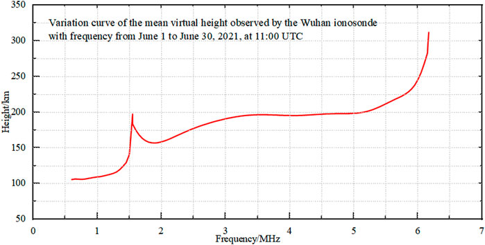
Figure 2. Variation of the mean virtual height with frequency of o-wave traces observed by the Wuhan Ionosonde from June 1 to 30 June 2021 at 11:00.

Figure 3

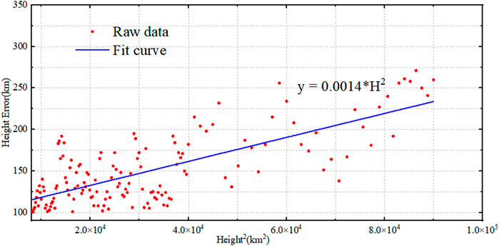
Figure 3. The variation of observation errors from the Wuhan ionosonde with the square of the corresponding observed virtual heights, along with the fitting curve, at 11:00 from June 1st to 30 June 2021.

3.1.2 Background error covariance

The background error covariance matrix is crucial for ionospheric data assimilation. It is primarily composed of two parts: the variance of the background model used for assimilation and the correlation between the model’s errors at any two grid points. For each element of the error covariance matrix, we can express it with the following Equation 17:

$B_{ij}={\sigma }_i{\sigma }_j{\rho }_{ij}(17)$

${\sigma }_i$, ${\sigma }_j$ are the standard deviations of the forecast model at the ith and jth grid points, respectively, and ${\rho }_{ij}$ is the linear correlation coefficient between these errors.

Drawing on previous literature (Angling and Cannon, 2004; Bust et al., 2004; Forsythe et al., 2020; Forsythe et al., 2021a; Yue et al., 2012; Yue et al., 2011), we assume that the background field is Gaussian distributed and can be Gaussianly separated in both horizontal (latitude and longitude) and vertical directions. At the same time, our observations and background data consist of virtual height and electron density profiles, so we only need to consider the vertical direction.

Regarding the vertical correlation ${\rho }_{ij}$, previous studies (Bust et al., 2004; Angling Cannon, 2004) typically describe it using the following expression using Equation 18:

${\rho }_{ij}=e^{-\left(r_{ij}^2/2L^2\right)}(18)$

$r_{ij}$ represents the distance between any two grid points, and $L$ is the vertical correlation distance, which is typically taken as a fixed constant. However, this approach introduces certain errors. Later, Forsythe et al. (2021a) conducted an in-depth analysis of vertical correlation using various observational data and provided a more accurate definition, which is expressed as the following Equation 19:

${\rho }_{ij}=\left\{\begin{array}{l}\mathit{exp}\left[-\frac{{\left(Z_i-Z_j\right)}^2}{{\left(L_1\left(Z_i,{\lambda }_i\right)\right)}^2}\right]Z_i<Z_j\\ \mathit{exp}\left[-\frac{{\left(Z_i-Z_j\right)}^2}{{\left(L_2\left(Z_i,{\lambda }_i\right)\right)}^2}\right]Z_i>Z_j\\ 1Z_i=Z_j\end{array}\right.(19)$

In this context, Z represents the altitude, $\lambda$ denotes the magnetic latitude, and $L_1$, $L_2$ are the vertical correlation lengths, which are functions of geomagnetic latitude and altitude, respectively. These variables can be found in the databases constructed by Forsythe et al. (2020). The method proposed by Forsythe et al. (2021a) provides a more rational definition of the vertical correlation distance; therefore, this paper adopts their approach to construct the vertical correlation matrix of the background error covariance. The flow chart of the assimilation algorithm is depicted in Figure 4.

Figure 4

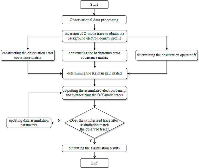
Figure 4. Flow chart of the data assimilation algorithm.

4 Results and analysis

Based on an extensive dataset recorded (it contains 17,568 ionograms) from vertical soundings in the Wuhan area, we validated the inversion algorithm. In this section, we present several typical ionograms to illustrate the effectiveness of the algorithm. For each set of figures, we provide the background electron density profile and its synthesized O/X wave virtual height traces, the profile inverted by the Reinisch algorithm and its synthesized virtual height traces, as well as the electron density profile obtained after assimilation and its synthesized virtual height traces. In each subplot, the black hollow circles represent the observed X-wave traces on the ionogram, the black hollow squares indicate the observed O-wave traces, the blue solid or dashed lines depict the electron density profiles, the red solid line is the O-wave virtual height trace synthesized from the integration of the group refractive index ${\mu }^{\prime }$ after assimilation, and the green solid line is the X-wave virtual height trace synthesized from the integration of the group refractive index ${\mu }^{\prime }$ post-assimilation. We compared the X-wave virtual height traces synthesized from the profiles obtained after assimilation analysis with those synthesized from the profiles inverted by the Reinisch algorithm and presented the distribution histogram of the errors. The mean and variance are defined as Equations 20, 21:

$\mu \left(∆h^{\prime }\right)={\displaystyle \sum _{i=1}^N}\left|h^{\prime }\left(f_i\right)-h^{″}\left(f_i\right)\right|/N(20)$

$\sigma \left(∆h^{\prime }\right)=\sqrt{{\displaystyle \sum _{i=1}^N}{\left(∆h_{\left(i\right)}^{\prime }-∆\overline{h}\right)}^2/N}(21)$

We gridded the ionosphere along the vertical height, where $i$ denotes the corresponding grid point, $h^{\prime }\left(f_i\right)$ represents the observed virtual height at the $i$-th grid point, $h^{″}\left(f_i\right)$ represents the virtual height synthesized from the electron density after assimilation at the $i$-th grid point, $\mu \left(∆h^{\prime }\right)$ denotes the average virtual height error of N grid points, $∆\overline{h}$ represents the average virtual height error, $∆h_{\left(i\right)}^{\prime }$ indicates the error between the observed virtual height and the synthesized virtual height at the $i$-th grid point, and $\sigma \left(∆h^{\prime }\right)$ signifies the variance of the error values. The horizontal axis of the histogram represents the differences between the virtual height synthesized from the integral of electron density at each grid point and the observed virtual height. The vertical axis represents the cumulative number of grid points corresponding to the virtual height error differences.

Figure 5 illustrates a two-layer ionogram where the F1 layer is absent. As can be seen from Figure 5A, the O-wave trace synthesized from the background electron density profile aligns well with the actual measured trace (the mean fitting error of the synthesized O-wave traces to the measured traces is 2.86 km); however, the synthesized X-wave trace shows a poor fit with the actual measured trace (the mean value of the fitting error between the synthetic x-wave traces and the measured traces is 10.64 km). In Figure 5B, the X-wave trace synthesized from the profile inverted by the Reinisch algorithm exhibits a significant discrepancy with the actual measured trace, particularly in the region where the E-layer connects with the F-layer (the frequency range between 3.5 MHz and 3.9 MHz corresponds to the height region in the figure). The synthesized X-wave trace from the inverted profile is considerably larger than the actual measured trace. The electron density profile obtained using the joint inversion method of O-wave and X-wave is displayed in Figure 5C. It can be observed that the synthesized X-wave trace from the profile after assimilation analysis aligns well with the actual measured trace. Although the synthesized O-wave trace at this point does not fit the actually measured trace as well as the profiles obtained from the first two algorithms, the synthesized X-wave trace shows a significant improvement in fitting the actual X-wave trace. Overall, there is a noticeable reduction in the error compared to the actual measured traces of both O-wave and X-wave. In the histogram of error distribution (Figure 5D), the mean error of the profile synthesized by the Reinisch algorithm inversion is 8.639 km, and the variance is 18.316 km. After data assimilation, the mean error of the profile synthesized by the analysis is 3.256 km, and the variance is 3.258 km. This indicates that increasing the inversion data can effectively improve the accuracy of the inversion.

Figure 5

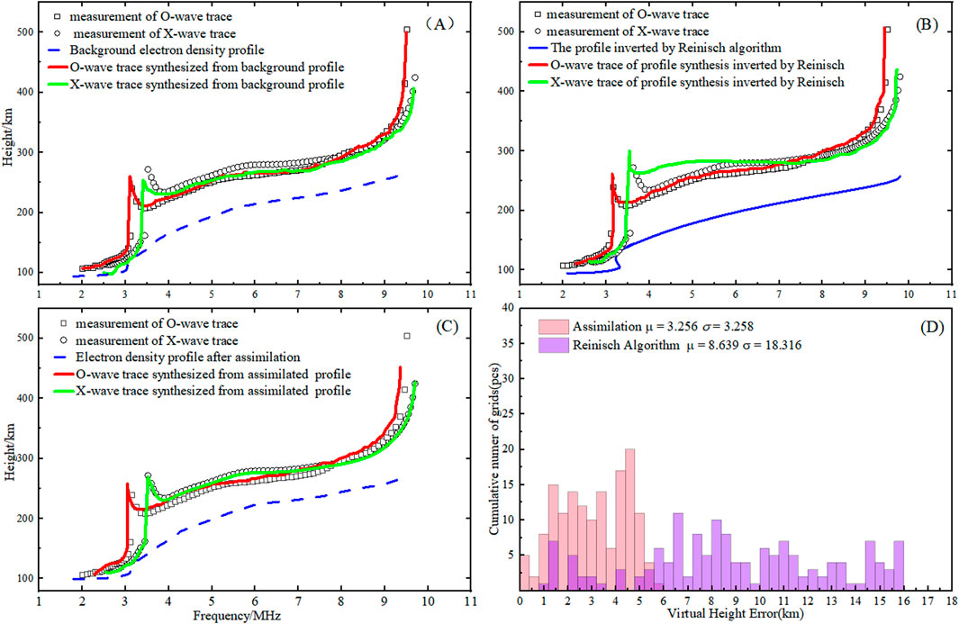
Figure 5. Observation of O/X mode traces in ionograms (June 1, 2021, LAT:30.6, LON:114.6, 12:24 UTC). (A) Background electron density profiles and their synthetic traces. (B) Reinisch algorithm inversion profile and its synthetic tracing. (C) Assimilated electron density and its synthetic traces. (D) Error distribution statistics before and after assimilation.

Figure 6 presents a typical three-layer ionogram. Observing this actual measurement trace, it is evident that the O-wave trace synthesized from the background electron density profile aligns well with the measured data. However, the correspondence of the X-wave trace is less satisfactory, particularly in the F1-layer, where the simulated elevated trace diverges significantly from the empirical observations. Moreover, the virtual height traces synthesized from the electron density profiles obtained through the joint inversion method using both O-wave and X-wave exhibit a high degree of consistency with the measured traces. As illustrated by the error distribution histogram, the application of the Reinsch algorithm has led to an improvement in the profile inversion accuracy, with the mean error decreasing from 7.81 km to 4.32 km.

Figure 6

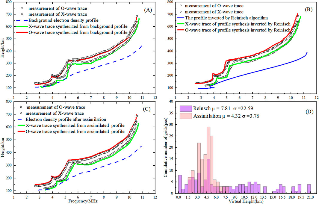
Figure 6. Observation of O/X mode traces in ionograms (June 12, 2021, LAT:30.6, LON:114.6, 13:42 UTC). (A) Background electron density profiles and their synthetic traces. (B) Reinisch algorithm inversion profile and its synthetic tracing. (C) Assimilated electron density and its synthetic traces. (D) Error distribution statistics before and after assimilation.

Figure 7 is also a three-layer type ionogram. In Figure 7A, the synthetic virtual height traces derived from the background electron density profile differ significantly from the measured traces in the F1 and F2 layer regions. However, the synthesized O-wave trace shows a good match with the measured data. This is because the background electron density profile is a least-squares fit to the measured data. The O-wave and X-wave traces synthesized from the electron density profile inverted using the Reinisch algorithm exhibit significant errors when compared to the measured traces. It is observed that after assimilation analysis, the synthesized X-wave trace shows improved fitting with the measured trace. Relative to the synthesized traces in Figure 7A, the fitting quality of the O-wave trace synthesized from the assimilated profile deteriorates. Despite this, the overall fitting situation for both the O-wave and X-wave traces is better.

Figure 7

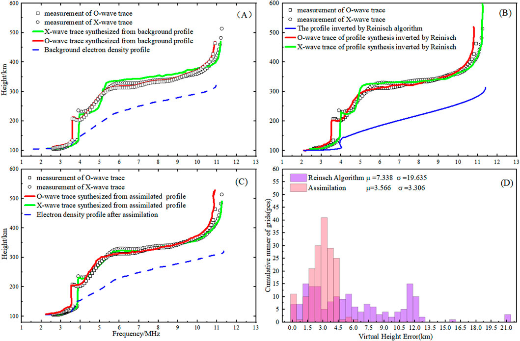
Figure 7. Observation of O/X mode traces in ionograms (June 25, 2021, LAT:30.6, LON:114.6, 11:32 UTC). (A) Background electron density profiles and their synthetic traces. (B) Reinisch algorithm inversion profile and its synthetic tracing. (C) Assimilated electron density and its synthetic traces. (D) Error distribution statistics before and after assimilation.

In order to further verify the feasibility and effectiveness of the algorithm, we used a large number of continuously observed ionogram data for testing (it contains 576 ionograms). Figure 8 shows the results of the analysis using actual ionograms obtained on 2 May 2021, from the Wuhan station. Figure 8A represents the original ionogram traces, i.e., the true values; Figure 8B is the ionogram traces synthesized from the electron density profiles based on the inversion of the background model; and Figure 8C is the ionogram traces synthesized from the electrons density after the joint inversion by O-wave and X-wave.There is a clear difference between Figures 8A, B, especially during the period from 8 a.m. to 3 p.m. (the local time). During this time period, due to sufficient solar radiation, the ionosphere is sufficiently ionized, producing a large number of free electron. Therefore, the detected ionograms are complete and there are significant differences in the virtual height corresponding to different frequencies, which is manifested in the large color differences in the height corresponding to different frequencies in the Figure.

Figure 8

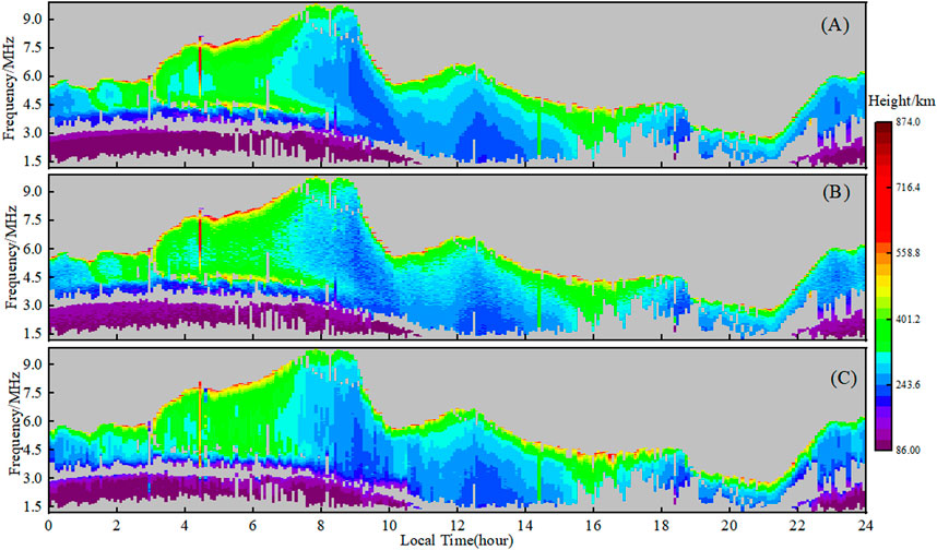
Figure 8. Results of the joint inversion of the continuously observed ionograms (May 2, 2021, LAT:30.6, LON:114.6). (A) Continuous measured ionogram traces. (B) Synthesized ionograms of background electron density profiles. (C) synthetic ionograms of assimilated electron density profiles.

Therefore, during this period, the profile inverted by the background ionospheric model using only O-wave traces cannot accurately reflect the true electron density distribution, and there is a certain deviation between the synthesized traces and the true traces. Using the joint O-wave and X-wave inversion algorithm proposed in this paper (shown in Figure 8C), the X-wave traces are introduced into the inversion, which in turn go on to correct the electron density profiles obtained from the background model inversion. It can be seen that the concordance between the synthesized ionogram traces and the true traces is significantly improved, indicating that the electron density profiles obtained by the joint inversion are closer to the true electron density distribution. Moreover, the traces synthesized from the jointly inverted profiles Figure 8C and the traces synthesized from the background model inverted profiles Figure 8B are essentially the same in the region of frequencies below 3 MHz and height below 150 km, and they are in almost perfect accordance with Figure 8A.

This is because the height range belongs to the E-layer of the ionosphere, where the electron density is relatively flat, and the profiles obtained by the background model based on the inversion of the O-wave traces in the E-layer are already very close to the true electron density distribution, thus both the background model and the results obtained by the joint inversion method have less variations and higher consistency.

Similarly, Figure 9 shows the results of the detection analysis at Wuhan station on 21 June 2021, with Figure 9A showing the traces of the measured true ionogram, Figure 9B showing the traces synthesized by the inversion profiles of the background model, and Figure 9C showing the traces synthesized by the profiles of the joint inversion. Similarly, it can be observed that in the time period of 5:00-14:00 (belonging to the summer season), the traces synthesized by the profiles of the background model inversion, i.e., Figure 9B, are somewhat different from the true ionogram traces, Figure 9A, due to the reason similar to that of Figure 8, which is that there is a large variation of the electron density and a higher F2 layer peak during the time period, and it is difficult for the profiles synthesized by the background model inversion to closely approximate the true electron density distribution. Therefore, Figure 9B has some differences with Figure 9A, whereas the traces synthesized from the profiles we inverted using the joint O\X-wave inversion, i.e., Figure 9C, are less different from the true traces, i.e., Figure 9A, which again shows that the electron density profiles obtained by the joint inversion are more similar to the true electron density profile, and have a better consistency.

Figure 9

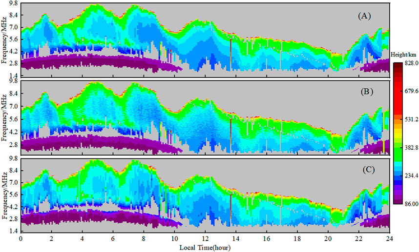
Figure 9. Results of the joint inversion of the continuously observed ionograms (June 21, 2021, LAT:30.6, LON:114.6). (A) Continuous measured ionogram traces. (B) Synthesized ionograms of background electron density profiles. (C) synthetic ionograms of assimilated electron density profiles.

5 Conclusion

This paper presents a method for inverting ionospheric electron density profiles based on the assimilation and inversion of O/X-wave traces from vertical sounding ionograms. In this study, we use the electron density profiles inverted from O-wave traces as background data and the X-wave traces from ionograms as observational data. By employing the Kalman filter method, we perform joint inversion of O-wave and X-wave trace data to obtain more accurate electron density profiles. Through comparative analysis of the O-wave and X-wave traces synthesized from the inverted electron density profiles with the corresponding measured traces, it was found that while the synthetic O-wave traces derived from the assimilated profiles show slightly less agreement with the measured traces, the synthetic X-wave traces exhibit good fit with the measured traces. Overall, this approach significantly reduces the errors between the synthetic and measured O-wave and X-wave traces, thereby effectively improving the accuracy of the inverted profiles.

The joint inversion method proposed in this study is not only theoretically clear but also practical and feasible in real-world applications, demonstrating considerable potential value. Future research directions will focus on integrating additional physical measurement information to further enhance the accuracy of the inversion algorithm for vertical sounding ionograms. Such improvements are expected to provide more reliable electron density distribution data for ionospheric studies, thus promoting deeper developments in related fields.

Data availability statement

Publicly available datasets were analyzed in this study. This data can be found here: China National Meridian Project Data Center, www.meridianproject.ac.cn.

Ethics statement

Ethical approval was not required for the study involving humans in accordance with the local legislation and institutional requirements. Written informed consent to participate in this study was not required from the participants or the participants’; legal guardians/next of kin in accordance with the national legislation and the institutional requirements.

Author contributions

LN: Conceptualization, Data curation, Formal Analysis, Investigation, Methodology, Project administration, Software, Supervision, Validation, Visualization, Writing–original draft, Writing–review and editing. CZ: Visualization, Writing–review and editing, Conceptualization, Data curation, Project administration. NW: Visualization, Writing–review and editing, Formal Analysis, Software, Supervision. Z-XD: Supervision, Validation, Writing–review and editing. YN: Formal Analysis, Methodology, Writing–review and editing. RC: Formal Analysis, Methodology, Validation, Visualization, Writing–review and editing. WL: Conceptualization, Formal Analysis, Funding acquisition, Investigation, Project administration, Resources, Software, Visualization, Writing–review and editing.

Funding

The author(s) declare that financial support was received for the research, authorship, and/or publication of this article. This work was supported by the National Key Research and Development Program of China (No. 2023YFA1009100).

Conflict of interest

The authors declare that the research was conducted in the absence of any commercial or financial relationships that could be construed as a potential conflict of interest.

Generative AI statement

The author(s) declare that no Generative AI was used in the creation of this manuscript.

Publisher’s note

All claims expressed in this article are solely those of the authors and do not necessarily represent those of their affiliated organizations, or those of the publisher, the editors and the reviewers. Any product that may be evaluated in this article, or claim that may be made by its manufacturer, is not guaranteed or endorsed by the publisher.

References

Anderson, J., Hoar, T., Raeder, K., Liu, H., Collins, N., Torn, R., et al. (2009). The data assimilation research testbed: a community facility. Bull. Am. Meteorol. Soc. 90, 1283–1296. doi:10.1175/2009bams2618.1

CrossRef Full Text | Google Scholar

Angling, M. J., and Cannon, P. S. (2004). Assimilation of radio occultation measurements into background ionospheric models. Radio Sci. 39, RS1S08. doi:10.1029/2002rs002819

CrossRef Full Text | Google Scholar

Bilitza, D., Pezzopane, M., Truhlik, V., Altadill, D., Reinisch, B. W., and Pignalberi, A. (2022). The international reference ionosphere model: a review and description of an ionospheric benchmark. Rev. Geophys. 60, e2022RG000792. doi:10.1029/2022rg000792

CrossRef Full Text | Google Scholar

Bust, G. S., Garner, T. W., and Gaussiran, T. L. (2004). Ionospheric data assimilation three-dimensional (IDA3D): a global, multisensor,electron density specification algorithm. J.Geophys. Res. Space Phys. 109, A11312. doi:10.1029/2003ja010234

CrossRef Full Text | Google Scholar

Croft, T. A., and Hoogasian, H. (1968). Exact ray calculations in a quasi-parabolic ionosphere with no magnetic field. Radio Sci. 3 (1), 69–74. doi:10.1002/rds19683169

CrossRef Full Text | Google Scholar

Dyson, P. L., and Bennett, J. A. (1988). A model of the vertical distribution of the electron concentration in the ionosphere and its application to oblique propagation studies. J. Atmos. Terr. Phys. 50 (3), 251–262. doi:10.1016/0021-9169(88)90074-8

CrossRef Full Text | Google Scholar

Forsythe, V. V., Azeem, I., Blay, R., Crowley, G., Gasperini, F., Hughes, J., et al. (2021a). Evaluation of the new background covariance model for the ionospheric data assimilation. Radio Sci. 56, e07286. doi:10.1029/2021rs007286

CrossRef Full Text | Google Scholar

Forsythe, V. V., Azeem, I., and Crowley, G. (2020). Ionospheric horizontal correlation distances: estimation, analysis, and implications for ionospheric data assimilation. Radio Sci. 55 (12), 1–14. doi:10.1029/2020rs007159

CrossRef Full Text | Google Scholar

He, J., Yue, X., Wang, W., and Wan, W. (2019). EnKF ionosphere and thermosphere data assimilation algorithm through a sparse matrix method. J. Geophys. Res. Space Phys. 124, 7356–7365. doi:10.1029/2019ja026554

CrossRef Full Text | Google Scholar

Kalman, R. E. (1960). A new approach to linear filtering and prediction problems. J. Basic Eng. 82, 35–45. doi:10.1115/1.3662552

CrossRef Full Text | Google Scholar

Kalman, R. E., and Bucy, R. (1961). New results in linear filtering and prediction theory. J. Basic Eng. 83, 95–108. doi:10.1115/1.3658902

CrossRef Full Text | Google Scholar

Mengist, C. K., Ssessanga, N., Jeong, S.-H., Kim, J.-H., Kim, Y. H., and Kwak, Y.-S. (2019). Assimilation of multiple data types to a regional ionosphere model with a 3D-var algorithm (IDA4D). Space weather. 17, 1018–1039. doi:10.1029/2019sw002159

CrossRef Full Text | Google Scholar

Niu, L., Wen, L., Zhou, C., and Deng, M. (2024). A profile inversion method for vertical ionograms. AIP Adv. 14 (6). doi:10.1063/5.0208687

CrossRef Full Text | Google Scholar

Reinisch, B. W., and Huang, X. (1983). Automatic calculation of electron density profiles from digital ionograms: 3. Processing of bottomside ionograms. Radio Sci. 18, 477–492. doi:10.1029/rs018i003p00477

CrossRef Full Text | Google Scholar

Scherliess, L., Schunk, R. W., Sojka, J. J., Thompson, D. C., and Zhu, L. (2006). Utah state university global assimilation of ionospheric measurements gauss-markov Kalman filter model of the ionosphere: model description and validation. J. Geophys. Res. Space Phys. 111, A11315. doi:10.1029/2006ja011712

CrossRef Full Text | Google Scholar

Spencer, P. S., Robertson, D. S., and Mader, G. L. (2004). “Ionospheric data assimilation methods for geodetic applications,” in PLANS 2004. Position location and navigation symposium. IEEE Cat. No. 04CH37556, 510–517.

Google Scholar

Titheridge, J. E. (1967). The overlapping-polynomial analysis of logograms. Radio Sci. 2, 1169–1175. doi:10.1002/rds19672101169

CrossRef Full Text | Google Scholar

Yue, X., Schreiner, W. S., Kuo, Y. H., Hunt, D. C., Wang, W., Solomon, S. C., et al. (2012). Global 3-D ionospheric electron density reanalysis based on multisource data assimilation. J. Geophys. Res. Space Phys. 117 (A9). doi:10.1029/2012ja017968

CrossRef Full Text | Google Scholar

Yue, X., Schreiner, W. S., Lin, Y.-C., Rocken, C., Kuo, Y.-H., and Zhao, B. (2011). Data assimilation retrieval of electron density profiles from radio occultation measurements. J. Geophys. Res. Space Phys. 116, A03317. doi:10.1029/2010ja015980

CrossRef Full Text | Google Scholar