The role of the dynamic terrestrial exosphere in the storm-time ring current decay

The charge exchange interaction between exospheric hydrogen (H) atoms and energetic ions in the terrestrial ring current is a crucial mechanism for dissipating global magnetospheric energy, especially during the recovery phase of geomagnetic storms. Historically, ring current modeling has considered H density distributions temporally static and spherically symmetric owing to the lack of event-specific exospheric models. However, observations of the far-ultraviolet (FUV) emission from exospheric H atoms acquired by NASA’s TWINS Lyman-Alpha Detectors (LADs) unveiled not only spatial asymmetries but also significant temporal variability of this neutral population, particularly during storm time. In this work, we investigate the influence of realistic exospheric H density distributions on the ring current decay during the strong storm on 1 June 2013. To do so, we first estimate time-dependent, three-dimensional (3-D) H density distributions using FUV radiance data acquired by TWINS/LADs with a robust tomographic approach. Then, we use these neutral distributions as inputs for the Comprehensive Inner Magnetosphere-Ionosphere (CIMI) model and simulate the ion ring current behavior as a response to the exospheric dynamics. We compared the resulting ion fluxes with those produced when a static and spherically symmetric H model (Rairden's model) is used. We found that the TWINS-based global hydrogen density beyond 3 $R_E$ geocentric distances is, on average, $\sim 35\%$ larger than that of Rairden’s model during quiet time and increases up to $\sim 50\%$ during the geomagnetic storm. Consequently, the ring current ion flux during the recovery phase decays faster when the TWINS-based model is used. Our comparison study shows that using a realistic H-density model produces $\sim$60% lower ion fluxes (${\text{H}}^{+}$ and ${\text{O}}^{+}$ with energy range 0.1–60 keV) than those yielded by Rairden’s model, especially during the recovery phase and at $L$-shells $<$4 $R_E$. Also, when the TWINS-based model is used, the total ring current energy during the recovery phase is $\sim$30% lower than the energy calculated with the static exospheric model.

1 Introduction

The outermost region of the Earth’s atmosphere is known as the exosphere and extends beyond several hundreds of kilometers ($\sim$500 km) up to the Moon ($\sim$ 60 Earth radii $(R_E)$) (Baliukin et al., 2019). It mainly comprises neutral hydrogen atoms (H), which scatter solar FUV emissions, forming a bright, gravitationally-bound cloud known as the “geocorona”. Due to its vast extension, the terrestrial exosphere is embedded with several plasma populations, such as the plasmasphere, ring current, and plasma sheet in the inner magnetosphere, as well as the magnetosheath and solar wind in the outer magnetosphere, each of them featuring a particular spatial location and energy distribution. Interactions between the neutral and plasma populations occur constantly via charge exchange, in which an energetic ion picks up the electron of an exospheric H atom, forming a cold ion and an energetic neutral atom (ENA). These ENAs are not affected by electric or magnetic fields and may escape to interplanetary space (Ilie et al., 2012).

Previous studies demonstrated the crucial role of the exosphere in inner magnetospheric dynamics due to charge exchange interactions. Early in the space exploration era, observational and theoretical studies of the near-Earth plasma environment linked the strength of geomagnetic storms to the development of the terrestrial ring current, and its recovery to quiet-time conditions was associated with the transfer of energy from ring current ions to exospheric H atoms via charge exchange (Dessler and Parker, 1959). Since then, numerous studies have stated the critical role of the spatial density distribution of the neutral population in ring current dynamics, especially in the decay phase [(Jordanova, 2020); and references therein]. Because the exospheric H density decreases with increasing radial distance, the effects of charge exchange are larger, and its role in defining the ring current distribution is more important at low L shells. Moreover, since the ring current is composed of a variety of ion species, each having distinct charge exchange timescales (i.e., cross sections), their interactions with exospheric atoms highly affect not only the overall ring current decay evolution but also its ion composition and redistribution. This particular effect was shown by measurements that reported heavy ions dominating over the overall most abundant protons at the low L shells near the inner edge of the ring current (Ferradas et al., 2015; Ferradas et al., 2016; Kistler et al., 1989; Kistler et al., 1998; Lundin et al., 1980). This was well explained by the significantly longer charge exchange lifetimes of heavy ions compared to those of protons at those energies.

With more emphasis on the variability of the geocoronal population, Krall et al. (2018) conducted a study to evaluate the impact of atomic H on the temporal rates of plasmaspheric refilling and ring current recovery after a geomagnetic storm. They pointed out the prevailing uncertainty of the current knowledge of exospheric densities and tested plasmasphere and ring current models using H concentrations derived from the NRLMSIS (Emmert et al., 2021; Rairden et al., 1986) H models, which included multiplicative factors of 0.5 and 2 supported by preceding data-based comparison studies (Waldrop and Paxton, 2013; Nossal et al., 2012; Kotov et al., 2023). The results showed that a fast ring current recovery rate is highly associated with large exospheric H densities.

A specific investigation on the impact of geocoronal densities on ring current dynamics has been previously conducted by Ilie et al. (2013). For this purpose, they used a kinetic model known as the Hot Electron Ion Drift Integrator (HEIDI) to simulate ion dynamics in the ring current, as well as several state-of-the-art models of the terrestrial exosphere, which are briefly described here since it is pertinent to our study. 1) Hodges (1994) implemented a Monte-Carlo simulation of the exosphere that simulates atomic H dynamics from its origin in the middle thermosphere and its path towards the exosphere following ballistic, escaping, and satellite trajectories. The model considers ion-neutral interactions with various plasma populations, e.g., topside ionosphere, plasmasphere, and polar wind. 2) Rairden et al. (1986) estimated a spherically symmetric model of the exosphere based on an isothermal distribution of H atoms (Chamberlain, 1963) and measurements of the scattered Lyman-alpha (Ly-$\alpha$ at 121.6 nm) emissions acquired by the ultraviolet imaging photometer on the Dynamics Explorer 1 mission during 1983–1985.3) Bailey and Gruntman (2011) estimated a 3-D exospheric model based on parametric fitting to spherical harmonics that uses single-day (11 June 2008) measurements of Ly-$\alpha$ emission acquired by Lyman-Alpha Detectors (LADs) on board NASA’s Twins-Wide angle Imaging Neutral-atom Spectrometers (TWINS) mission. 4) Similarly, Zoennchen et al. (2015) reconstructed the 3-D exosphere using spherical harmonic functions and multi-day Ly-$\alpha$ observations from TWINS/LADs for solar minimum (June 2008) and solar maximum (October-December 2012) conditions. The use of these models as inputs in HEIDI certainly demonstrated the strong dependence of the resulting ring current ion flux on the 3-D exospheric density distributions. However, the storm event selected in this study occurred in July 2009, and H models (named 2, 3, and 4 above) were implemented using radiance data for other dates. Therefore, these models do not represent the actual structure of the exosphere, as the neutral population highly depends on the current solar conditions and geomagnetic activity.

Recently, Zoennchen et al. (2024) determined the 3-D structure of exospheric H density distributions using multi-day observations of TWINS/LADs instruments for both solar minimum and maximum conditions. It was found that the exosphere during solar maximum is $\sim$ 35% denser than in solar minimum at ring current altitudes ($\sim 2$ to $5R_E$). In both cases, the exosphere exhibits an asymmetric structure with a high H density near the dayside subsolar region and the nightside along the Sun-Earth line, which is an expected effect of solar radiation pressure (Beth et al., 2016). Regarding the effect of geomagnetic activity on the exospheric structure, Zoennchen et al. (2017) conducted a comparison analysis of TWINS/LAD radiance data acquired during several storms spanning weak, moderate, and strong types, resulting in enhancements of the H density beyond $2R_E$ altitudes. Based on this work, Cucho-Padin and Waldrop (2019) studied the 3-D time-dependent response of the exosphere during the weak storm that occurred on 15 June 2008, using TWINS/LAD data. They found global enhancements of H density in the main phase of the storm of $\sim$ 25% with respect to quiet-time conditions.

To quantify the effect of a realistic exospheric H density in ring current dynamics, this research work presents a comparative study between simulations of the ring current ion distributions during a geomagnetic storm using two exospheric models: a data-based model derived from actual TWINS emission data and the spherically symmetric and temporally static Rairden et al. (1986) model. In addition, these ion flux results are compared with in situ measurements acquired by the Van Allen Probes mission. This manuscript is organized as follows. Section 2 describes the event selected for this study, the remote sensing techniques to estimate H density from FUV emissions, and the model to simulate ring current ion dynamics. Section 3 presents the two ring current simulation results and the comparison between ion fluxes and total ring current energy during the evolution of the storm. Also, this section shows the comparison of these results with in situ observations from Van-Allen Probes. Finally, Section ?? discusses the results of our study and lists our conclusions.

2 Event description, data, and methods

2.1 Event overview

This study analyzes the intense geomagnetic storm that was triggered by the arrival of a coronal mass ejection (CME) and began with a sudden commencement on 1 June 2013, around 0300 UT, with a main phase that lasted for about 6 h until $\sim$0900 UT, followed by a long recovery phase that extended over at least 4 days. This storm has been selected due to the coincident availability of data from TWINS/LAD, which is needed to estimate exospheric H distributions, and Van Allen Probes instruments used to perform data-model comparisons. Figure 1 shows an overview of the geomagnetic activity, global thermospheric/exospheric conditions, and interplanetary environment during the storm’s development. Panels from top to bottom show the time series of (a) the horizontal component asymmetry index (SYM-H), (b) the globally-averaged exobase temperature $(T_{\mathit{exo}})$, (c) the globally-averaged exobase density $(n_{\mathit{Hexo}})$, and (d) the planetary K-index (Kp). Values from panels (b) and (c) were obtained from the National Center for Atmospheric Research (NCAR) Whole Atmosphere Community Climate Model with thermosphere and ionosphere extension (WACCM-X). The gray-shaded interval corresponds to the period of study in which the ring current is simulated and the terrestrial exosphere is estimated from NASA’s TWINS radiance data.

Figure 1

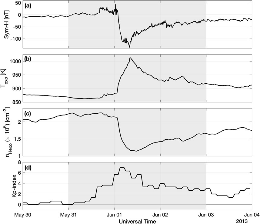
Figure 1. Overview of the intense geomagnetic storm on 1 June 2013. Panels from top to bottom indicate (a) SYM-H, (b) globally-averaged exobase temperature $(T_{\mathit{exo}})$, (c) globally-averaged exobase H density $(n_{\mathit{Hexo}})$, (d) planetary K-index (Kp). The gray-shaded interval corresponds to the period of study in which the ring current is simulated, and the terrestrial exosphere is estimated from NASA’s TWINS FUV data.

The variability of exospheric densities at ring current altitudes during a geomagnetic storm is typically associated with the global distribution and temporal variability of the temperature and densities at the exobase ($\sim$500 km) Chamberlain (1963). During the storm’s development, ion precipitation slowly increases the thermospheric temperature via the Joule heating process, propagating heat from the poles to the equator (Zesta and Oliveira, 2019). Light H atoms are highly sensitive to these temperature variations, resulting in a density re-distribution where atomic H density decreases near the exobase ($\sim$500 km altitude) and increases at high altitudes (ring current region) (Qin et al., 2017). This anti-correlation between density and temperature at the exobase is shown in panels (b) and (c). Furthermore, the energy partition of exospheric H atoms is continuously altered by plasmaspheric ions via charge exchange interactions, especially by protons (${\text{H}}^{+}$) with an energy range of $\sim 1-$2 eV. During geomagnetic storms, the plasmaspheric density decreases, and its external boundary, the plasmapause, moves inward, thus reducing the rate of charge exchange and varying the 3-D structure of the exosphere (Kuwabara et al., 2017). Panel (d) shows the Kp index, which is linearly correlated to the plasmapause location (Moldwin et al., 2002) and serves as another indicator of exospheric density variability.

2.2 Lyman-Alpha observations

We estimate global exospheric densities using radiance data from the TWINS mission. NASA’s TWINS is comprised of two spacecraft, TWINS1 and TWINS2, each of them featuring a highly elliptical orbit, an apogee in the Northern ecliptic hemisphere of 7.2 $R_E$ geocentric distance, and an orbital precession of 1 year. Each satellite has two Lyman-Alpha Detectors, LAD1 and LAD2, able to acquire FUV photon flux with a central wavelength of 121.6 nm (Ly-$\alpha$) (McComas et al., 2009). The LADs are single-pixel optical sensors with a 4$°$ field-of-view (FOV) assembled on a rotating platform in the spacecraft. Due to its geometrical configuration, the LADs acquire column-integrated photon flux measurements above $\sim$2 $R_E$ geocentric distance every $\sim$0.66 s.

To analyze the storm that occurred on 1 June 2013, we use radiance data acquired by LAD1/2 onboard the TWINS1 spacecraft for 3 days from May 31 to June 2. The LADs onboard TWINS2 were out of commission after 2012.

2.3 Tomographic reconstructions of dynamic exospheric density distributions

In this study, we estimate time-dependent, global H density distributions from Ly-$\alpha$ radiance data for the “optically thin region” of the exosphere (beyond 3 $R_E$ geocentric distance), where the density is sufficiently low that the scattering of Ly-$\alpha$ photons by H atoms occurs only once. This condition establishes a linear relationship between the detected photon flux and the volumetric atomic H density according to the following equation:

$I\left(\mathbf{r},\widehat{\mathbf{n}},t\right)=\frac{g^{*}}{10^6}{\int }_{l=0}^{l=L_{\mathit{max}}}{n}_H\left(l\right)\mathrm{\Psi }\left(\beta \right)dl+I_{\mathit{IPH}},(1)$

where $I$ is the measured Ly-$\alpha$ photon flux along a line-of-sight (LOS) in units of Rayleigh (1 R = $10^6/4\pi$ photons/${\text{cm}}^2$/sec/str), $\mathbf{r}$ indicates the 3-D spatial location of the optical detector, $\widehat{\mathbf{n}}$ is the direction of the detector LOS, and $t$ is the time of the acquisition. Also, the factor $g^{*}$ (${\text{sec}}^{-1}$) is the local scattering rate that includes the solar Ly-$\alpha$ flux at time $t$ and the cross-section of the atom-photon interaction, $n_H$ is the volumetric H density along the LOS in units of [atoms/cc], $\mathrm{\Psi }$ is the scattering phase function that handles the anisotropic nature of the photon re-emission (Brandt and Chamberlain, 1959), and $\beta$ is the angle between $\widehat{\mathbf{n}}$ and the direction of the solar Ly-$\alpha$ flux (-${\widehat{\mathbf{x}}}_{\mathit{GSE}}$). The line integral is evaluated from the satellite position $(l=0)$ to an upper boundary where scattered Ly-$\alpha$ photon contribution to $I$ is considered negligible $(l=L_{\mathit{max}})$. Further, the term $I_{\mathit{IPH}}$ represents the interplanetary Ly-$\alpha$ background radiance emitted by H atoms in the boundary of the heliosphere.

Radiance data from LAD1/2 onboard TWINS1 are used to generate a dataset that should be pre-processed and filtered according to the following constraints:

• Re-emission from the lower exosphere known as Earth’s Albedo is a secondary source of Ly-$\alpha$ photons that violate the linearity between photon flux and H density expressed in Equation 1, especially near the 3 $R_E$ boundary. Therefore, in our study, LAD measurements whose LOSs have an impact distance (perpendicular distance from the center of Earth to the LOS) lower than 3.75 $R_E$ are discarded from the analysis,

• LAD’s LOSs passing through a cylinder of radius 3.75 $R_E$ with its main axis lying over the negative ${\text{X}}_{\mathit{GSE}}$ axis are also discarded to avoid non-linearity in the solar Ly-$\alpha$ flux as it gets extinct when passes through the “optically thick region” of the exosphere $(<3R_E)$,

• LAD’s LOSs with positive $x$ components are removed from the data ensemble to avoid direct solar Ly-$\alpha$ contamination.

We use a tomographic approach to convert 1-D radiance measurements from LADs into 3-D hydrogen density distributions beyond 3 $R_E$, following the procedure described in Cucho-Padin and Waldrop (2018), Cucho-Padin et al. (2022). First, we select the solution domain as a spherical region spanning radii from 3 to 20 $R_E$. Then, we divide this region into regular spherical voxels with dimensions (radial, azimuthal, and latitudinal) $\mathrm{\Delta }r=$0.25 $R_E$, $\mathrm{\Delta }\varphi =\mathrm{\Delta }\theta =12°$ which provide sufficient spatial resolution to capture gradients in the exosphere. The total number of voxels is $N=\mathrm{39,600}$. Also, we define the $[N\times 1]$ vector $\mathbf{x}$ that contains the H density values for each voxel. Second, a $[M\times 1]$vector $\mathbf{y}$ of background-free measurements is created such that each element follows $y_m(\mathbf{r},\widehat{\mathbf{n}},t)=I(\mathbf{r},\widehat{\mathbf{n}},t)-I_{\mathit{IPH}}(\mathbf{r},\widehat{\mathbf{n}},t)$ where $I$ is the radiance acquired by a LAD and $I_{\mathit{IPH}}$ is the corresponding background Ly-$\alpha$ radiance estimated using the model developed by Zoennchen et al. (2013). Third, a $[M\times N]$ observation matrix $\mathbf{L}$ is generated by intersecting the $m^{th}$ LAD’s LOS with the solution domain, producing line sectors in some spherical voxels. The length of a line sector within the $n^{th}$ voxel multiplied by its corresponding factor $g^{*}(t)\mathrm{\Psi }(\beta )/10^6$ is used to populate the element $(m,n)$ of $\mathbf{L}$. Hence, this procedure discretizes Equation 1 to yield a simple algebraic system $\mathbf{y}=\mathbf{L}\mathbf{x}$ where $\mathbf{y}$ is formed with LAD/TWINS data, the $\mathbf{L}$ matrix can be created a priori with the satellite position, LOS direction, and voxels sizes, and the vector of H densities $\mathbf{x}$ is the only unknown [see more technical details in Cucho-Padin et al. (2022)].

The time-dependent reconstruction of the exosphere requires solving the dynamic system ${\mathbf{y}}_k={\mathbf{L}}_k{\mathbf{x}}_k$, where radiance measurements and the acquisition geometry vary each time step $k$. To solve this dynamic inverse problem, we closely follow the approach thoroughly described in Cucho-Padin et al. (2024) in the context of soft X-ray tomography. This methodology is based on Kalman filtering (KF) theory, which uses a set of observations of a variable $({\mathbf{y}}_k)$ as well as the previous state of that variable $({\mathbf{x}}_{k-1})$ to predict its next state $({\mathbf{x}}_k)$. The numerical implementation of this process is expressed as:

${\widehat{\mathbf{x}}}_k={\left({\mathbf{L}}_k^{\text{T}}{\mathbf{R}}^{-1}{\mathbf{L}}_k+{\mathbf{Q}}_{k-1}^{-1}\right)}^{-1}\left({\mathbf{L}}_k^{\text{T}}{\mathbf{R}}^{-1}{\mathbf{y}}_k+{\mathbf{Q}}_{k-1}^{-1}{\widehat{\mathbf{x}}}_{k-1}\right)(2)$

where ${\widehat{\mathbf{x}}}_k$ is the estimate of H densities at time $k$ and $\mathbf{R}$ is the $[M\times M]$ covariance matrix of measurements defined as a diagonal matrix whose elements are identical to ${\mathbf{y}}_k$ (i.e., ${\mathbf{R}}_k=\text{diag}({\mathbf{y}}_k)$). Also, the term ${\mathbf{Q}}_{k-1}^{-1}$ is known as the $[N\times N]$ precision matrix, which is formed following the Gaussian Markov Random Field (GMRF) theory described in Cucho-Padin et al. (2022) and serves (a) to provide statistical information (covariance among voxels) from the previous estimate ${\mathbf{x}}_{k-1}$ to the next one and (b) to impose smoothness to the solution through minimization of the first and second derivatives of ${\mathbf{x}}_{k-1}$. The reader is referred to Cucho-Padin et al. (2022), Cucho-Padin et al. (2024), Zoennchen et al. (2024) for technical details in the implementation of Equation 2.

Tomographic reconstructions of exospheric density distribution are conducted “hourly” (i.e., the cadence of $k$ is 1 h) using available LAD radiance data in this period. The solar Ly-$\alpha$ flux needed to calculate the scattering rate $g^{*}(t)$ is obtained daily from the Solar Extreme Experiment (SEE) instrument onboard NASA’s Thermosphere Ionosphere Mesosphere Energetics and Dynamics (TIMED) mission.

2.4 Low-to-high altitude model of the dynamic exosphere

Since ring current modeling needs H densities below 3.75 $R_E$ geocentric distance, we extrapolate our data-based model to low altitudes using H density estimates from the WACCM-X model. Specifically, we run the WACCM-X during the period from May 31 to 2 June 2013. Then, for each hour, we select H densities spanning altitudes from $\sim$100 to $\sim$500 km at latitudes and longitudes corresponding to our high-altitude grid (i.e., 12° resolution in the GSE coordinate system). Hydrogen density values from our reconstruction from 3.75 to 10 $R_E$ and those from the WACMM-X model corresponding to 100–500 km altitude are fit together using an order four spherical harmonic function, which facilitates their inclusion into the ring current model.

The first column of Figure 2 shows the time-dependent, global tomographic reconstruction of the exospheric $n_H$ during the 1 June 2013 storm (see Section 2.3). It displays unfolded radial shells of H density with a geocentric radius of 5.5 $R_E$ (well into the ring current location) in geocentric solar ecliptic (GSE) coordinates. We selected six periods of time that cover the pre-storm conditions (31 May 1200 UT), the main phase of the storm (1 June 0500 UT/1 June 0900 UT), and the recovery phase (1 June 2300 UT/2 June 0400 UT). All radial shells show two strong H-density structures, a dayside nose near the ecliptic plane and a nightside tail, which are mainly produced by solar radiation pressure, a force exerted over H atoms due to their constant interactions with solar Ly-$\alpha$ photons (Beth et al., 2014). The second column of Figure 2 shows the H density maps obtained from the WACMM-X simulation during the same periods at the exobase (500 km altitude). It is noteworthy that estimated H-density values from the WACMM-X model are $\sim$2 to 3 times greater than those obtained by the NRLMSIS model during the quiet time period.

Figure 2

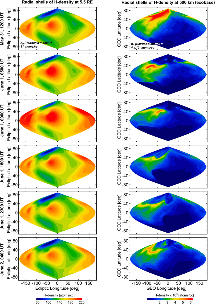
Figure 2. Temporal evolution of the exospheric H densities during the development of the storm. The first column displays radial shells of H-density at 5.5 $R_E$ geocentric distance in GSE coordinates. The second column shows H densities at the exobase (500 km altitude) obtained from the WACMM-X model in GEO coordinates. The H-density values estimated by Rairden’s model at these two distances are 81 and $4.4\times 10^4$ atoms/${\text{cm}}^3$, respectively.

During the geomagnetic storm, there was an evident global enhancement of H densities beyond 3 $R_E$ starting on May 31, $\sim$1800 UT, which lasted for almost 1 day until June 1, $\sim$1600 UT, followed by a slow recovery to quiet-time conditions. The radial shell in the third row of Figure 2 (left side) shows a total increase of exospheric $n_H$ of $\sim 22\%$ with respect to quiet-time densities. The increase is significantly higher in the dayside nose (including the dawn sector) and the nightside tail compared with other regions of the exosphere. It is noteworthy that exospheric H densities derived from TWINS/LAD instruments during these days are greater than those described by the (Rairden et al., 1986) model during both quiet- and storm-time, having a constant value of 81 atoms/${\text{cm}}^{-3}$. On the other hand, H density values in the exobase (right column) globally decrease during the storm with respect to quiet time conditions as a response to the increase in temperature.In this work, we use two exospheric models: the spherically symmetric and temporally static exosphere implemented by Rairden et al. (1986), hereafter referred to as the “static H” (StH) model, and the hybrid model derived from TWINS/LAD radiance data and WACCM-X predictions, referred to as the “dynamic H” (DynH) model. Figure 3 shows a numerical comparison between both models during the 1 June 2013 geomagnetic storm. Panel A shows the difference in H density distributions between both models expressed in a logarithmical scale for better visualization. Panel B shows the DynH/StH ratio as an alternative method to observe the variability of density distributions among the models.

Figure 3

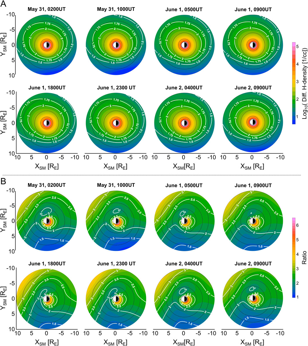
Figure 3. Quantitative comparison between exospheric models used in this study. (A) shows the difference in H densities between DynH and StH models expressed in ${\text{log}}_{10}$ scale through the development of the June 1 storm. Similarly, (B) shows global scale plots of the ratio DynH/StH. Black concentric and dashed circles in all plots indicate geocentric distances of 2, 4, 6, and 8 $R_E$.

Through the analysis of these plots, we found that the DynH model exhibits larger H densities than the StH model for all periods and at all altitudes (500 km–10 $R_E$). Although Figure 2 only shows the differences and ratios within the ${\text{XY}}_{SM}$ plane, we verified that H density is also greater at all latitudes. Panel A shows the density difference between models on a global scale. Since StH is fixed for all periods, an expansion of the DynH exosphere is evident (mostly in the dayside dawn sector) starting on 1 June 0500 UT, and lasting until 1 June 2300 UT. By the morning of June 2, the exospheric density distributions are similar to pre-storm conditions (e.g., see the contour line with level 1.75 at different time periods). Furthermore, panel B shows that within the ring current region in the equatorial plane (3–6 $R_E$), the DynH model provides densities $\sim$2 times greater than those from the StH model.

2.5 Ring current model: the comprehensive inner magnetosphere-ionosphere (CIMI) model

To determine the ring current development during the 1 June 2013 storm, we use the Comprehensive Inner Magnetosphere-Ionosphere (CIMI) model designed and implemented by Fok et al. (2014), Fok et al. (2021), which simulates the ring current ion fluxes and the magnetospheric electric field. CIMI is a kinetic model that calculates ion (0.1–500 keV) and electron (1 keV–6 MeV) distributions, the subauroral Region-2 field-aligned currents, the sub-auroral ionospheric potentials, and the plasmasphere distributions by solving (a) the bounce-averaged Boltzmann equation for the distribution functions of energetic ions and electrons, (b) the conservation equation of plasmasphere particles, and (c) the ionospheric current conservation equation for the ionospheric potential. The spatial domain of CIMI is circumscribed to the closed magnetic field region bounded by the dayside magnetopause located at a typical radial geocentric distance of 10 $R_E$. The model grid resolution is defined by 53 and 48 grid bins in magnetic latitude and local time of the ionospheric foot-points of the magnetic field lines, respectively. Current species supported by CIMI include ${\text{H}}^{+},{\text{O}}^{+},{\text{He}}^{+}$, and high-energy electrons. Also, CIMI accounts for several particle loss mechanisms such as (a) particle diffusion in energy and pitch angle due to interactions with plasma waves, (b) particle precipitation into the loss cone, and, of particular interest in this study, (c) charge exchange between ring current ions and exospheric neutral atoms. The charge exchange interaction is calculated in CIMI using the formula $-v{\sigma }_{sH}⟨n_H⟩f_s$ where $v$ is the ion velocity, ${\sigma }_{sH}$ is the energy-dependent charge exchange cross-section between ion species “s” and atomic hydrogen, and the terms $⟨n_H⟩$ and $f_s$ are the averaged H density and averaged ion distribution function along a given field line, respectively. Specific settings in the CIMI model used in this study are provided in the next section. The reader is referred to Fok et al. (2014), Fok et al. (2021) for further details of the CIMI model.

3 The role of the terrestrial exosphere in the ring current decay during the 1 June 2013 storm

3.1 Experiments’ settings

To assess the role of a realistic terrestrial exosphere in the ring current decay, we use the CIMI model to simulate the ring current ion fluxes and their dynamic response to two distinct exospheric models (StH and DynH) during 3 days from May 31 to 2 June 2013. Then, the CIMI model is configured to calculate the fluxes of ${\text{H}}^{+},{\text{O}}^{+}$, and high-energetic electrons (${\text{e}}^{-}$). We use the plasma sheet density and temperature from Tsyganenko et al. (2003) as the outer boundary condition, which is controlled by solar wind parameters. The ion composition of the plasma sheet is determined by the (Young et al., 1982; Pandya et al., 2018) formulations based on Kp, F10.7, and solar wind dynamic pressure (Psw). The ionospheric electric potential at the poleward boundary (71.4 deg) is specified by the Weimer 2K model (Weimer, 2001), and the electric field is calculated self-consistently within the CIMI domain (Fok et al., 2001). The magnetic field used is based on the TS04 model (Tsyganenko and Sitnov, 2005). Also, we only consider electron interactions with chorus waves, and besides the plasma loss to the magnetopause, charge exchange interactions with atomic H are the only ion loss mechanism included. Hence, we conducted two ring current simulations with these plasma parameters and magnetic field configuration, wherein only the exospheric H model was changed.

3.2 Impact of the geocorona on ring current dynamics

3.2.1 Temporal evolution of the ring current ion distribution

To examine the ring current development and its response to a given exospheric density model, we analyze the resulting ion fluxes for both “runs”. Figure 4 shows the ion flux comparison between CIMI simulations coupled with the static and dynamic H exospheric models during quiet time conditions, i.e., 31 May 0200 UT, and 1000 UT. For each species, the figure shows ion flux estimates using CIMI coupled with the StH and DynH models. To quantify the differences between runs, we calculated the log accuracy ratio, $\text{Log}(Q(r,\varphi ))$, where $Q(r,\varphi )$ is the ratio of the resulting ion flux using dynamic H to the resulting ion flux using static H at a given spatial location $(r,\varphi )$ in the equatorial plane, i.e., $Q(r,\varphi )=j_{\mathit{dynH}}(r,\varphi )/j_{\mathit{stH}}(r,\varphi )$ (Morley et al., 2018). Also, for a given period of time, the ion fluxes are provided in three energy ranges: 0.1–60 keV (low-energy), 60–121 keV (mid-energy), and 121–500 keV (high-energy). Note that each energy range has a distinct color bar scale (at the bottom of the Figure), which has been selected to highlight the differences in the ion fluxes for both simulations. With an identical format, Figures 5–7 depict the ion flux comparison during six additional periods within the peak of the storm as well as its recovery phase: 1 June 0500 UT/0900 UT, 1 June 1800 UT/2300 UT, and 2 June 0400 UT/0900 UT, respectively.

Figure 4

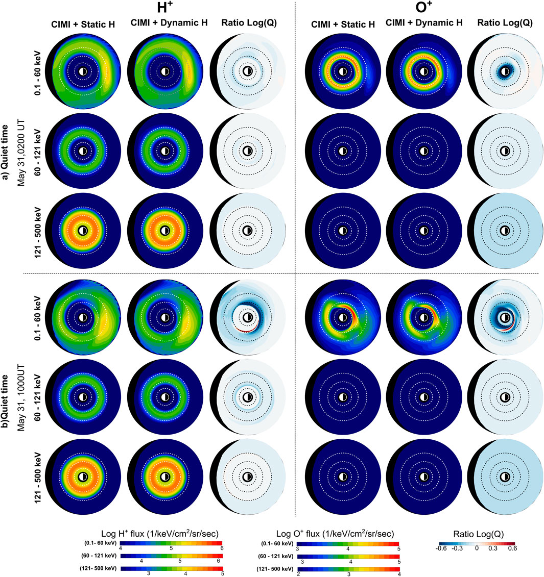
Figure 4. Comparison between ion fluxes generated by CIMI simulations using static and dynamic exospheric models for 31 May 0200 UT and 1000 UT. Each panel (out of 4) contains 9 graphs of equatorial ion flux distributions arranged as follows: the first and second columns depict ion flux results of using CIMI coupled with the static and dynamic H, respectively, and the third column shows the ion flux ratio defined as Log$(j_{\mathit{dynH}}/j_{\mathit{stH}})$. Rows from top to bottom show the ion flux results for three energy ranges: 0.1–60 keV (low-energy), 60–121 keV (mid-energy), and 121–500 keV (high-energy). The analysis has been done for both ion species in the simulations: ${\text{H}}^{+}$ and ${\text{O}}^{+}$. Also, the dashed curves indicate $L$-shells of 2, 4, and 6 $R_E$ (a, b) Quiet time.

Figure 5

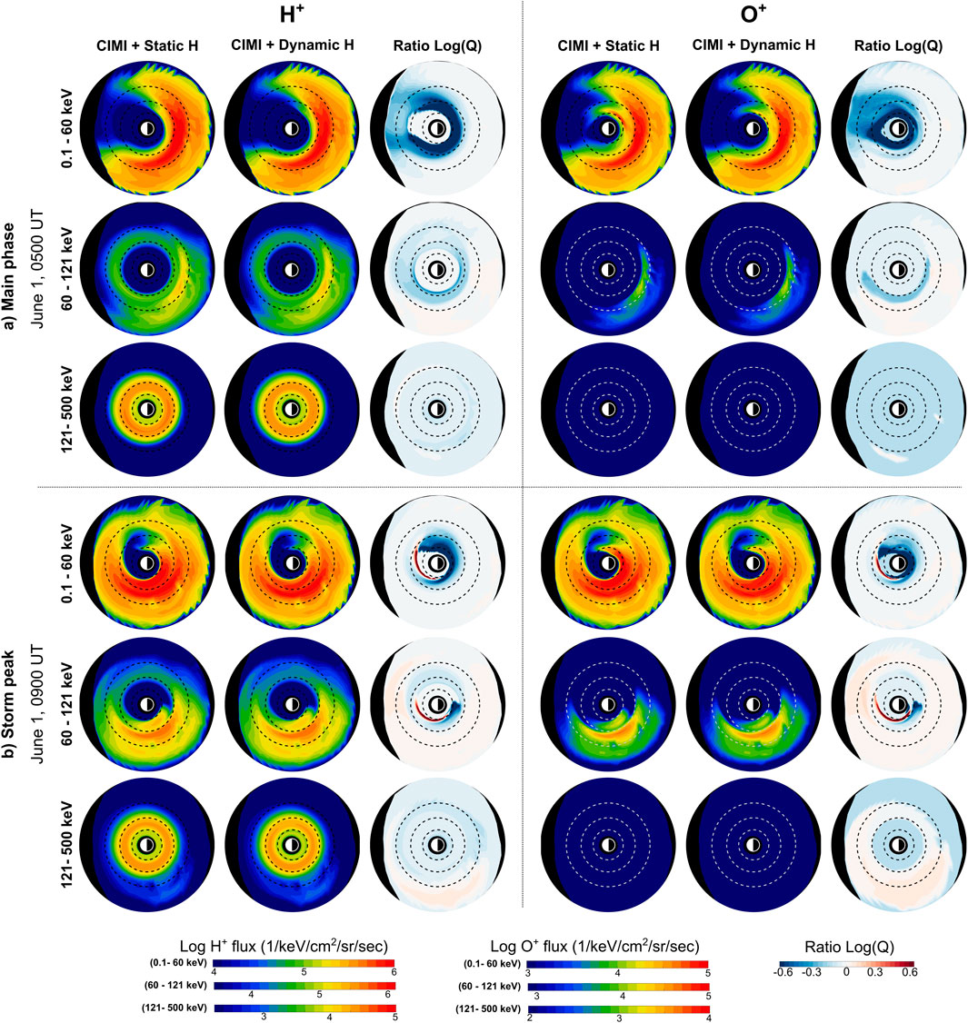
Figure 5. Comparison between ion fluxes generated by CIMI simulations using static and dynamic exospheric H models for 1 June 0500 UT and 1 June 0900 UT. This figure uses an identical format to Figure 4. (a) Main phase, (b) Storm peak.

Figure 6

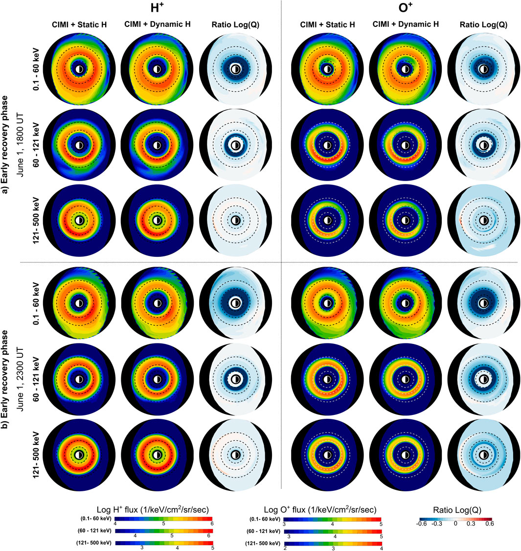
Figure 6. Comparison between ion fluxes generated by CIMI simulations using static and dynamic exospheric H models for 1 June 1800 UT and 1 June 2300 UT. This figure uses an identical format to Figure 4. (a) Early recovery phase (b) Early recovery phase.

Figure 7

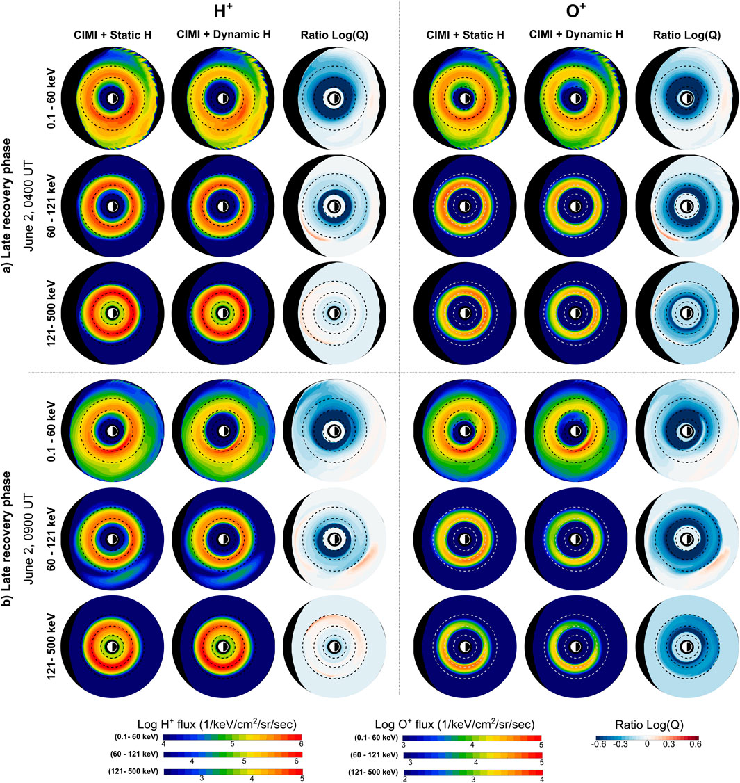
Figure 7. Comparison between ion fluxes generated by CIMI simulations using static and dynamic exospheric models for 2 June 0400 UT and 2 June 0900 UT. This figure uses an identical format to Figure 4. (a, b) Late recovery phase.

The Log$(Q)$ plots provide quantitative information regarding the regions where ion fluxes generated by the CIMI + DynH run are lower (depletion in blue color) or greater (enhancement in red color) with respect to those fluxes produced by the CIMI + StH configuration. The spatial (equatorial) distribution of these depletions or enhancements is highly correlated to.

• The exospheric H densities along a given field line, which, for the DynH model, are higher at all altitudes than those reported in the StH model (see Figure 3).

• The ion population along the field line, which depends on the pitch angle (PA) distribution and its consequently capacity to populate the low latitude/high altitude ring current regions (for a PA$\sim$ 90 deg) or the high latitude/low altitude zones (for PA $\sim 0/180$ deg);

• The ion energy, which defines the size of the charge exchange cross-section and, therefore, the efficiency of the ion-neutral interaction. Note that the cross-section for ${\text{H}}^{+}-$H significantly decreases as the proton energy increases while the cross-section for ${\text{O}}^{+}-$H does not vary much with ion energy (Fok et al., 1993).

• The self-consistent calculation of electric fields (within the ring current solution domain), which depends on the instantaneous ion population. Depending on their strength, electric fields may induce drifts of ions transporting them from one magnetic field line to another.

During the quiet time period (31 May 0200 UT in Figure 4), ratio plots with values of $\sim -0.1$ for ${\text{H}}^{+}$ at all energies indicate that charge exchange interaction with the dense DynH exospheric model has already reduced the ring current proton flux by a factor of $\sim 10\%$ (with respect to those calculated using StH). Although a similar behavior is expected in ratio plots for ${\text{O}}^{+}$, they show a strong depletion (Log$(Q)\sim -0.6$) at L shells $<$2 $R_E$ and at the lowest energy (0.1–60 keV). Pixel-wise data analysis revealed that ion fluxes in these regions are minimal, such that subtle variations due to charge exchange with H atoms produce these large ratios. For the sake of clarification, in this manuscript, we use the terms decrease or increase in flux to describe ion flux variations in the CIMI + DynH run with respect to the CIMI + StH run.

On 31 May 1000 UT, a depletion of low-energy proton fluxes (Log ($Q$)$\sim$-0.5) is observed in a narrow region at $L\sim 4$ in the midnight to dawn sector. For the same energy range, an increase in proton flux (Log ($Q$)$\sim$+0.5) is observed in a narrow band also near $L\sim 4$ in the dusk sector. Since Figure 2 demonstrated that DynH densities are larger than those from StH at all altitudes and periods, the increase of ion fluxes when DynH is used in the simulation is not expected to occur if we solely consider charge exchange processes. We identified that this feature is generated due to the effect of the electric field on the ring current ions. In these runs, the CIMI model calculates the electric field self-consistently, namely, the model accounts both for the effect of the electric field on the particles and for the feedback of the particles on the electric field. Thus, the electric field distributions in both runs are not identical, as they depend on the ion flux, which in turn varies via charge exchange with H atoms. A thorough analysis of the effect of the electric field over ion fluxes and the resulting variation of the ring current spatial structure has been reported in Ferradas et al. (2021). In our simulations (also including ${\text{O}}^{+}$ ions), this effect is displayed as a large enhancement (red) and/or depletions (blue) in very narrow regions close to the inner edges of the ring current. Also, this effect is most clearly seen in the distributions of the low-energy ions, it becomes less clear at the intermediate energies, and is not seen at the high energies. This is consistent with the fact that particles with increasing energy become more strongly controlled by magnetic drifts than by electric drifts.

In Section 4, we included equatorial plots of the electric field distributions for both runs to primarily depict the spatial differences produced by each model. It is noteworthy that the precise location of these enhancements or depletions due to electric fields requires a sophisticated analysis based on particle tracing for several hours [e.g., 4–6 h for 20 keV protons (Ferradas et al., 2021)], and its implementation is out of the scope of this study. Hence, the results shown in this and the following plots are the combined effect of charge exchange interactions and electric field variations, both being affected by the exospheric density.

During the main phase of the storm (1 June 0500 UT in Figure 5), there is a significant decrease in ion flux (Log ($Q$)$\sim \le -$0.6) for both species that occurs at the lowest energies (0.1$-$60 keV) in the region $L\in [\mathrm{2,4}]R_E$. In the case of mid-energies, the average ion flux, “calculated along the equatorial plane”, indicates a depletion for both species of less than $\sim 23\%$. The variation of high-energy proton fluxes is negligible $(<5\%)$ and expected due to the low cross-section ${\sigma }_{H^{+}H}$ for this energy range. On the other hand, the average depletion of high-energy ${\text{O}}^{+}$ flux is $\sim$14%.

During the storm peak (SYM-H index of −137 nT) on 1 June 0900 UT, the region with decreased flux for both species and for low energies became smaller and changed its location to lower altitudes. Also, an increase in the ion flux of $\sim 32\%$ in a narrow region is observed in the dayside sector for both ions in the low-to mid-energy range. This is highly associated with the continuous variations in the global electric field. In the case of high-energy ions, both species show slight depletions $(<20\%)$ and enhancements $(<15\%)$ of fluxes at low and high $L$ shells, respectively.

Figures 6, 7 show snapshots of ${\text{H}}^{+}$ and ${\text{O}}^{+}$ energy fluxes during the storm’s recovery phase when the ring current exhibits a more symmetric distribution in magnetic local time (MLT).

During 1 June 1800 UT and 2300 UT, low- and mid-energy ion fluxes for both species exhibit a significant decrease of $\sim$45% at $L\in [\mathrm{2,4}]R_E$ and for all MLTs. Additionally, a flux depletion of $\sim$15% is shown at L$\sim$6 $R_E$ near the pre-noon region. This feature is highly correlated to the one from the terrestrial exosphere, which also has higher H density in this sector at high geocentric distances (see Figures 2, 3). Moreover, the pre-noon sector corresponds to the reported MLT region where ions take longer to drift [e.g. (McIlwain, 1972; Kistler et al., 1989)] hence their distributions manifest stronger effects of charge exchange loss. These two facts explain the strong depletion of ion fluxes in this sector. In the case of high-energy fluxes for both species, they do not vary significantly during the storm’s recovery. Notably, high-energy ${\text{O}}^{+}$ fluxes exhibit higher depletion than the corresponding ${\text{H}}^{+}$ fluxes due to the large $O^{+}-H$ cross-section.

A similar trend occurs on 2 June 0400 UT and 0900 UT (see Figure 7); however, the low-energy flux depletion at L$\sim$6 $R_E$ and near the pre-noon region is increased up to $\sim 30\%$. This feature is correlated to a higher density of neutral H atoms during this period as a response to the storm. The red regions on these plots are associated with the temporal evolution of electric fields through the storm. Note that the ratio values are quite small (Log$(Q)\sim$+0.1) and occur in regions near the edges of the ring current where the ion fluxes are minimal.

3.2.2 Spatial variability of the ring current ion distribution in response to exospheric models

We independently analyze the differences in the radial and azimuthal domains to quantify the structural variation of equatorial ion fluxes resulting from using two distinct exospheric models in CIMI.

First, for each simulation, we calculated the MLT-integrated flux using the formula $J(\text{L},t)={\int }_0^{2\pi }j(\text{L},\varphi ,t)d\varphi$. Then, we calculated the ratio Log$(Q(\text{L},t))$ (with $Q(L,t)=J_{\mathit{dynH}}(\text{L},t)/J_{\mathit{stH}}(\text{L},t)$) for each time step and L-shell, as shown in Figure 8. Panels A, B, and C show the ratio Log$(Q(\text{L},t))$ calculated for ${\text{H}}^{+}$ ions for low-, mid-, and high-energy ranges, respectively. With a similar format, panels D, E, and F show Log$(Q(\text{L},t))$ values calculated for $O^{+}$ ions. In all cases, the yellow triangles and red diamonds indicate the L-shell location of the highest ion flux at a given time $t$ when exospheric models StH and DynH are used in CIMI, respectively. Also, the highest ion flux is plotted if and only if it is at least 25% greater than the mean of the fluxes in the full equatorial domain. The two bottom panels in Figure 8 are identical and show the Dst index for the storm to help the reader visualize the correlation between flux ratios and the phases of the storm.

Figure 8

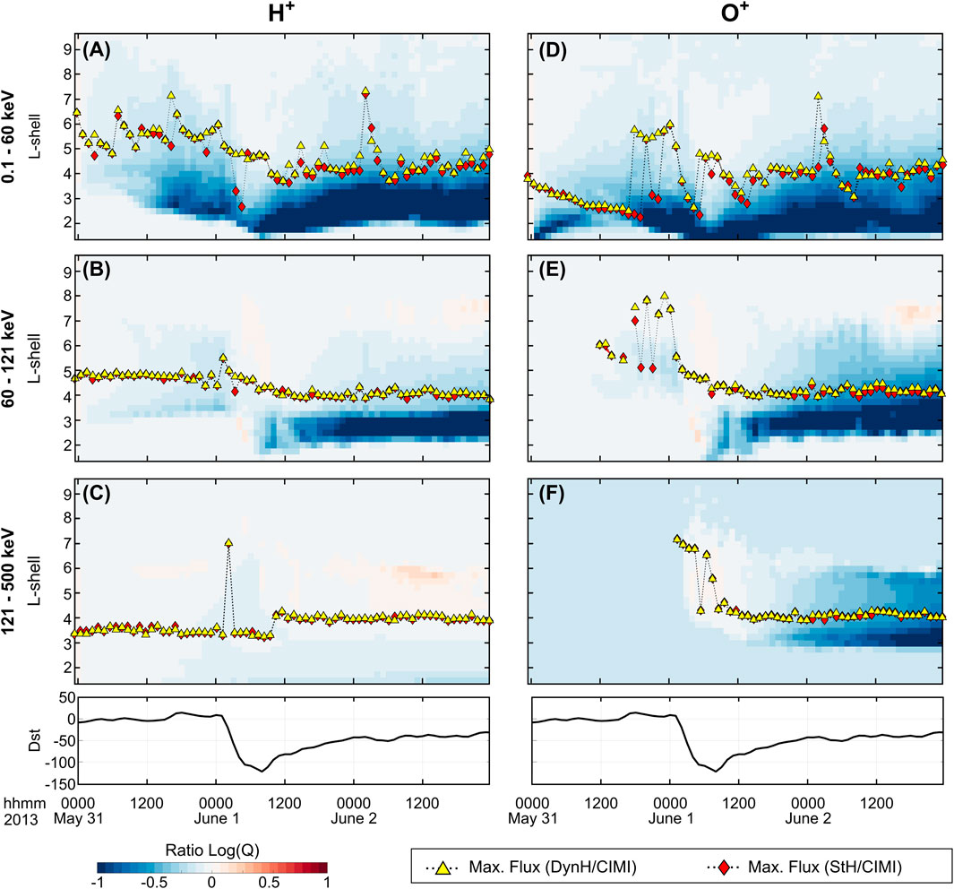
Figure 8. Comparison of MLT-integrated ion fluxes for both species. Panels (A-C) show MLT-integrated Log(Q) ratios corresponding to H+ for low-, mid-, and high-energy ranges, respectively. Panels (D-F) show Log(Q) ratios corresponfing to O+ for low-, mid-, and high-energy ranges. Yellow triangles indicate the L-shell of the ion flux peak in the equatorial solution domain of CIMI when the DynH model is used. Similarly, red diamonds indicate the ion flux peak in the simulation when the StH model is used. These plots serve to identify the L-shell location of ion flux variations during the development of the storm caused by using two distinct exospheric H models.

The higher H density distributions in the DynH model than in StH at ring current altitudes generate significant ion flux depletions during the storm’s development. Panels A and D show that for low-energy ${\text{H}}^{+}$ and ${\text{O}}^{+}$ fluxes, these depletions occur over a range of $L$-shells between 1.5 and 4 $R_E$ before and after the main phase of the storm, whereas during the storm main phase (1 June 0000UT to 1 June 0900UT), they occur confined to a much narrower $L$ range near the inner edge of the ring current. Also, the ratio Log$(Q)$ becomes intense during the recovery phase, which is in good agreement with the enhancement of atomic H during this period. Furthermore, we observe that the peaks of the ring current flux, when DynH is used (yellow triangles), are located at higher $L$-shells than those generated using StH (red diamonds). This trend demonstrates the role of exospheric H in determining the structure of the low-energy ring current.

The strong depletion of mid-energy ion fluxes starting after the storm peak (panels B and E) indicates that during the main phase, the injection of these ion energy populations to the ring current system is fast, and charge exchange effects are not strong. Thus, the differences between both runs are not significant. During the recovery phase, however, as activity decreases and ion transport to the inner magnetosphere takes longer, the effects of charge exchange interactions with neutral atoms become important, especially at $L$ shells 2 to 3 $R_E$. Panel C shows high-energy proton fluxes, which remain almost invariant to neutral populations (for either StH or DynH) since charge exchange becomes infrequent at this ion energy. On the other hand, panel F indicates that interaction between high-energy ${\text{O}}^{+}$ fluxes and exospheric H atoms is much more efficient than for protons (owing to the much larger charge exchange cross-section), producing significant depletions during the recovery phase at $L$ shells 3 to $\sim$6 $R_E$.

Second, we calculated the $L$ shell-integrated flux for each simulation using the formula $J(\varphi ,t)={\int }_{L_{\mathit{min}}}^{L_{\mathit{max}}}j(L,\varphi ,t)dL$, and also calculated the ratio Log$(Q(\varphi ,t))$ (with $Q=J_{\mathit{dynH}}(\varphi ,t)/J_{\mathit{stH}}(\varphi ,t)$) for each time step and MLT value, as shown in Figure 9. Panels A, B, and C show the ratio Log$(Q(\varphi ,t))$ calculated for ${\text{H}}^{+}$ ions for low-, mid-, and high-energy ranges, respectively. Similarly, panels E, F, and G show the Log$(Q(\varphi ,t))$ calculated for ${\text{O}}^{+}$ ions.

Figure 9

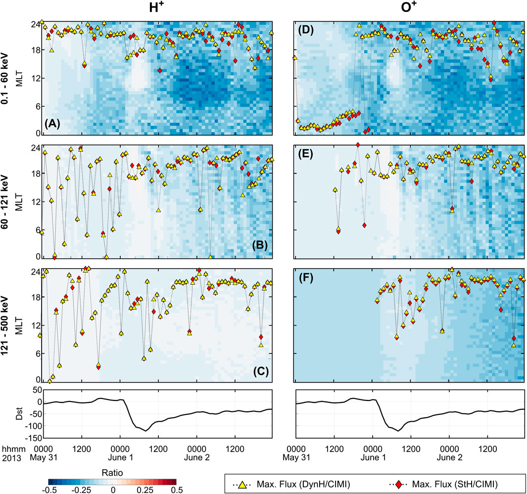
Figure 9. Comparison of L-shell integrated ion fluxes for both species. Panels (A-C) show the Log(Q) ratios corresponding to H+ for low-, mid-, and high-energy ranges, respectively. Panels (D-F) show the Log(Q) ratios corresponding to O+ for low-, mid-, and high-energy ranges, respectively. Yellow triangles and red diamonds follow identical format to Figure 8. These plots serve to identify the MLT (azimuthal) location of ion flux variations during the evolution of the storm yielded by the use of two exospheric H models.

Panels A and D in Figure 9 show that depletion in low-energy ion fluxes due to the use of the DynH model mainly occurs at the dayside region (MLT 6–18 h) during the recovery phase of the storm (1 June 1200 UT to 2 June 1200 UT). Note that ion depletion (both species) during the main phase of the storm (1 June 0000UT to 0900 UT) is almost negligible (Log ($Q$)$\sim$0) in the dusk region (MLT 12–18 h). This feature is not linked to the dynamic H distributions, which are always higher than StH densities at ring current altitudes, but to the ion density and its spatial distribution in the ring current system. In addition, we observe evident variation in the location of the ring current peak flux (red diamonds and yellow triangles) during the storm development, especially in the recovery phase. Panels B and E depict mid-energy ion flux depletions occurring more regularly along all MLT hours since, at these energies, the ring current ion distributions are more symmetric in MLT. Also, during the storm main phase, we found Log ($Q$)$\sim$0 since the fast ion drift during this period minimizes the effects of charge exchange losses. The temporal periodicity in Log$(Q)$ observed during the recovery phase is correlated to the ion rotation around the equatorial plane (Ferradas et al., 2021). On the other hand, panels C and F show the low dependence of high-energy ion fluxes on temporal variations in atomic H densities.

3.3 Impact of the geocorona on the total ring current energy

In this section, we calculated the temporal evolution of the total ring current energy (RCE) in units of [$10^{31}$eV] during the 1 June 2013 storm. The left panel in Figure 10 shows the total RCE from both runs using DynH (solid red line) and StH (dashed red line), along with the Dst index (dotted blue line) and its pressure-corrected version Dst* (dashed blue line). In general, the time-dependent structure of the total RCE from both runs exhibits good agreement with the trends in Dst*. Also, while the simulated ring current in both runs has nearly equal peak strength, the DynH run exhibits a faster recovery (after 1 June 0900UT), which is associated with the larger H densities in the DynH model at ring current altitudes and consequent stronger charge exchange loss during this period. To further quantify the relationship between RCEs, the ratio RCE-DynH/RCE-StH is calculated and displayed in the right panel of Figure 10. Before the storm onset, the total RCE in the DynH run is $\sim <5\%$ smaller than in the StH run. During the recovery phase, the total RCE in the DynH run constantly decays and becomes $\sim 32\%$ smaller than in the StH run on 2 June 2300UT. A simple analysis of the slope of the RCE-DynH/RCE-StH ratio during the recovery phase (after 1 June 0900UT) indicates that the “energy loss per day” in the ring current using the DynH model is $\sim 12.5\%$ faster than using the StH model.

Figure 10

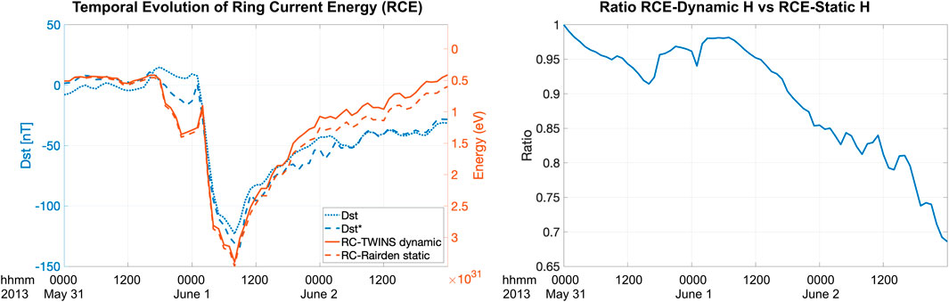
Figure 10. The left panel shows the measured Dst (dotted blue line) and Dst* (dashed blue line) indices and total simulated ring current energy for two runs conducted with the CIMI model. The right panel shows the ratio of total ring current energy using DynH and StH exospheric models.

3.4 Comparison of simulated ring current fluxes with in situ measurements from Van Allen Probes

Figure 11 compares simulated ring current proton fluxes (using DynH and StH) with in situ proton flux measurements acquired by the Helium, Oxygen, Proton, and Electron (HOPE) and the Radiation Belt Storm Probes Ion Composition Experiment (RBSPICE) mass spectrometers onboard NASA’s Van Allen Probes mission. Panels from top to bottom show (a) the proton (energy vs. time) flux spectrogram acquired by the HOPE + RBSPICE instruments during the period under study (May 31 to June 2) and covering ion energies from $1\times {10}^2$ to $5\times {10}^5$ eV, (b) the simulated proton flux spectrogram from the CIMI + StH run for the actual location of the Van Allen Probes A spacecraft, (c) the simulated proton flux for CIMI + DynH model for identical locations, (d) the ratio ${\text{Log}}_{10}(Q(E,t))$, where $Q=j_{\mathit{StH}}(E,t)/j_{\mathit{vap}}(E,t)$, and $E$ represents the energy channel, (e) the ratio ${\text{Log}}_{10}$($Q(E,\mathbf{r})$), where $Q=j_{\mathit{DynH}}(E,\mathbf{r})/j_{\mathit{vap}}(E,\mathbf{r})$, (f) the $L$ shell location of the Van Allen Probes A, and (g) the Sym-H index for the 1 June 2013 storm. With an identical format, Figure 12 shows oxygen ion spectrograms from CIMI simulations and in situ measurements from Van Allen Probes.

Figure 11

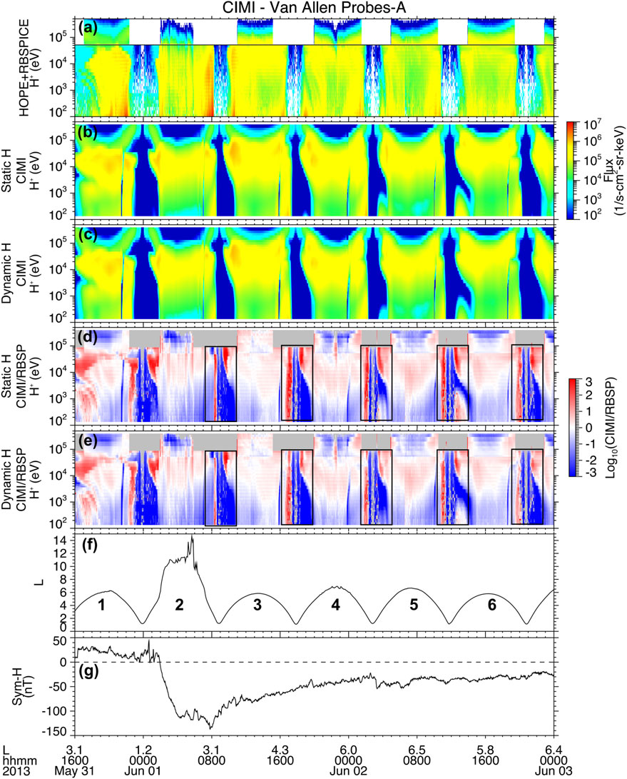
Figure 11. Comparison of proton energy spectrum simulated by CIMI with in situ measurements from HOPE + RBSPICE spectrographs onboard NASA’s Van Allen Probe mission. (a) shows the energy spectrum of in situ measurements provided by HOPE + RBSPICE (H + R) instruments, (b) shows the simulated spectrum from CIMI using the StH model, (c) shows the simulated spectrum from CIMI using the DynH model, (d) shows the ratio ${\text{Log}}_{10}$[Flux (CIMI + StH)/Flux (H + R)], (e) shows ${\text{Log}}_{10}$[Flux (CIMI + DynH)/Flux (H + R)], panel (f) shows the L-shell corresponding to the trajectory of Van Allen Probes spacecraft, and panel (g) shows the Sym-H index.

Figure 12

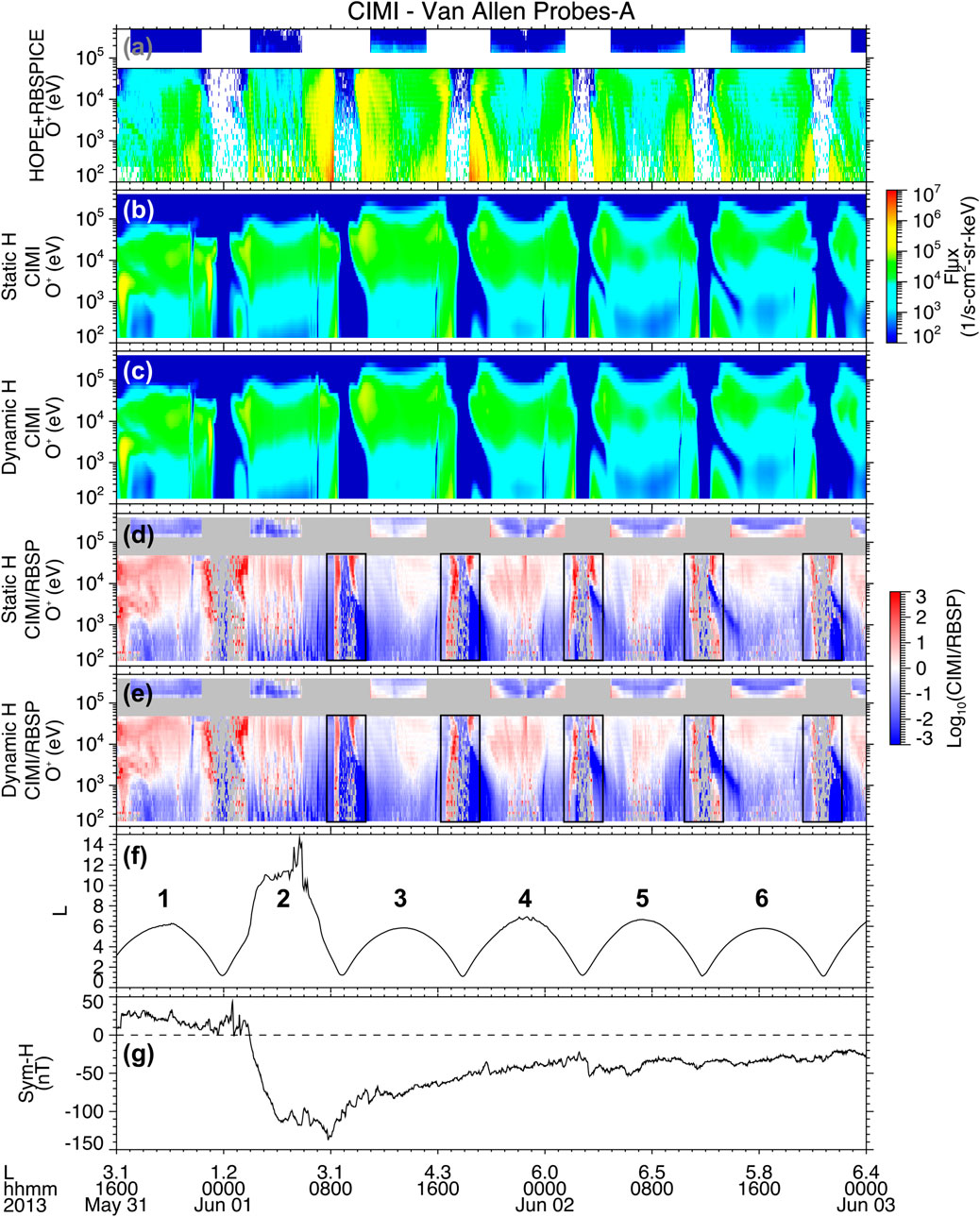
Figure 12. Comparison of O+ energy spectrum simulated by CIMI with in situ measurements from HOPE + RBSPICE spectrographs onboard NASA's Van Allen Probe mission. (a) shows the energy spectrum of in situ measurements provided by HOPE + RBSPICE (H + R) instruments, (b) shows the simulated spectrum from CIMI using the StH model, (c) shows the simulated spectrum from CIMI using the DynH model, (d) shows the ratio Log10[Flux (CIMI +StH)/Flux (H + R)], (e) shows Log10[Flux (CIMI + DynH)/Flux (H + R)], panel (f) shows the L-shell corresponding to the trajectory of Van Allen Probes spacecraft, and panel (g) shows the Sym-H index.

The analysis of CIMI + StH/RBSP (Figure 11d) and CIMI + DynH/RBSP (Figure 11e) ratios indicate that the simulated proton fluxes with both exospheric models have a reasonably good agreement with in situ observations (i.e., $|{\text{Log}}_{10}(Q)|<$ 1) when RBSP-A is located at $L\in [\mathrm{4,6.5}]R_E$. On the other hand, when the spacecraft is located at $L\sim <2R_E$, flux simulations with StH and DynH models exhibit a large ($|{\text{Log}}_{10}(Q)|>3$) to moderate ($|{\text{Log}}_{10}(Q)|\in [\mathrm{1,3}]$) over- and under-estimation at all energies. These features are similar in orbits 3, 4, 5, and 6 during the recovery phase of the storm and are highlighted with black line rectangles. The overestimation of proton fluxes at low $L$ near spacecraft perigee seems to be related to an undershielding effect in the CIMI model, which yields strong electric fields at low $L$ pushing ions, especially protons, deeper than observed. A simple comparison of the fluxes within the black line rectangles (panels e and d) indicates that using DynH slightly reduces the overestimation owing to its high H-density at ring current altitudes, e.g., on 02 June 0300 UT (between orbits 4 and 5), the ratio for proton fluxes, whose energy channel is $2\times 10^4$ eV, changes from ${\text{Log}}_{10}$(CIMI + StH/RBSP)$=+2.0$ to ${\text{Log}}_{10}$(CIMI + DynH/RBSP)$=+1.5$. A similar trend is found for ${\text{O}}^{+}$ ion fluxes, as shown in Figure 12. In this case, there is a lower overestimation of fluxes near the spacecraft perigee than those observed for protons as the undershielding effect in the CIMI model (mentioned above) is less efficient for heavy ions. Similar to the proton case, the use of DynH over the ${\text{O}}^{+}$ fluxes slightly reduces the overestimation near perigee, e.g., on 02 June 0300 UT (between orbits 4 and 5), the ratio for ${\text{O}}^{+}$ fluxes, whose energy channel is $2\times 10^4$ eV, changes from ${\text{Log}}_{10}$(CIMI + StH/RBSP)$=+2.5$ to ${\text{Log}}_{10}$(CIMI + DynH/RBSP)$=+2$.

Figure 13 shows the integrated ion energy flux (for both species) over the energy range of 0.1–500 keV along the path of RBSP-A during the 1 June 2013 storm. For comparison, we also calculated the integrated ion flux for CIMI + StH and CIMI + DynH simulations.

Figure 13

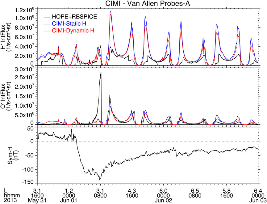
Figure 13. Comparison of integrated ion energy flux along the path of Van Allen Probes mission. The top panel shows the integrated proton energy flux for HOPE + RBSPICE instruments (black line), the CIMI + StH simulation (blue line), and the CIMI + DynH simulation (red line). With a similar format, the central panel shows the integrated ${\text{O}}^{+}$ energy flux. The bottom panel shows the Sym-H index during the 1 June 2013 storm.

The integrated proton energy flux obtained from CIMI simulations is significantly larger than those measured by RBSP-A at $L<5R_E$. This trend can be attributed to (1) the simulation settings, which only include limited ion loss processes since our goal in this study is to identify the impact of the exosphere in the ring current, and (2) an undershielding effect in the CIMI model, which allows ions deeper access than observed. With this in mind, we observe that using the DynH model in the simulations certainly reduces the integrated flux up to 25% compared to the results yielded by using StH (e.g., in the top panel on 01 June 1900 UT). The results for the ${\text{O}}^{+}$ integrated fluxes exhibit a better agreement with those obtained from CIMI simulations except near the storm’s peak. Similarly, the use of DynH in the ring current yields a reduction of integrated energy flux of up to $\sim 25\%$ with respect to the values obtained from simulations with StH model (e.g., in the middle panel on 02 June 1400 UT).

4 Discussions and conclusion

In this manuscript, we evaluated the role of a realistic exospheric model on the ring current dynamics during the geomagnetic storm that occurred on 1 June 2013. To do so, we used the CIMI model to simulate ring current ion fluxes that respond to two distinct exospheric models. The first is an empirical, temporally static and spherically symmetric model, StH, implemented by Rairden et al. (1986) using H Ly-$\alpha$ emission acquired by the DE1 mission. The second exospheric model, DynH, is an event-specific model derived from TWINS/LAD radiance data acquired from May 31 to 2 June 2013, to produce the exosphere beyond 3 $R_E$, which has been merged with a low-altitude, time-dependent exospheric density distribution obtained from the WACMM-X model. This hybrid model exhibits an asymmetric structure and shows significant H density variability during the storm development. We acknowledge that H-density values from altitudes between 500 km up to 2 $R_E$ of this model are not constrained by data or physics and have been extrapolated from their boundaries. This process has to be done due to the lack of Ly-$\alpha$ radiance data within this region during this storm. Then, we incorporated the two exospheric models in CIMI and simulated ring current proton and oxygen ion fluxes in the equatorial plane. The only ion loss process considered in the simulations, besides ion loss to the magnetopause, was charge exchange with exospheric H atoms.

In addition, the use of a self-consistent electric field in the CIMI model revealed how the inner magnetospheric electric field is indirectly affected by the exospheric density distributions. Specifically, electric fields are derived through the calculation of ionospheric conductivity and ring current pressure gradients. The latter directly depends on the ion flux, which varies due to the charge exchange with atomic H. Figure 14 shows the evolution of electric fields within the ring current region for simulations using the StH and DynH models. The periods correspond to those used in Figures 4–7. The third column shows the relative difference between electric fields calculated as $100\%\times$ (E (DynH)-E (StH))/(E (StH). These plots intend to show the reader that the electric fields vary (up to $\sim \pm$30%) in response to the exospheric model. However, the exact determination of how these electric fields affect the drift of ${\text{H}}^{+}$ and ${\text{O}}^{+}$ ions within the ring current domain requires the tracing of these particles for several hours, as shown by Ferradas et al. (2021). Such a process is out of the scope of our investigation.The conclusions from our study are the following:

1. Global exospheric density distributions derived from FUV observations during the 1 June 2013 storm are significantly asymmetric, with enhanced H densities along the Sun-Earth line (day and night side). Also, the exosphere is dynamic, and the global H densities increase in response to the evolution of the geomagnetic storm, which is associated with an increase in the temperature at the exobase (Chamberlain, 1963) and possible variations in the rate of charge exchange with plasmaspheric ions (Kuwabara et al., 2017).

2. H density values of a realistic exosphere (DynH) at 5.5$R_E$ and during quiet time are $\sim 35\%$ higher than those from the StH model, typically used in ring current simulations. Furthermore, this difference increases up to $\sim 50\%$ during storm time (See Figures 2, 3)

3. A general comparison of resulting proton fluxes during the whole storm period using the two exospheric models in CIMI reveals that the run with the DynH model reduces the fluxes up to $45\%$ for low-to-mid energy protons (0.1–121 keV) in comparison with those produced by the run using StH. The depletions for low-energy protons are predominantly localized at $L<4R_E$ during the main phase of the storm and the early recovery phase but extend up to $8R_E$ towards the dayside-dawn sector during the late recovery phase (after 2 June 0400 UT). Flux depletions for mid-energy protons are mostly stable within the region $L\in [\mathrm{2,6}]R_E$. On the other hand, high-energy protons do not show a significant response to the high H density of the DynH model, which is mainly associated with the small charge exchange cross-section for these proton energies (121–500 keV).

4. A similar trend is observed for low-to-mid energy ${\text{O}}^{+}$ fluxes during the storm development. Notwithstanding, high-energy ${\text{O}}^{+}$ ions respond to the H-density DynH model, showing up to $\sim 25\%$ stronger flux decay, especially in the late recovery phase, with respect to the results with the StH model (see Figures 5–7). Note that the ${\text{O}}^{+}-$H charge exchange cross-section decreases with energy, although much more gradually than the ${\text{H}}^{+}-$H cross-section, and it is at least 3 orders of magnitude greater than the ${\text{H}}^{+}-$H cross-section at high energies ($>$100 kev) (Ilie et al., 2013; Fok et al., 1993), which means that O+ have much shorter lifetimes at these energies and the effect of a denser exosphere is more notable.

5. Analysis of $L$-shell variations of “MLT-integrated” ring current ion fluxes (Figure 8) reveals that using the DynH exosphere reduces low-to-mid-energy proton and ${\text{O}}^{+}$ fluxes up to 60$\%$, in comparison with those produced by the StH model, particularly within $L$ shells 2 to 4 $R_E$ and during the storm’s recovery phase. See more details in Section 3.2.2.

6. Analysis of the azimuthal variations of “$L$-shell-integrated” ring current ion fluxes (Figure 9) shows that the DynH model yields $\sim 35\%$ (for ${\text{H}}^{+}$) and $\sim 25\%$ (for ${\text{O}}^{+}$) stronger depletions than the StH model at the dayside sector (MLT = 6–18 h). See more details in Section 3.2.2.

7. The use of the DynH model in the CIMI simulations slightly modifies the ring current flux structure, especially for low-energy ions. This is evidenced by the variations of the peak ion flux locations in Figures 8, 9, panels A and D (yellow triangles for DynH and red diamonds for StH).

8. In the late recovery phase, the total ring current energy using DynH is up to $\sim 32\%$ lower than that produced by the StH model. Also, the “energy loss per day” calculated for the run using DynH is $\sim 12.5\%$ faster than that obtained for the run that uses the StH model (See Figure 10).

9. Comparison of simulated ion fluxes with in situ measurements from HOPE/RBSPICE instruments onboard NASA’s Van Allen Probes mission indicates that CIMI systematically overestimates the ion fluxes at low $L$ shells $(<4R_E)$. Notwithstanding, the simulation using DynH provides fluxes 25% smaller than those obtained from the run with the StH model, thus improving the agreement with the measured values.

10. Using a self-consistent electric field in the simulations revealed that atomic H also had, to a lesser extent, an effect on the structure of the ring current. For example, in Figure 4, the ion flux maps for low energy ions on 31 May 10,000 UT, exhibit a narrow flux enhancement in the DynH run with respect to the StH (shown in red). This feature indicates that when the DynH model was used in CIMI, the inner boundary of the ring current slightly moved inward in the dusk region likely associated with an enhanced electric field along the ion drift trajectories. This analysis is with respect to the ring current structure derived from the StH model.

Figure 14

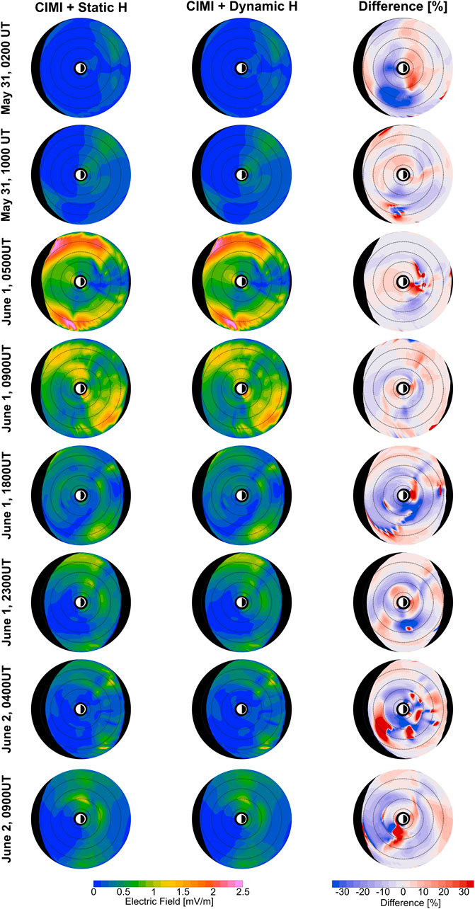
Figure 14. Temporal evolution of the electric field in the ring current for the two simulations. The right column shows the electric field difference between the two runs expressed in percentage values. Concentric black dashed circles indicate geocentric distances of 2, 4, 6 and 8 $R_E$

In summary, our study demonstrates that using a more realistic exospheric H density model reduces ring current ion flux via charge exchange interaction compared to historical H models. Also, an increase of ion fluxes is possible and mainly occurs near the edges of the ring current due to variability of the electric field, which in turn is linked to the neutral hydrogen population. Furthermore, our comparison study indicates that the depletion of ion fluxes is highly correlated to the three-dimensional structure of the exosphere, which clearly depends on the solar cycle and geomagnetic activity. It is noteworthy that each geomagnetic storm may have a particular effect on the exosphere as variations of exobase parameters will depend on the particle injection on the poles, the location of the poles (season), and solar FUV emission.

We acknowledge that our study does not include any interaction of the exosphere and ring current with the terrestrial plasmasphere, which is highly dynamic during storm time. Through charge exchange, plasmaspheric ions can heat atomic H, allowing neutral particles to suddenly populate higher altitudes or even enforce escape (Kuwabara et al., 2017; Bishop and Chamberlain, 1987). Such an effect is not considered in the extrapolation of H densities from the exobase to the optically thin region. On the other hand, the production of plasmaspheric ions (e.g., protons), in turn, depends on low-altitude exospheric and thermospheric H atoms that charge exchange with topside ionospheric ${\text{O}}^{+}$ (Krall et al., 2018; Kotov et al., 2023). Furthermore, the interaction between ring current ions and exospheric H atoms also produces cold ions that refill the plasmasphere during geomagnetic storms (Liu et al., 2022). Hence, future work in this area may include investigating these different mechanisms as a complete ring current-plasmasphere - exosphere system using modeling tools as well as available remote sensing observations of ENAs, and Lyman-Alpha (121.6 nm) and EUV (30.8 nm) emissions.

Finally, this study aims to communicate to the magnetospheric community the importance of the terrestrial exosphere in magnetospheric simulations and the opportunity to use actual data from NASA’s Carruthers Geocoronal Observatory (to be launched in 2025), which will image the exosphere in Ly-$\alpha$ and consequently provide time-dependent, global H density distributions from the thermosphere to several tens of Earth radii.

Data availability statement

NASA's TWINS LAD radiance data is publicly available at the Space Physics Data Facility (https://spdf.gsfc.nasa.gov/). Solar Lyman-Alpha irradiance needed for tomographic reconstructions of exospheric densities is publicly available at LISIRD/LASP repository (https://lasp.colorado.edu/lisird/). The HOPE particle data are available from the Van Allen Probes ECT website at https://rbsp-ect.newmexicoconsortium.org/science/DataDirectories.php. Thermospheric temperature and density were obtained from the WACCM-X model through the Comunity Coordinated Modeling Center (CCMC) and the run (Gonzalo_CuchoPadin_091123_IT_1) is publicly available at https://ccmc.gsfc.nasa.gov.

Author contributions

GC-P: Conceptualization, Formal Analysis, Investigation, Methodology, Writing–original draft, Writing–review and editing. CF: Conceptualization, Formal Analysis, Funding acquisition, Investigation, Methodology, Project administration, Writing–review and editing. M-CF: Conceptualization, Formal Analysis, Methodology, Writing–review and editing. LW: Writing–review and editing. JZ: Data curation, Writing–review and editing. S-BK: Formal Analysis, Methodology, Writing–review and editing.

Funding

The author(s) declare that financial support was received for the research, authorship, and/or publication of this article. The author(s) declare that financial support was received for the research, authorship, and/or publication of this article. This research was supported by the NSF-GEM award 2225363 and the NASA Goddard Space Flight Center through Cooperative Agreement 80NSSC21M0180 to Catholic University, Partnership for Heliophysics and Space Environment Research (PHaSER).

Acknowledgments

The authors thank the TWINS team (PI Dave McComas) for making this work possible. The authors also acknowledge the International Space Science Institute on the ISSI team titled “The Earth’s Exosphere and its Response to Space Weather.”

Conflict of interest

The authors declare that the research was conducted in the absence of any commercial or financial relationships that could be construed as a potential conflict of interest.

Generative AI statement

The author(s) declare that no Generative AI was used in the creation of this manuscript.

Publisher’s note

All claims expressed in this article are solely those of the authors and do not necessarily represent those of their affiliated organizations, or those of the publisher, the editors and the reviewers. Any product that may be evaluated in this article, or claim that may be made by its manufacturer, is not guaranteed or endorsed by the publisher.

References

Bailey, J., and Gruntman, M. (2011). Experimental study of exospheric hydrogen atom distributions by Lyman-alpha detectors on the TWINS mission. J. Geophys. Res. Space Phys. 116, 1–9. doi:10.1029/.2011JA016531

CrossRef Full Text | Google Scholar

Baliukin, I. I., Bertaux, J.-L., Quémerais, E., Izmodenov, V. V., and Schmidt, W. (2019). SWAN/SOHO Lyman-alpha mapping: the hydrogen geocorona extends well beyond the Moon. J. Geophys. Res. Space Phys. 124, 861–885. doi:10.1029/2018JA026136

CrossRef Full Text | Google Scholar

Beth, A., Garnier, P., Toublanc, D., Dandouras, I., and Mazelle, C. (2016). Theory for planetary exospheres: I. Radiation pressure effect on dynamical trajectories. Icarus 266, 410–422. doi:10.1016/j.icarus.2015.10.018

CrossRef Full Text | Google Scholar

Beth, A., Garnier, P., Toublanc, D., Dandouras, I., Mazelle, C., and Kotova, A. (2014). Modeling the satellite particle population in the planetary exospheres: application to Earth, Titan and Mars. Icarus 227, 21–36. doi:10.1016/j.icarus.2013.07.031

CrossRef Full Text | Google Scholar

Bishop, J., and Chamberlain, J. W. (1987). Geocoronal structure: 2. inclusion of a magnetic dipolar plasmasphere. J. Geophys. Res. Space Phys. 92, 12377–12388. doi:10.1029/JA092iA11p12377

CrossRef Full Text | Google Scholar

Brandt, J. C., and Chamberlain, J. W. (1959). Interplanetary gas. I. Hydrogen radiation in the night sky. Astrophys. J. 130, 670–682. doi:10.1086/146756

CrossRef Full Text | Google Scholar

Chamberlain, J. W. (1963). Planetary coronae and atmospheric evaporation. Planet. Space Sci. 11, 901–960. doi:10.1016/0032-0633(63)90122-3

CrossRef Full Text | Google Scholar

Cucho-Padin, G., Connor, H., Jung, J., Shoemaker, M., Murphy, K., Sibeck, D., et al. (2024). A feasibility study of 4-d tomography of soft x-ray magnetosheath emissivities using multi-spacecraft measurements. Front. Astronomy Space Sci. 11. doi:10.3389/fspas.2024.1379321

CrossRef Full Text | Google Scholar

Cucho-Padin, G., Kameda, S., and Sibeck, D. G. (2022). The earth’s outer exospheric density distributions derived from procyon/laica uv observations. J. Geophys. Res. Space Phys. 127, e2021JA030211. doi:10.1029/2021JA03021110.1029/2021ja030211E2021JA030211.2021JA030211

CrossRef Full Text | Google Scholar

Cucho-Padin, G., and Waldrop, L. (2018). Tomographic estimation of exospheric hydrogen density distributions. J. Geophys. Res. Space Phys. 123, 5119–5139. doi:10.1029/2018ja025323

CrossRef Full Text | Google Scholar

Cucho-Padin, G., and Waldrop, L. (2019). Time-dependent response of the terrestrial exosphere to a geomagnetic storm. Geophys. Res. Lett. 46, 11661–11670. doi:10.1029/2019gl084327

CrossRef Full Text | Google Scholar

Dessler, A. J., and Parker, E. N. (1959). Hydromagnetic theory of geomagnetic storms. J. Geophys. Res. (1896-1977) 64, 2239–2252. doi:10.1029/JZ064i012p02239

CrossRef Full Text | Google Scholar

Emmert, J. T., Drob, D. P., Picone, J. M., Siskind, D. E., Jones, Jr. M., Mlynczak, M. G., et al. (2021). NRLMSIS 2.0: a whole-atmosphere empirical model of temperature and neutral species densities. Earth Space Sci. 8, e2020EA001321. doi:10.1029/2020ea001321

CrossRef Full Text | Google Scholar

Ferradas, C., Reeves, G., Larsen, B., Skoug, R., Zhang, J.-C., Funsten, H., et al. (2021). The effects of the location and the timing of local convection electric field enhancements in the formation of ion multiple-nose structures. J. Atmos. Solar-Terrestrial Phys. 216, 105534. doi:10.1016/j.jastp.2020.105534

CrossRef Full Text | Google Scholar

Ferradas, C. P., Zhang, J.-C., Kistler, L. M., and Spence, H. E. (2015). Heavy-ion dominance near cluster perigees. J. Geophys. Res. Space Phys. 120, 10,485–510. doi:10.1002/2015JA021063

CrossRef Full Text | Google Scholar

Ferradas, C. P., Zhang, J.-C., Spence, H. E., Kistler, L. M., Larsen, B. A., Reeves, G., et al. (2016). Ion nose spectral structures observed by the van allen probes. J. Geophys. Res. Space Phys. 121 (12). doi:10.1002/2016JA022942

CrossRef Full Text | Google Scholar

Fok, M.-C., Buzulukova, N. Y., Chen, S.-H., Glocer, A., Nagai, T., Valek, P., et al. (2014). The comprehensive inner magnetosphere-ionosphere model. J. Geophys. Res. Space Phys. 119, 7522–7540. doi:10.1002/2014ja020239

CrossRef Full Text | Google Scholar

Fok, M.-C., Kang, S.-B., Ferradas, C. P., Buzulukova, N. Y., Glocer, A., and Komar, C. M. (2021). New developments in the comprehensive inner magnetosphere-ionosphere model. J. Geophys. Res. Space Phys. 126, e2020JA028987. doi:10.1029/2020ja028987

CrossRef Full Text | Google Scholar

Fok, M. C., Kozyra, J. U., Nagy, A. F., Rasmussen, C. E., and Khazanov, G. V. (1993). Decay of equatorial ring current ions and associated aeronomical consequences. J. Geophys. Res. Space Phys. 98, 19381–19393. doi:10.1029/93JA01848

CrossRef Full Text | Google Scholar

Fok, M.-C., Wolf, R. A., Spiro, R. W., and Moore, T. E. (2001). Comprehensive computational model of earth’s ring current. J. Geophys. Res. Space Phys. 106, 8417–8424. doi:10.1029/2000JA000235

CrossRef Full Text | Google Scholar

Hodges, R. R. (1994). Monte Carlo simulation of the terrestrial hydrogen exosphere. J. Geophys. Res. Space Phys. 99, 23229–23247. doi:10.1029/.94JA02183

CrossRef Full Text | Google Scholar

Ilie, R., Liemohn, M. W., Toth, G., and Skoug, R. M. (2012). Kinetic model of the inner magnetosphere with arbitrary magnetic field. J. Geophys. Res. Space Phys. 117. doi:10.1029/2011ja017189

CrossRef Full Text | Google Scholar

Ilie, R., Skoug, R., Funsten, H. O., Liemohn, M. W., Bailey, J. J., and Gruntman, M. (2013). The impact of geocoronal density on ring current development. J. Atmos. Solar-Terrestrial Phys. 99, 92–103. doi:10.1016/j.jastp.2012.03.010

CrossRef Full Text | Google Scholar

Jordanova, V. K. (2020). “Chapter 6 - ring current decay,” in Ring current investigations. Editors V. K. Jordanova, R. Ilie, and M. W. Chen (Elsevier), 181–223. doi:10.1016/B978-0-12-815571-4.00006-8

CrossRef Full Text | Google Scholar

Kistler, L. M., Ipavich, F. M., Hamilton, D. C., Gloeckler, G., Wilken, B., Kremser, G., et al. (1989). Energy spectra of the major ion species in the ring current during geomagnetic storms. J. Geophys. Res. Space Phys. 94, 3579–3599. doi:10.1029/JA094iA04p03579

CrossRef Full Text | Google Scholar

Kistler, L. M., Möbius, E., Klumpar, D. M., Popecki, M. A., Tang, L., Jordanova, V., et al. (1998). Fast/teams observations of charge exchange signatures in ions mirroring at low altitudes. Geophys. Res. Lett. 25, 2085–2088. doi:10.1029/98GL00331

CrossRef Full Text | Google Scholar

Kotov, D., Richards, P. G., Reznychenko, M., Bogomaz, O., Truhlík, V., Nossal, S., et al. (2023). Interhemispheric ionosphere-plasmasphere system shows a high sensitivity to the exospheric neutral hydrogen density: a caution of the global reference atmospheric model hydrogen density. Front. Astronomy Space Sci. 10. doi:10.3389/.fspas.2023.1113706

CrossRef Full Text | Google Scholar

Krall, J., Glocer, A., Fok, M.-C., Nossal, S. M., and Huba, J. D. (2018). The unknown hydrogen exosphere: space weather implications. Space weather. 16, 205–215. doi:10.1002/2017SW001780

CrossRef Full Text | Google Scholar

Kuwabara, M., Yoshioka, K., Murakami, G., Tsuchiya, F., Kimura, T., Yamazaki, A., et al. (2017). The geocoronal responses to the geomagnetic disturbances. J. Geophys. Res. Space Phys. 122, 1269–1276. doi:10.1002/2016ja023247

CrossRef Full Text | Google Scholar

Liu, J., Ilie, R., Borovsky, J. E., and Liemohn, M. W. (2022). A new mechanism for early-time plasmaspheric refilling: the role of charge exchange reactions in the transport of energy and mass throughout the ring current—plasmasphere system. J. Geophys. Res. Space Phys. 127, e2022JA030619. doi:10.1029/2022ja030619

PubMed Abstract | CrossRef Full Text | Google Scholar

Lundin, R., Lyons, L. R., and Pissarenko, N. (1980). Observations of the ring current composition at l 4. Geophys. Res. Lett. 7, 425–428. doi:10.1029/GL007i006p00425

CrossRef Full Text | Google Scholar

McComas, D. J., Allegrini, F., Baldonado, J., Blake, B., Brandt, P. C., Burch, J., et al. (2009). The two wide-angle imaging neutral-atom spectrometers (TWINS) NASA mission-of-opportunity. Space Sci. Rev. 142, 157–231. doi:10.1007/s11214-008-9467-4

CrossRef Full Text | Google Scholar

McIlwain, C. E. (1972). “Plasma convection in the vicinity of the geosynchronous orbit,” in Earth’s magnetospheric processes. Editor B. M. McCormac (Dordrecht: Springer Netherlands), 268–279.

CrossRef Full Text | Google Scholar

Moldwin, M. B., Downward, L., Rassoul, H. K., Amin, R., and Anderson, R. R. (2002). A new model of the location of the plasmapause: crres results. J. Geophys. Res. Space Phys. 107 (SMP 2–1), 2–9. doi:10.1029/2001JA009211

CrossRef Full Text | Google Scholar

Morley, S. K., Brito, T. V., and Welling, D. T. (2018). Measures of model performance based on the log accuracy ratio. Space weather. 16, 69–88. doi:10.1002/.2017SW001669

CrossRef Full Text | Google Scholar

Nossal, S. M., Mierkiewicz, E. J., and Roesler, F. L. (2012). Observed and modeled solar cycle variation in geocoronal hydrogen using NRLMSISE-00 thermosphere conditions and the bishop analytic exosphere model. J. Geophys. Res. Space Phys. 117. doi:10.1029/2011ja017074

CrossRef Full Text | Google Scholar

Pandya, M., Veenadhari, B., Nosé, M., Kumar, S., Reeves, G. D., and Lui, A. T. Y. (2018). Characteristics of storm time ion composition in the near-earth plasma sheet using geotail and rbsp measurements. Earth, Planets Space 70, 203. doi:10.1186/s40623-018-0977-3

CrossRef Full Text | Google Scholar

Qin, J., Waldrop, L., and Makela, J. J. (2017). Redistribution of H atoms in the upper atmosphere during geomagnetic storms. J. Geophys. Res. Space Phys. 122, 10,686–710. doi:10.1002/2017ja024489

CrossRef Full Text | Google Scholar

Rairden, R. L., Frank, L. A., and Craven, J. D. (1986). Geocoronal imaging with dynamics explorer. J. Geophys. Res. Space Phys. 91, 13613–13630. doi:10.1029/ja091ia12p13613

CrossRef Full Text | Google Scholar

Tsyganenko, N. A., Singer, H. J., and Kasper, J. C. (2003). Storm-time distortion of the inner magnetosphere: how severe can it get? J. Geophys. Res. Space Phys. 108. doi:10.1029/2002ja009808

CrossRef Full Text | Google Scholar

Tsyganenko, N. A., and Sitnov, M. I. (2005). Modeling the dynamics of the inner magnetosphere during strong geomagnetic storms. J. Geophys. Res. Space Phys. 110. doi:10.1029/2004JA010798

CrossRef Full Text | Google Scholar

Waldrop, L., and Paxton, L. J. (2013). Lyman-alpha airglow emission: implications for atomic hydrogen geocorona variability with solar cycle. J. Geophys. Res. Space Phys. 118, 5874–5890. doi:10.1002/jgra.50496

CrossRef Full Text | Google Scholar

Weimer, D. R. (2001). An improved model of ionospheric electric potentials including substorm perturbations and application to the geospace environment modeling november 24, 1996, event. J. Geophys. Res. Space Phys. 106, 407–416. doi:10.1029/2000ja000604

CrossRef Full Text | Google Scholar

Young, D. T., Balsiger, H., and Geiss, J. (1982). Correlations of magnetospheric ion composition with geomagnetic and solar activity. J. Geophys. Res. Space Phys. 87, 9077–9096. doi:10.1029/ja087ia11p09077

CrossRef Full Text | Google Scholar

Zesta, E., and Oliveira, D. M. (2019). Thermospheric heating and cooling times during geomagnetic storms, including extreme events. Geophys. Res. Lett. 46, 12739–12746. doi:10.1029/2019GL085120

CrossRef Full Text | Google Scholar

Zoennchen, J., Cucho-Padin, G., Waldrop, L., and Fahr, H. (2024). Comparison of terrestrial exospheric hydrogen 3d distributions at solar minimum and maximum using twins lyman-alpha observations. Front. Astronomy Space Sci. 11. doi:10.3389/fspas.2024.1409744

CrossRef Full Text | Google Scholar

Zoennchen, J. H., Nass, U., and Fahr, H. J. (2013). Exospheric hydrogen density distributions for equinox and summer solstice observed with TWINS1/2 during solar minimum. Ann. Geophys. 31, 513–527. doi:10.5194/angeo-31-513-2013

CrossRef Full Text | Google Scholar

Zoennchen, J. H., Nass, U., and Fahr, H. J. (2015). Terrestrial exospheric hydrogen density distributions under solar minimum and solar maximum conditions observed by the TWINS stereo mission. Ann. Geophys. 33, 413–426. doi:10.5194/angeo-33-413-2015

CrossRef Full Text | Google Scholar

Zoennchen, J. H., Nass, U., Fahr, H. J., and Goldstein, J. (2017). The response of the H geocorona between 3 and 8 R_e to geomagnetic disturbances studied using TWINS stereo Lyman-α data. Ann. Geophys. 35, 171–179. doi:10.5194/angeo-35-171-2017

CrossRef Full Text | Google Scholar