Application of a conditional generative adversarial network to denoising solar observations

The Extreme Ultraviolet Imaging Spectrometer (EIS) on the Hinode spacecraft has substantially advanced our understanding of the Sun’s upper atmosphere. Unfortunately, after being in operation since 2006, the EIS detectors have become noisy, which poses a challenge to data analysis. This paper presents a Conditional Generative Adversarial Network (cGAN) tailored to address the unique noise characteristics inherent in EIS data over the mission. Generative Adversarial Networks are deep learning models that learn to generate realistic data by training a pair of networks in an adversarial process, a mechanism that makes them particularly effective at capturing complex data distributions. Our cGAN model employs a U-Net-based generator and a conditioned discriminator, and it is trained and validated on a synthetic dataset designed to simulate the noise characteristics of EIS observations. The model converges quickly and produces denoised images that closely resemble the ground truth. Application to real EIS observations produces encouraging results, with the model effectively removing noise and largely preserving the spatial and spectral features of the data. When comparing the results of Gaussian fits to the line profiles, however, we find that the model produces only a modest enhancement over the current interpolation method.

1 Introduction

Spectrally resolved observations of the solar atmosphere provide many important clues to understanding the physical processes that drive the Sun’s dynamic behavior. The Extreme Ultraviolet Imaging Spectrometer (EIS) aboard the Hinode spacecraft was developed to provide spectrally resolved observations of the solar atmosphere in the extreme ultraviolet (EUV) wavelength range (Culhane et al., 2007). Launched in 2006, EIS has been providing detailed measurements of the solar corona for more than 17 years and has made many important discoveries (e.g., Al-Janabi et al., 2019).

Over the course of the Hinode mission the EIS detectors have developed numerous “warm pixels” (e.g., BenMoussa et al., 2013). These warm pixels are characterized by a high dark current that accumulates along with the solar signal during an observation. The warm pixels are likely caused by a combination of exposure to radiation on orbit and a thermal design that does not allow the detectors to be cooled optimally. The warm pixels are randomly distributed. Their number has increased over the mission, but appears to have plateaued at approximately 30% of the detector area.

The current approach to dealing with the warm pixels is interpolation^{1, 2, 3}. Warm pixel maps are created by thresholding dark images taken with the shutter closed and then interpolating values at these locations in the observations. Because the spectral features EIS observes are generally Gaussian, it is still possible to infer the moments of the line profiles, at least for the strongest emission lines. The weaker lines, however, are significantly affected by the noise from residual warm pixels even after interpolation. The purpose of this paper is to explore the use of machine learning to improve the quality of EIS data by removing the effects of the warm pixels.

Over the years, the challenge of image denoising has given rise to a plethora of techniques (Gupta and Gupta, 2013; Motwani et al., 2004; Fan et al., 2019; Tian et al., 2020a), underscoring the complexity and importance of the problem. The field has investigated diverse filtering methods (Mallat and Hwang, 1992; Donoho, 1995; Fodor and Kamath, 2003; Coifman and Donoho, 1995; Yang et al., 1995), various statistical approaches (Lang et al., 1995; Bui and Chen, 1998; Baraniuk, 1999), and multiple feed-forward machine learning strategies (Zhang et al., 2017; Tian et al., 2020b), each achieving significant outcomes in its respective domain.

The noise patterns in EIS images are distinctive, and the level of noise is significantly higher than in other comparable data sources. Such complexities often result in the suboptimal performance of the models previously mentioned. Recognizing this, we chose to develop a Conditional Generative Adversarial Network (cGAN), drawing inspiration from Isola et al.‘s foundational work on image-to-image translation (Isola et al., 2017). GANs are deep learning systems that pit two neural networks against each other — a generator that creates data and a discriminator that evaluates it — resulting in the production of increasingly realistic synthetic content. GANs have been successfully applied to a wide range of problems, including generating photorealistic faces, converting sketches to images, and enhancing low-resolution images.

GANs have consistently demonstrated superiority over traditional methods in modeling complex data distributions and producing realistic outputs (Goodfellow et al., 2020; Creswell et al., 2018; Zahin et al., 2021). Their capacity to emulate the underlying complexities within data distributions renders them as prime candidates for denoising applications. A cGAN, with its ability to utilize conditional inputs, promises a more focused and potent approach, capitalizing on additional information during training — in our context, the noisy EIS images.

Utilizing GANs for denoising is a well-established strategy, as shown by Li et al. (2021) in medical image denoising. Its potential as a robust denoising tool is further supported by several studies in diverse scenarios (Yin et al., 2021; Li et al., 2020; Chen et al., 2020).

Within the ever-evolving landscape of GANs, certain architectures, namely, DiscoGAN (Kim et al., 2017), StyleGAN (Abdal et al., 2019), and PC-WGAN (Cao et al., 2018), exhibit heightened complexity. Though these architectures are undeniably powerful and capable of producing images ex nihilo, their application to our specific challenge could be deemed disproportionate. Given the inherent characteristics of EIS images and the absence of prominent macro structures, a comprehensive reconstruction of images is not just formidable, but also potentially superfluous. Our primary objective is to enhance the extant data by methodically removing noise, and for this nuanced task, our selected cGAN model appears to be the best approach.

2 The EIS instrument

The EIS instrument on Hinode provides spectroscopic observations in two spectral ranges, 171–212 Å and 245–291 Å, with a spectral resolution of about 22 mÅ and a spatial sampling of $1^{\prime \prime }$ along the slit. The point spread function for EIS is approximately $3^{\prime \prime }$ FWHM⁴ (see also Brooks et al., 2012). Solar images can be made by stepping the slit over a region of the Sun and taking an exposure at each position. Relatively strong emission lines from Fe VIII–Fe XVI and Ca XIV–Ca XVII allow for excellent temperature resolution below about 5 MK. Additional details are provided in Culhane et al. (2007).

Central to this work are the twin EIS detectors, which are $1024\times 1024$ charge-coupled devices (CCDs). The detectors are typically cooled to about −45$°$ C, and there is some variation in temperature over an orbit. Note that the XRT instrument on Hinode (Golub et al., 2007) has a similar detector, but is cooled to about −70$°$ C and has not developed warm pixels. EIS also has a shutter that is used to block solar signals from reaching the detectors. The shutter is used after an exposure when the data is being read out. It is also used to take dark images, where no solar signal is present.

Figure 1 shows examples of EIS exposures and rasters taken from early in the mission (2010) and later in the mission (2020). Note that Fe XII, Si X, and S X are all formed at about the same temperature, but Fe XII 195.119 Å is both intrinsically stronger and is observed where the optical surfaces have higher reflectivity than the Si and S lines, and so produces many more counts above the background. The warm pixels make it difficult to make measurements in the weaker lines, particularly as the number of warm pixels has increased. The horizontal banding in the rasters is due to the residual warm pixels not removed by the current processing.

Figure 1

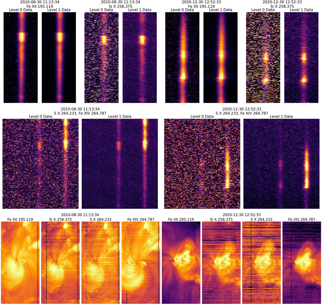
Figure 1. Data illustrating the EIS warm pixel problem. The top panels show EIS Level 0 and Level 1 exposures from early in the mission (left, 2010) and later in the mission (right, 2020). Level 0 data are the raw data telemetered from the spacecraft. The Level 1 data have had the warm pixels removed and replaced with interpolated values. In these images the X dimension is wavelength and the Y dimension is position along the EIS slit. The bottom panels show the rasters formed by integrating over the spectral dimension in the exposures. Residual warm pixels not removed in the current processing lead to the strong horizontal banding seen in the fainter regions of the rasters.

2.1 Synthetic EIS data

The development of machine learning algorithms for denoising EIS observations is complicated by the lack of noise-free images. The number of warm pixels early in the mission was relatively small, but still non-trivial. To address this, we have developed synthetic datasets with and without warm pixels that have the characteristics of EIS observations. These synthetic datasets consist of two key components: synthetic spectra that attempt to mimic the spectral features of EIS data, and synthetic dark images that have properties similar to what is observed on orbit, including the warm pixels.

The synthetic spectra are computed by combining active region and quiet sun differential emission measures from Warren et al. (2001) with the CHIANTI atomic database (Dere et al., 1997; 2023). These synthetic spectra are then convolved with the EIS instrument response function (see Lang et al., 2006; Warren et al., 2014 for details) to produce synthetic EIS exposures in the same units as those in the Level 0 data. We then generate a random function that mimics the variation of the solar signal along the slit and use this to create a mixture of active region and quiet sun spectra at each position.

As we will see, very high intensity features proved difficult for the model to reproduce. To help address this, we have also added a Gaussian to the active region spectrum to mimic the presence of bright points in the data. The Gaussian has a width of 2–$4^{\prime \prime }$ and is placed at a random position along the slit. This component is derived from the flare differential emission measure distributed with CHIANTI.

To create some variation in the synthetic spectra we chose different line widths for each feature: 60 mÅ for quiet sun, 66 mÅ for active regions, and 72 mÅ for the flare component. Further, abundance variations will also drive differences in relative line intensities. To mimic this we have chosen photospheric abundances for the quiet sun and bright point components and coronal abundances for the active region component.

The synthetic spectra along the slit are computed using

$\begin{array}{cc}\hfill s\left(\lambda ,y\right)=& \left(1-f_{ar}\left(y\right)\right)s_{qs}\left(\lambda \right)+f_{ar}\left(y\right)s_{ar}\left(\lambda \right)+\hfill \\ \hfill & f_{fl}\left(y\right)s_{fl}\left(\lambda \right),\hfill \end{array}$

where $f_{ar}(y)$ is the fraction of the active region spectrum at position $y$, and $s_{qs}(\lambda )$ and $s_{ar}(\lambda )$ are the quiet sun and active region spectra, respectively. The functions $f_{fl}(y)$ and $s_{fl}(\lambda )$ represent the flare contribution. After the synthetic spectra are computed in physical units, they are convolved with the EIS instrument response function (the effective area) to produce synthetic exposures in “data numbers” — the units returned by the detector electronics. Note that the EIS electronics return 14 bit integers (0 – 16,384). We then add Poisson noise to the synthetic exposure.

These synthetic exposures lack two essential features of the actual EIS data: the background and the warm pixels. The background is the sum of the pedestal added by the analog to digital converter of the camera electronics and the detector dark current. The background and the warm pixels are both included in the dark images that are taken with the shutter closed. To mimic the dark images, we have computed histograms from representative EIS dark observations and used the Python SciPy.stats method rv_histogram to generate random numbers that have the same distribution as the dark images. We then reshape the random numbers to the same dimensions as the synthetic exposures and add them together. Representative synthetic dark images are shown in Figure 2. We note that each realization of the synthetic dark images will have a histogram that is consistent with the real dark images, but the individual warm pixels will be in random locations. This helps the model to generalize to arbitrary real data.

Figure 2

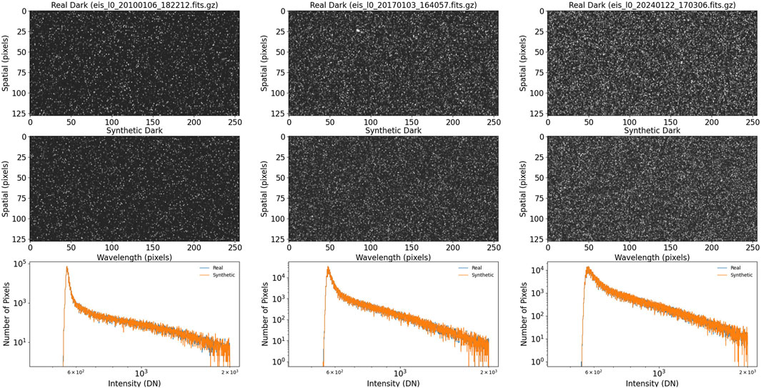
Figure 2. Real and synthetic dark images from various times in the mission. The bottom panels show the histograms for real and synthetic darks, which match very closely.

An example of the synthetic data is shown in Figure 3. For this example we have chosen the same synthetic exposure and combined it with synthetic darks from three different years, which illustrates the impact of the increasing warm pixel count on the observed spectra.

Figure 3

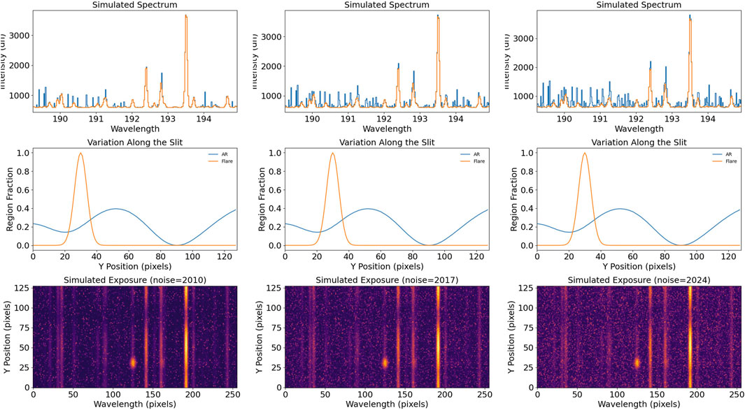
Figure 3. Examples of synthetic EIS exposures. The same synthetic exposure has been combined with synthetic darks from three different years. The top panels show representative spectra, The middle panels show the contribution of the active region and flare spectra to the variation of intensity along the slit, and the bottom panels show the exposures.

There are some differences between the synthetic and real data that we have not addressed. Perhaps most significantly, the synthetic data does not include strong variations in line widths or shifts. On the Sun these properties are a function of temperature (e.g., Chae et al., 1998b; a) and are also likely to vary by feature. A more subtle difference is that many physical processes and instrumental effects are likely to produce non-Gaussian line profiles (see Mandage and Bradshaw, 2020 and the references therein for a comprehensive discussion of this issue). As discussed in the next section, the model emphasizes local information and sees profiles at arbitrary locations, suggesting that these deficiencies in the synthetic data are acceptable. The application of the model to real data supports this. Future studies will include more detailed analysis of specific features.

3 Denoising architecture

3.1 Architecture

Our methodology employs the Conditional Generative Adversarial Network (cGAN) framework, drawing significant inspiration from the pioneering work of Isola et al. (2017).

A cGAN extends the traditional GAN framework by incorporating additional input information, enabling the generation of outputs conditioned on specific inputs. In our methodology, the cGAN leverages this conditioning mechanism to denoise noisy EIS images effectively. Unlike standard GANs, where the generator and discriminator operate solely on the input to generate images, the cGAN integrates auxiliary information — in this case, the noisy EIS image — into both the generator and discriminator. This conditioning ensures that the generator produces denoised images aligned with the corresponding noisy input, and the discriminator evaluates the generated outputs relative to the noisy input and ground-truth clean images. The overall architecture and interaction between these components are depicted in Figure 4.

Figure 4

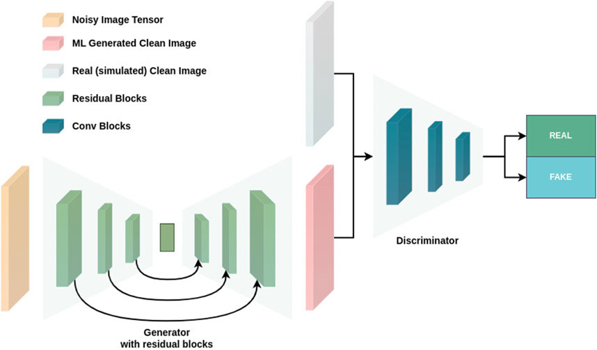
Figure 4. The architecture of the proposed model.

In this context, a clean, noise-free image from the ground truth dataset is denoted as a real image. A “fake” image is a denoised image produced by the generator. The discriminator’s goal is to distinguish between these two categories.

The generator employs a U-Net configuration, a well-established architecture for image-to-image translation tasks (Ronneberger et al., 2015; Zhou et al., 2019). A U-Net consists of an encoder-decoder structure with skip connections that preserve spatial information by directly connecting corresponding layers in the encoder and decoder with multiple residual blocks (He et al., 2016). Each residual block comprises a convolutional layer followed by a max-pooling layer, enabling multi-scale feature extraction. Batch normalization and dropout are integrated into the generator architecture to improve stability and mitigate overfitting, consistent with best practices in generative modeling (Kurach et al., 2018; Srivastava et al., 2014).

Mathematically, the discriminator, denoted as $D(x,y)$, takes an input pair $(x,y)$, where $x$ is the noisy input image and $y$ is either the ground truth clean image or the generator’s output. The discriminator learns a mapping $D:(x,y)\to [\mathrm{0,1}]$, assigning a higher score if $y$ corresponds to a real image and a lower score otherwise.

The discriminator diverges from the conventional setup by operating conditionally, assessing the correspondence between a noisy input and its paired denoised image. Instead of simply determining whether an image is real or fake, the discriminator evaluates whether the generated denoised image is consistent with the noisy input and comparable to the ground-truth clean image. For each noisy input, the discriminator is presented with two pairs: one combining the noisy input with its generator-produced output, and another pairing the noisy input with the ground-truth clean image. This conditional evaluation enhances the discriminator’s ability to guide the generator toward producing realistic, high-quality denoised outputs. The discriminator’s detailed structure is illustrated in Figure 4.

The interplay between the generator and discriminator follows the min-max adversarial paradigm intrinsic to GAN training. The generator is trained to produce denoised images that are indistinguishable from ground-truth clean images, while the discriminator continuously refines its capacity to distinguish between generated and authentic images. This adversarial dynamic drives the generator to progressively improve its denoising performance, resulting in outputs that are visually and quantitatively superior.

3.2 Loss

The cGAN model employs two primary loss functions: the GAN Loss and the Conditional Loss, which together guide the generator and discriminator during training.

GAN Loss: The GAN Loss is the traditional adversarial loss that drives the discriminator to distinguish between real and generated images. Simultaneously, it incentivizes the generator to produce outputs that are indistinguishable from real images. The adversarial loss is given by:

$\begin{array}{cc}\hfill {\mathcal{L}}_{\mathit{GAN}}\left(G,D\right)=& {\mathbb{E}}_{x,y}\left[\log D\left(x,y\right)\right]\hfill \\ \hfill & +{\mathbb{E}}_x\left[\log \left(1-D\left(x,G\left(x\right)\right)\right)\right]\hfill \end{array}$

where $G(x)$ represents the generator’s output for input $x$, and $D(x,y)$ is the discriminator’s probability that $y$ is a real image.

Conditional Loss: To ensure that the denoised image retains the structural and content-based characteristics of the input noisy image, we incorporate a conditional loss. This loss penalizes deviations between the generated denoised image and the ground-truth clean image at the pixel level. Using the $L_1$ distance, it is defined as:

${\mathcal{L}}_{\text{Conditional}}\left(G\right)={\mathbb{E}}_{x,y}\left[\Vert y-G\left(x\right){\Vert }_1\right]$

where $\Vert y-G(x){\Vert }_1$ represents the sum of absolute pixel-wise differences.

Total Loss: The total loss for training the cGAN model is a weighted combination of the GAN Loss and the Conditional Loss:

${\mathcal{L}}_{\text{Total}}\left(G,D\right)={\mathcal{L}}_{\mathit{GAN}}\left(G,D\right)+\lambda {\mathcal{L}}_{\text{Conditional}}\left(G\right)$

where $\lambda$ is a hyperparameter that balances the two loss components. Unlike its conventional use for wavelength notation, here $\lambda$ is a tunable weight controlling the relative contribution of conditional loss.

3.3 Training procedure

Training a conditional GAN begins by inputting a noisy image into the generator, which attempts to produce a denoised version. The generated denoised image, along with the corresponding noisy input, is evaluated by the discriminator, which determines whether the generated output is real or fake. In each iteration, the discriminator is also presented with pairs of the noisy input and the ground-truth clean image. The discriminator’s objective is to assign a high score to real denoised images and a low score to those produced by the generator. Feedback from the discriminator is then used to update the weights of both the generator and discriminator using their respective loss functions.

The U-Net-structured generator uses three convolutional blocks each consisting of two convolutional layers followed by LeakyReLU activations. LeakyReLU is an activation function similar to ReLU but allows small negative values instead of setting them to zero, thereby preventing dying neurons and improving gradient flow (Maas et al., 2013; Xu et al., 2020). The architecture includes a down-sampling block ($1\to 64$ channels) with a residual block ($64\to 64$ channels) for feature refinement, followed by an additional down-sampling block ($64\to 128$ channels) (He et al., 2016). An up-sampling block ($128\to 64$ channels) uses transposed convolutions to reconstruct the image, while skip-connections between down-sampling and up-sampling layers ensure the preservation of spatial details (Zhou et al., 2019). The final layer ($64\to 1$ channels) produces the denoised image.

The discriminator used in this denoiser is a convolutional neural network with four convolutional layers that progressively reduce spatial dimensions. The first layer ($1\to 10$ channels) uses a kernel size of $4\times 4$ and stride 2, followed by intermediate layers ($10\to 4\to 4$ channels) with BatchNorm and Dropout for regularization. The final layer ($4\to 1$ channels) outputs a classification score through a Sigmoid activation, determining whether the input is real or fake.

For the EIS images, obtaining true noise-free data is not possible. As described in Section 2.1, synthetic clean data is generated to mimic true noise-free images, while synthetic noisy data is designed to replicate the noise observed in warm pixels. This synthetic dataset is divided into three parts: training, hyperparameter tuning, and validation.

Synthetic images were generated for the full $1024\times 1024$ size of the EIS detectors, but the model was trained on smaller $64\times 128$ patches randomly sampled from the full images. This approach was adopted because only small regions around spectral lines are typically saved and transmitted to the ground to conserve telemetry. Training on small patches better reflects real observational conditions, accelerates training, and allows the use of GPUs with limited memory. Random patch selection ensures the model generalizes to any part of the detector.

A total of 50,000 training pairs, 5,000 validation pairs, and 5,000 testing pairs were generated. The training set was used for regular training, the validation set was used to tune the hyperparameters, and the test set was used to determine the final performance. The model was trained for 1,000 epochs with a batch size of 32, although significant improvements were mainly observed within the first few hundred epochs. The Adam optimizer (Kingma and Ba, 2014) was employed with fixed learning rates of 0.00020 and 0.00025 for the generator and discriminator, respectively. The implementation was carried out using the PyTorch framework.

3.4 Training analysis

The inception score (IS) is a popular metric used in image generation tasks (Chong and Forsyth, 2020). It measures the diversity and quality of generated images by evaluating the entropy of predictions made by a pre-trained classifier. While this metric is useful for a general generative task, it allows high variability in the outputs making them unsuitable for our task. Thus, we selected the pixel-wise percent difference as our primary evaluation metric.

Pixel-wise RMSE percent difference is computed as:

$P_{\text{RMSE}}=\sqrt{\frac{1}{N}{\displaystyle \sum _{i=1}^N}{\left(\frac{I_{\text{gen}}\left(i\right)-I_{\text{gt}}\left(i\right)}{I_{\text{gt}}\left(i\right)}\right)}^2}\times 100$

where $I_{\text{gen}}(i)$ and $I_{\text{gt}}(i)$ are pixel intensities of the generated and ground-truth images, respectively, and $N$ is the total number of pixels.

We monitored the model’s performance by tracking training and validation losses across epochs. The training loss encompasses both GAN and Conditional losses, whereas the validation loss is determined solely through the pixel-wise percent difference between the generated output and the real noise-free image. So, numerically they are a bit different. However, their growth and trends offer meaningful insights into the model. We saw a steady decline in the training loss indicating continual model learning. Similarly, the consistent decrease in the validation loss indicates the model’s strong generalization to unseen data. It is worth noting that occasionally the validation loss is lower than the training loss due to the differences in computing methods.

Examples of the model applied to the test set are given in Figure 5. Here the input noisy image, the ground truth clean image, and the model’s output are shown. The bottom panels show the percent difference between the model’s output and the ground truth image as well as representative spectra. The model is quite effective at removing the noise, but it does not always reproduce the sharpest peaks in the data. Figure 5 highlights discrepancies in bright points. The magnitude of these discrepancies varies depending on intensity, with errors typically within 5%–10% for bright features. These discrepancies arise due to limited high-intensity training samples. Future improvements could incorporate weighted loss functions to focus more on high-intensity structures. The number of warm pixels in EIS images varies over time due to detector aging. Our training/validation/testing datasets are synthetic and use variable noise levels to capture this variability, ensuring robustness.

Figure 5

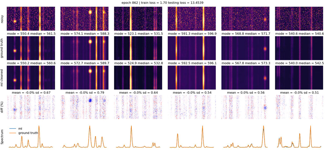
Figure 5. Examples of noisy, ground truth, and cleaned images from the testing set. The bottom panels show maps of percent difference between the cleaned and ground truth images as well as representative spectra.

Finally, Figure 6 shows examples of the model applied to the validation set, which was not used in model training or hyper-parameter tuning. As would be expected from the volume of training data, the model performs very well on the validation set, although the discrepancies at high intensities are still present.

Figure 6

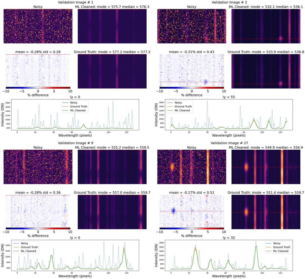
Figure 6. Examples of the model applied to the validation set, which was not used in model training or hyper-parameter optimization. The input noisy image, the ground truth clean image, and the model’s output are shown. The bottom panels show the percent difference between the model’s output and the ground truth image as well as representative spectra. The model is quite effective at removing the noise, but it does not always reproduce the sharp peaks in the data.

In Figure 6, color bars have been added to the percentage difference panels to visualize error magnitudes. The blue spectral curves correspond to specific $y$-pixel locations, and an annotation has been added to clarify whether they represent single-pixel or averaged spectra.

4 Application to real data

The application of the model to real EIS data is complicated by the fact that EIS observations typically consist of small spectral windows of varying size read out from the full detector. These windows typically contain only a single spectral line, but some contain multiple spectral features (see Figure 1). To apply the model to arbitrary spectral windows, we first pad the data to be a multiple of $64\times 128$ (the size of the training data) and then apply the model to each $64\times 128$ patch. To mitigate edge effects, we apply the model to patches shifted by two pixels both horizontally and vertically, resulting in 32 overlapping predictions for most pixel positions. We choose the median of these overlapping predictions to obtain the final result, as this approach effectively removes patch boundary artifacts. The denoised patches are then reassembled into the full image.

Figure 7 shows an example of the model applied to real EIS data. This observation was chosen because it contains a mix of bright and dark regions and has no missing exposures. These data were taken 23-Oct-2024 using 40 s exposures and the $2^{\prime \prime }$ slit. The spectral profiles and intensities along the slit (shown in the right panels of this figure) clearly show a reduction in noise in both the spectral and spatial directions. Comparing the rasters formed by simply summing over the spectral windows shows that the model is quite effective at removing the warm pixels. Much of horizontal banding evident in images is removed in the ML version of the rasters. The improvement is somewhat limited for the strong Fe XII line, but is more pronounced for the weaker Fe XI and Fe X lines.

Figure 7

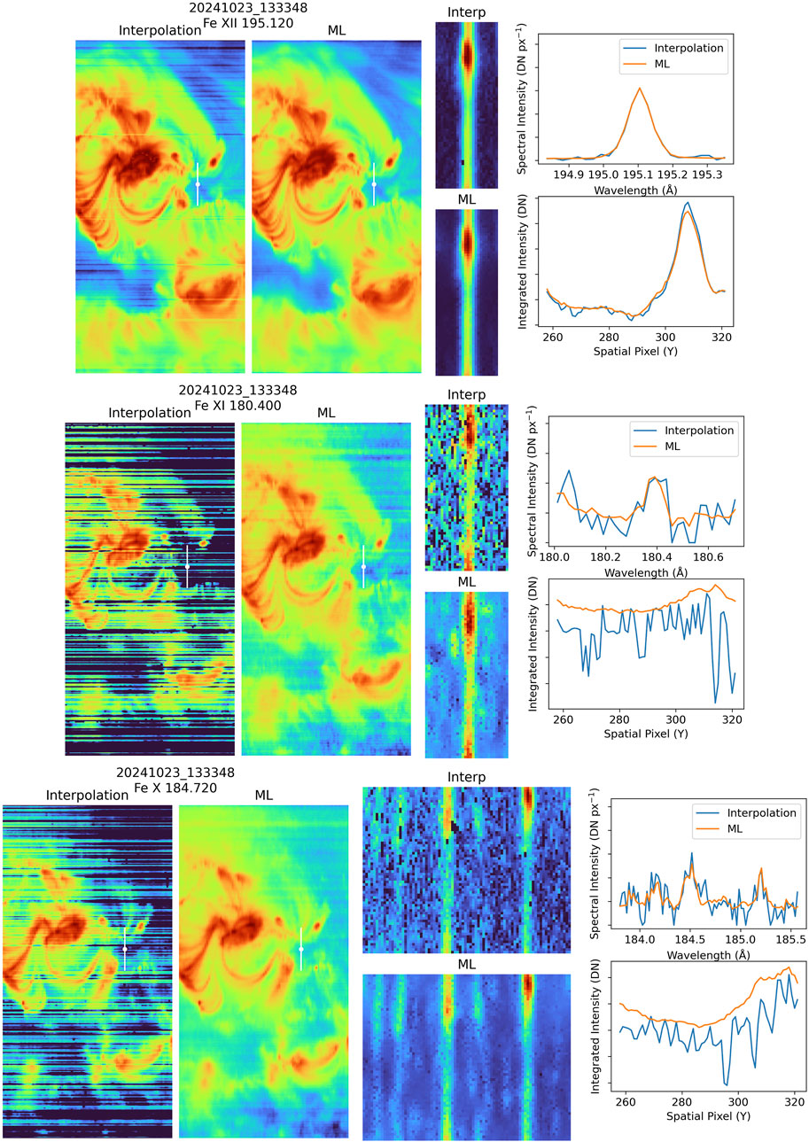
Figure 7. An example of applying the model to real EIS data. The left panels show the raster images, the middle panels show the exposures, and the right panels show representative spectra (from the point indicated by the dot) and integrated intensities (from the region indicated by the line). “Interpolation” refers to the current interpolation method, and “ML” refers to the machine learning model. Here the intensities are computed by simply summing over the spectral window. The machine learning model is quite effective at removing the warm pixels. The improvement is somewhat limited for the strong Fe XII line, but is more pronounced for the weaker Fe XI and Fe X lines.

However, it is important to note that most EIS analysis generally relies on fitting Gaussian profiles to the spectral lines, and not on summing over the spectral dimension. To test the model’s effectiveness in this context, we have created updated HDF5 data files compatible with the EISPACsoftware (Weberg et al., 2023), which provides the capability for spectral fitting. Figures 8, 9 shows examples of the model applied to these data and analyzed with EISPAC. To use the model output in EISPAC we convert the processed data from units of DN to counts. EISPAC then applies the pre-flight calibration to convert to physical units. In this context the ML model shows only a modest improvement over the current interpolation method. The ML versions of the intensity rasters are very similar to those produced by simply summing over the spectral dimension. The spectral fitting of the current data also produces a similar result, with there only being a modest reduction in the horizontal banding. The maps of the line shift and line width are also very similar for both the current and ML versions of the data, with strong horizontal banding seen in both sets of images.

Figure 8

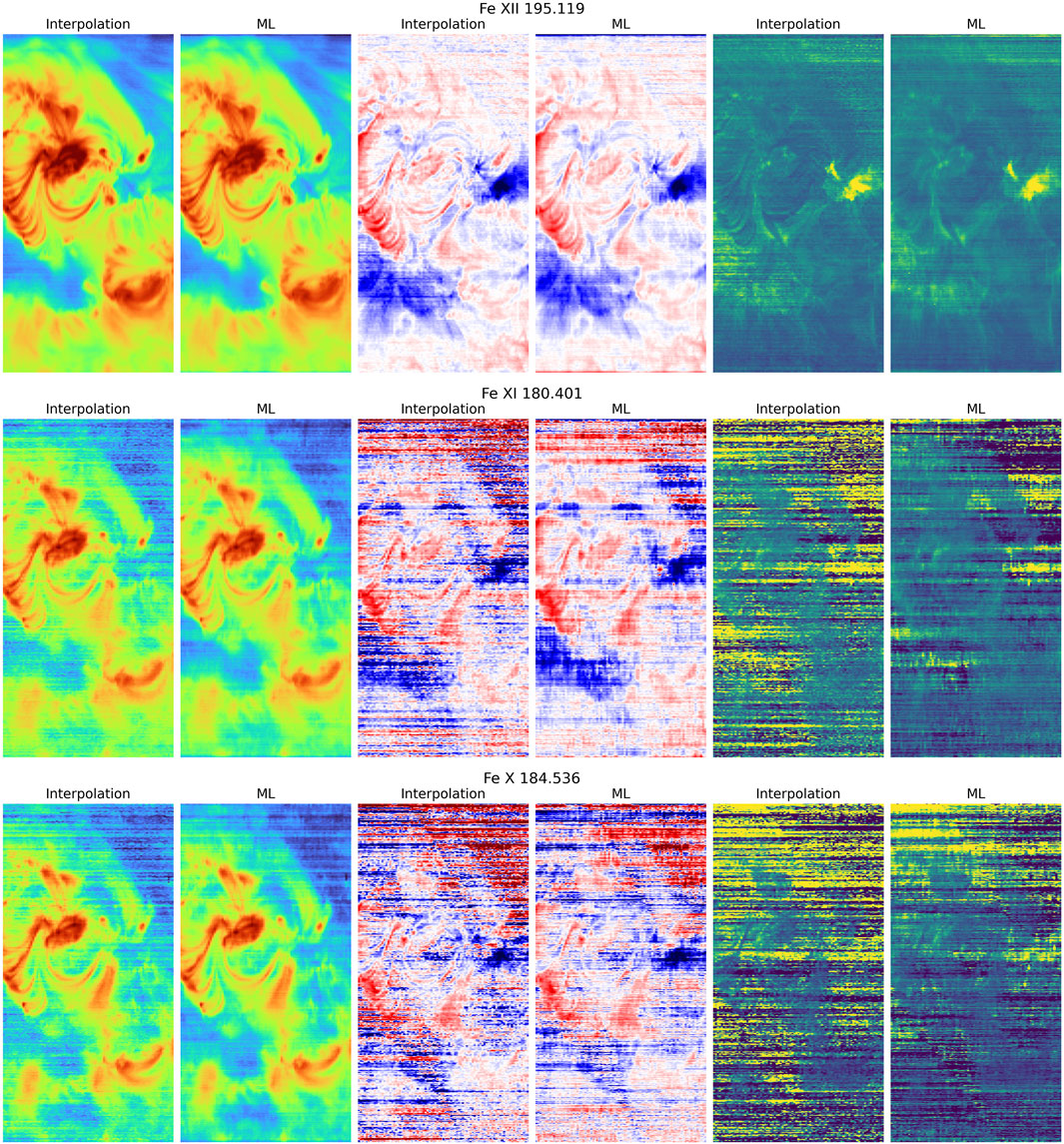
Figure 8. Comparisons of fitting Gaussians to the EIS data using the current interpolation method and the machine learning model. The line intensity, line shift, and line width are shown. The machine learning model produces a modest improvement over the current interpolation method.

Figure 9

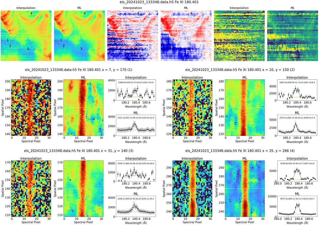
Figure 9. Examples of weak spectral features observed with EIS in Fe XI 180.401 Å. The top panels show a small cutout of the intensities, Doppler shifts, and line intensities from the larger rasters in Figure 8. The bottom panels show small regions of the detector exposure as well as some representative line profiles. The line profiles plots also show Gaussian fits and the corresponding fit parameters. The units are erg ${\mathrm{c}\mathrm{m}}^{-2}$ ${\mathrm{s}}^{-1}$ ${\mathrm{s}\mathrm{r}}^{-1}$ for the intensity, km ${\mathrm{s}}^{-1}$ for the Doppler shift, and mÅ for the width. As suggested by Figure 8, the machine learning model produces a dramatic improvement in the signal-to-noise in the profile, but only modest improvement over the current interpolation method in the final fit parameters.

5 Conclusion

Our cGAN-based approach to image denoising of EIS images has shown considerable potential in handling the complex noise characteristics inherent in the EIS data. The strategic integration of the U-Net architecture and the conditional learning framework into our cGAN model has enabled the generation of denoised images that maintain a high degree of fidelity to the real data. While the model excels in general noise reduction and retaining image content, it appears to offer only a modest improvement over the current interpolation method when it comes to Gaussian line fitting. It is also challenged in accurately capturing high-intensity peaks in some cases.

Since thresholding is used in the interpolation method for denoising, the persistence of warm pixels in the current processing pipeline is easy to understand. How these residual warm pixels persist in the machine learning algorithm is not clear. It is possible that at sufficiently low amplitudes, the warm pixels are difficult to distinguish from the Poisson noise.

While the model may appear to make only modest improvements over the current processing method, it may pave the way for making use of longer exposures to improve the observation of fainter features. Recall that the signal in the warm pixels increases with time, largely negating the benefits of longer exposures. With its improved ability to extract the signal from the warm pixel noise, it seems likely that the model will be more effective in this context.

The fitting of the spectral features is not the final goal of EIS data analysis. The next step in the testing of this software will be to use the fitted profiles to infer the physical properties of the solar atmosphere. Future work with the ML model will involve performing detailed analysis using both the current methods and this new, machine learning-based processing.

The ML denoising model is not publicly distributed at this time. Since the ML model works on the Level 0 files and requires pyTorch, we are working to distribute it as a standalone package separate from EISPAC.

Data availability statement

The raw data supporting the conclusions of this article will be made available by the authors, without undue reservation.

Author contributions

MR: Conceptualization, Data curation, Formal Analysis, Investigation, Methodology, Software, Validation, Visualization, Writing – original draft, Writing – review and editing. HW: Conceptualization, Data curation, Formal Analysis, Funding acquisition, Investigation, Methodology, Project administration, Resources, Software, Supervision, Validation, Visualization, Writing – original draft, Writing – review and editing.

Funding

The author(s) declare that financial support was received for the research and/or publication of this article. This research was funded by NASA’s Hinode program.

Acknowledgments

The authors would like to thank Al Amin Hosain for his work on an earlier version of this project.

Conflict of interest

The authors declare that the research was conducted in the absence of any commercial or financial relationships that could be construed as a potential conflict of interest.

Generative AI statement

The author(s) declare that no Generative AI was used in the creation of this manuscript.

Publisher’s note

All claims expressed in this article are solely those of the authors and do not necessarily represent those of their affiliated organizations, or those of the publisher, the editors and the reviewers. Any product that may be evaluated in this article, or claim that may be made by its manufacturer, is not guaranteed or endorsed by the publisher.

Footnotes

¹https://solarb.mssl.ucl.ac.uk/SolarB/eis_docs/eis_notes/06_HOT_WARM_PIXELS/eis_swnote_06.pdf

²https://solarb.mssl.ucl.ac.uk/SolarB/eis_docs/eis_notes/13_INTERPOLATION/eis_swnote_13.pdf

³https://solarb.mssl.ucl.ac.uk/SolarB/eis_docs/eis_notes/24_COSMIC_RAYS/eis_swnote_24.pdf

⁴https://solarb.mssl.ucl.ac.uk/SolarB/eis_docs/eis_notes/08_COMA/eis_swnote_08.pdf

References

Abdal, R., Qin, Y., and Wonka, P. (2019). “Image2stylegan: how to embed images into the stylegan latent space?,” in Proceedings of the IEEE/CVF international conference on computer vision, Seoul, Korea (South), 27 October 2019 - 02 November 2019, 4432–4441.

Google Scholar

Al-Janabi, K., Antolin, P., Baker, D., Bellot Rubio, L. R., Bradley, L., Brooks, D. H., et al. (2019). Achievements of Hinode in the first eleven years. PASJ 71, R1. doi:10.1093/pasj/psz084

CrossRef Full Text | Google Scholar

Baraniuk, R. G. (1999). Optimal tree approximation with wavelets. Wavelet Appl. Signal Image Process. VII (SPIE) 3813, 196–207. doi:10.1117/12.366780

CrossRef Full Text | Google Scholar

BenMoussa, A., Gissot, S., Schühle, U., Del Zanna, G., Auchère, F., Mekaoui, S., et al. (2013). On-orbit degradation of solar instruments. Sol. Phys. 288, 389–434. doi:10.1007/s11207-013-0290-z

CrossRef Full Text | Google Scholar

Brooks, D. H., Warren, H. P., and Ugarte-Urra, I. (2012). Solar coronal loops resolved by Hinode and the solar dynamics observatory. ApJL 755, L33. doi:10.1088/2041-8205/755/2/L33

CrossRef Full Text | Google Scholar

Bui, T. D., and Chen, G. (1998). Translation-invariant denoising using multiwavelets. IEEE Trans. signal Process. 46, 3414–3420. doi:10.1109/78.735315

CrossRef Full Text | Google Scholar

Cao, Y., Liu, B., Long, M., and Wang, J. (2018). “Hashgan: deep learning to hash with pair conditional wasserstein gan,” in Proceedings of the IEEE conference on computer vision and pattern recognition. 18-23 June 2018. Salt Lake City, UT, USA. 1287–1296. doi:10.1109/cvpr.2018.00140

CrossRef Full Text | Google Scholar

Chae, J., Schühle, U., and Lemaire, P. (1998a). SUMER measurements of nonthermal motions: constraints on coronal heating mechanisms. ApJ 505, 957–973. doi:10.1086/306179

CrossRef Full Text | Google Scholar

Chae, J., Yun, H. S., and Poland, A. I. (1998b). Temperature dependence of ultraviolet line average Doppler shifts in the quiet sun. ApJSS 114, 151–164. doi:10.1086/313064

CrossRef Full Text | Google Scholar

Chen, Z., Zeng, Z., Shen, H., Zheng, X., Dai, P., and Ouyang, P. (2020). Dn-gan: denoising generative adversarial networks for speckle noise reduction in optical coherence tomography images. Biomed. Signal Process. Control 55, 101632. doi:10.1016/j.bspc.2019.101632

CrossRef Full Text | Google Scholar

Chong, M. J., and Forsyth, D. (2020). “Effectively unbiased fid and inception score and where to find them,” in Proceedings of the IEEE/CVF conference on computer vision and pattern recognition, Seattle, WA, USA, 13-19 June 2020, 6070–6079.

Google Scholar

Coifman, R. R., and Donoho, D. L. (1995). Translation-invariant de-noising. Springer.

Google Scholar

Creswell, A., White, T., Dumoulin, V., Arulkumaran, K., Sengupta, B., and Bharath, A. A. (2018). Generative adversarial networks: an overview. IEEE signal Process. Mag. 35, 53–65. doi:10.1109/msp.2017.2765202

CrossRef Full Text | Google Scholar

Culhane, J. L., Harra, L. K., James, A. M., Al-Janabi, K., Bradley, L. J., Chaudry, R. A., et al. (2007). The EUV imaging spectrometer for Hinode. Sol. Phys. 243, 19–61. doi:10.1007/s01007-007-0293-1

CrossRef Full Text | Google Scholar

Dere, K. P., Del Zanna, G., Young, P. R., and Landi, E. (2023). CHIANTI-an atomic database for emission lines. XVII. Version 10.1: revised ionization and recombination rates and other updates. ApJSS 268, 52. doi:10.3847/1538-4365/acec79

CrossRef Full Text | Google Scholar

Dere, K. P., Landi, E., Mason, H. E., Monsignori Fossi, B. C., and Young, P. R. (1997). CHIANTI - an atomic database for emission lines. Astronomy Astrophysics Suppl. Ser. 125, 149–173. doi:10.1051/aas:1997368

CrossRef Full Text | Google Scholar

Donoho, D. L. (1995). De-noising by soft-thresholding. IEEE Trans. Inf. theory 41, 613–627. doi:10.1109/18.382009

CrossRef Full Text | Google Scholar

Fan, L., Zhang, F., Fan, H., and Zhang, C. (2019). Brief review of image denoising techniques. Vis. Comput. Industry, Biomed. Art 2, 7–12. doi:10.1186/s42492-019-0016-7

PubMed Abstract | CrossRef Full Text | Google Scholar

Fodor, I. K., and Kamath, C. (2003). Denoising through wavelet shrinkage: an empirical study. J. Electron. Imaging 12, 151–160. doi:10.1117/1.1525793

CrossRef Full Text | Google Scholar

Golub, L., Deluca, E., Austin, G., Bookbinder, J., Caldwell, D., Cheimets, P., et al. (2007). The X-ray telescope (XRT) for the Hinode mission. Sol. Phys. 243, 63–86. doi:10.1007/s11207-007-0182-1

CrossRef Full Text | Google Scholar

Goodfellow, I., Pouget-Abadie, J., Mirza, M., Xu, B., Warde-Farley, D., Ozair, S., et al. (2020). Generative adversarial networks. Commun. ACM 63, 139–144. doi:10.1145/3422622

CrossRef Full Text | Google Scholar

Gupta, K., and Gupta, S. (2013). Image denoising techniques-a review paper. IJITEE 2, 6–9.

Google Scholar

He, K., Zhang, X., Ren, S., and Sun, J. (2016). “Deep residual learning for image recognition,” in Proceedings of the IEEE conference on computer vision and pattern recognition, Las Vegas, NV, USA, 27-30 June 2016, 770–778.

Google Scholar

Isola, P., Zhu, J.-Y., Zhou, T., and Efros, A. A. (2017). “Image-to-image translation with conditional adversarial networks,” in Proceedings of the IEEE conference on computer vision and pattern recognition, Honolulu, HI, USA, 21-26 July 2017, 1125–1134.

Google Scholar

Kim, T., Cha, M., Kim, H., Lee, J. K., and Kim, J. (2017). “Learning to discover cross-domain relations with generative adversarial networks,” in International conference on machine learning (Sydney, Australia: PMLR), 1857–1865.

Google Scholar

Kingma, D. P., and Ba, J. (2014). Adam: a method for stochastic optimization. arXiv preprint arXiv:1412.6980.

Google Scholar

Kurach, K., Lucic, M., Zhai, X., Michalski, M., and Gelly, S. (2018). The gan landscape: losses, architectures, regularization, and normalization

Google Scholar

Lang, J., Kent, B. J., Paustian, W., Brown, C. M., Keyser, C., Anderson, M. R., et al. (2006). Laboratory calibration of the extreme-ultraviolet imaging spectrometer for the solar-B satellite. Appl. Opt. 45, 8689–8705. doi:10.1364/AO.45.008689

PubMed Abstract | CrossRef Full Text | Google Scholar

Lang, M., Guo, H., Odegard, J. E., Burrus, C. S., and Wells Jr, R. O. (1995). Nonlinear processing of a shift-invariant discrete wavelet transform (dwt) for noise reduction. Wavelet Appl. II (SPIE) 2491, 640–651. doi:10.1117/12.205427

CrossRef Full Text | Google Scholar

Li, Y., Zhang, K., Shi, W., Miao, Y., and Jiang, Z. (2021). A novel medical image denoising method based on conditional generative adversarial network. Comput. Math. Methods Med. 2021, 1–11. doi:10.1155/2021/9974017

PubMed Abstract | CrossRef Full Text | Google Scholar

Li, Z., Zhou, S., Huang, J., Yu, L., and Jin, M. (2020). Investigation of low-dose ct image denoising using unpaired deep learning methods. IEEE Trans. Radiat. plasma Med. Sci. 5, 224–234. doi:10.1109/trpms.2020.3007583

PubMed Abstract | CrossRef Full Text | Google Scholar

Maas, A. L., Hannun, A. Y., and Ng, A. Y. (2013). Rectifier nonlinearities improve neural network acoustic models. Proc. icml (Atlanta, GA) 30 (3).

Google Scholar

Mallat, S., and Hwang, W. L. (1992). Singularity detection and processing with wavelets. IEEE Trans. Inf. theory 38, 617–643. doi:10.1109/18.119727

CrossRef Full Text | Google Scholar

Mandage, R. S., and Bradshaw, S. J. (2020). Asymmetries and broadenings of spectral lines in strongly charged iron produced during solar flares. ApJ 891, 122. doi:10.3847/1538-4357/ab7340

CrossRef Full Text | Google Scholar

Motwani, M. C., Gadiya, M. C., Motwani, R. C., and Harris, F. C. (2004). Survey of image denoising techniques. Proc. GSPX 27, 27–30.

Google Scholar

Ronneberger, O., Fischer, P., and Brox, T. (2015). “U-net: convolutional networks for biomedical image segmentation,” in Medical image computing and computer-assisted intervention–MICCAI 2015: 18th international conference, Munich, Germany, October 5-9, 2015, proceedings, part III 18 (Springer), 234–241.

Google Scholar

Srivastava, N., Hinton, G., Krizhevsky, A., Sutskever, I., and Salakhutdinov, R. (2014). Dropout: a simple way to prevent neural networks from overfitting. J. Mach. Learn. Res. 15, 1929–1958.

Google Scholar

Tian, C., Fei, L., Zheng, W., Xu, Y., Zuo, W., and Lin, C.-W. (2020a). Deep learning on image denoising: an overview. Neural Netw. 131, 251–275. doi:10.1016/j.neunet.2020.07.025

PubMed Abstract | CrossRef Full Text | Google Scholar

Tian, C., Xu, Y., Li, Z., Zuo, W., Fei, L., and Liu, H. (2020b). Attention-guided cnn for image denoising. Neural Netw. 124, 117–129. doi:10.1016/j.neunet.2019.12.024

PubMed Abstract | CrossRef Full Text | Google Scholar

Warren, H. P., Mariska, J. T., and Lean, J. (2001). A new model of solar EUV irradiance variability: 1. Model formulation. J. Geophys. Res. 106, 15745–15757. doi:10.1029/2000JA000282

CrossRef Full Text | Google Scholar

Warren, H. P., Ugarte-Urra, I., and Landi, E. (2014). The absolute calibration of the EUV imaging spectrometer on Hinode. ApJSS 213, 11. doi:10.1088/0067-0049/213/1/11

CrossRef Full Text | Google Scholar

Weberg, M., Warren, H., Crump, N., and Barnes, W. (2023). EISPAC - the EIS Python analysis code. J. Open Source Softw. 8, 4914. doi:10.21105/joss.04914

CrossRef Full Text | Google Scholar

Xu, J., Li, Z., Du, B., Zhang, M., and Liu, J. (2020). “Reluplex made more practical: leaky relu,” in 2020 IEEE Symposium on Computers and communications (ISCC), Rennes, France, 07-10 July 2020 (IEEE), 1–7.

CrossRef Full Text | Google Scholar

Yang, R., Yin, L., Gabbouj, M., Astola, J., and Neuvo, Y. (1995). Optimal weighted median filtering under structural constraints. IEEE Trans. signal Process. 43, 591–604. doi:10.1109/78.370615

CrossRef Full Text | Google Scholar

Yin, Z., Xia, K., He, Z., Zhang, J., Wang, S., and Zu, B. (2021). Unpaired image denoising via wasserstein gan in low-dose ct image with multi-perceptual loss and fidelity loss. Symmetry 13, 126. doi:10.3390/sym13010126

CrossRef Full Text | Google Scholar

Zahin, N. M., Rahman, M. M., and Mahmud, K. R. (2021). StructGAN: image restoration maintaining structural consistency using A two-step generative adversarial network. Ph.D. thesis (Gazipur, Bangladesh: Department of Computer Science and Engineering (CSE), Islamic University of Technology).

Google Scholar

Zhang, K., Zuo, W., Chen, Y., Meng, D., and Zhang, L. (2017). Beyond a Gaussian denoiser: residual learning of deep cnn for image denoising. IEEE Trans. image Process. 26, 3142–3155. doi:10.1109/tip.2017.2662206

PubMed Abstract | CrossRef Full Text | Google Scholar

Zhou, Z., Siddiquee, M. M. R., Tajbakhsh, N., and Liang, J. (2019). Unet++: redesigning skip connections to exploit multiscale features in image segmentation. IEEE Trans. Med. imaging 39, 1856–1867. doi:10.1109/tmi.2019.2959609

PubMed Abstract | CrossRef Full Text | Google Scholar