 Xuedong Feng
 Jian Yang
 Jacob Bortnik
 Chih-Ping Wang
 Jiang Liu
- 1Department of Earth and Space Sciences, Southern University of Science and Technology, Shenzhen, China
- 2Department of Atmospheric and Oceanic Sciences, University of California, Los Angeles, Los Angeles, CA, United States
- 3Department of Earth, Planetary, and Space Sciences, University of California, Los Angeles, Los Angeles, CA, United States
Bursty bulk flows (BBFs) play a crucial role in transporting energy, mass, and magnetic flux from the Earth’s magnetotail to the near-Earth region. However, their impulsive nature and small spatial scale pose significant difficulties for in-situ observations, given that only a handful number of spacecraft operate within the vast expanse of the magnetotail. Consequently, accurately predicting their behavior remains a challenging goal. In this study, we employ the XGBoost machine learning algotithm to predict the variation range of several essential BBF properties, including duration, magnetic field, plasma moments, and specific entropy parameters. The observed characteristics of a BBF are shaped by its formation in the downstream tail and its journey until it reaches the spacecraft. Therefore, we use both the background properties of the plasma sheet prior to the arrival of the BBF and the attributes of indirectly related variables during the BBF interval as inputs. Trained on 17 years of THEMIS data, we explore different input configurations. One approach involves incorporating optimal parameter combinations, utilizing as many input parameters as possible to predict upper and lower bounds of a target variable. Within this framework, we further apply the leave-one-feature-out method to quantitatively assess the contribution of each input, identifying the most dominant factor influencing BBFs in a statistical sense. Another approach involves cross-instrument prediction, leveraging measurements from a different payload. Our findings reveal that including observed background values enhances prediction accuracy by 10–20 percentage points. This study offers data-driven insights to improve BBF predictability, providing valuable guidance for future space weather monitoring and theoretical research.
1 Introduction
The plasma sheet in Earth’s magnetosphere is a highly dynamic region that plays a critical role in transporting energy and particles during geomagnetic active times (Angelopoulos et al., 1994). Within this region, bursty bulk flows (BBFs) —localized and transient elevation in ion bulk flow speed to the order of hundreds of km/s—are key to understanding how energy is transferred from the magnetotail to the inner magnetosphere (Angelopoulos et al., 1992). Numerous studies have highlighted the critical role of BBFs in the transport of mass, energy, and magnetic flux from the magnetotail to the near-Earth region during geomagnetic activity. Observational analyses, such as those by Nakamura et al. (2001), Nakamura et al. (2002), Nakamura et al. (2005), revealed that BBFs are closely associated with dipolarization fronts and plasma sheet thinning, underscoring their importance in magnetotail reconfiguration. Complementary investigations by Cao et al. (2013) and Yao et al. (2013) further established statistical relationships between BBFs and field-aligned currents or flow bursts, providing insight into their spatial and temporal properties. Forsyth et al. (2008) and Grocott et al. (2004) demonstrated how BBFs influence ionospheric signatures and substorm dynamics, while Henderson et al. (1998) connected BBFs with auroral intensifications. Together, these studies underscore the importance of accurately characterizing BBFs to improve our understanding of magnetospheric dynamics. BBFs are the observational counterpart of plasma-sheet bubbles, which are theoretically defined as depleted magnetic flux tubes containing lower entropy than their neighbors (e.g., Pontius and Wolf, 1990; Birn et al., 2004; Runov et al., 2017). The BBFs or bubbles are often created by magnetic reconnection events (Sitnov et al., 2005; Birn et al., 2011), but may also arise from other explosive magnetotail processes (e.g.,Yang et al., 2011; Hu et al., 2011; Sitnov et al., 2019). They can further lead to significant space weather phenomena, such as auroral intensification (Nishimura et al., 2010; Shi et al., 2012) and energetic particle flux enhancements in the inner magnetosphere (Ohtani et al., 2006; Yang et al., 2011).
Although statistical studies that incorporate a set of physical parameters and numerical simulations using advanced MHD or kinetic models have provided invaluable insights, predicting the characteristics of BBFs remains extremely challenging. This difficulty arises from the multiscale nature of magnetotail dynamics, limited observational coverage, and the complex interplay of physical processes driving BBF formation and evolution. Statistical analyses of BBFs involve a number of physical parameters – such as magnetic field, plasma bulk velocity, thermal pressure, temperature and number density – as well as other complex quantities such as magnetic flux transport, specific entropy, electric field and particle distribution functions (e.g., Ohtani, 2004; Liu et al., 2013; Runov et al., 2015; Runov et al., 2017). Like many other statistical approaches, the results often become heavily smoothed, providing only rough estimates of likely ranges. For instance, the left panels of Figure 1 (adapted from Ohtani, 2004) show aggregated measurements that obscure time variations during the BBF injection. Consequently, these statistics cannot yield reliable prediction results for any specific event.
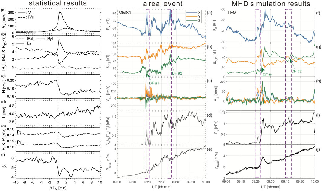
Figure 1. (Left panels, adapted from Figure 3 of Ohtani, 2004). Statistical results of a superposed epoch analysis of key quantities surrounding the arrival of BBFs from
Numerical simulations offer an alternative approach. Certain simulations aim to qualitatively explain the variability of BBFs but face considerable challenges in accurately replicating actual events. For instance, Chen and Wolf (1999) formulated an MHD theory to simulate BBF propagation, treating the moving flux tube as an infinitely thin filament within a 2D stationary medium in MHD equilibrium. Meanwhile, simulations employing the Rice Convection Model demonstrated an increase in energetic particle flux at geosynchronous orbit due to a BBF’s deep injection, generating a dipolarization front via coupling with a force equilibrium solver; however, these simulations omitted inertial effects (Yang et al., 2011). Birn et al. (2011) utilized a 3D one-fluid MHD code to study BBF propagation, observing damped oscillations in the near-Earth region. Yet, their model was confined to a rectangular box encompassing only the nightside region, with perfectly conducting boundaries, and the quantitative accuracy of their idealized simulations hinged on the selection of scaling constants. Other simulations incorporate solar wind conditions as inputs for global MHD codes, and may thereby deliver relatively satisfactory predictions (e.g., Ashour-Abdalla et al., 2011; Merkin et al., 2019). However, these simulations are computationally expensive, and the agreement between model and observation is usually limited to only a few events. An example in the center and right panels of Figure 1 [adapted from Merkin et al. (2019)] illustrates an overall good agreement but reveals discrepancies in the precise timing and magnitudes of key parameters.
Building upon prior research, recent advancements in artificial intelligence (AI) technology and an ever-expanding data pool now offer a more robust foundation for improving prediction (Camporeale, 2019; Bortnik et al., 2018). In this study, our ultimate goal is to provide reliable predictions of key BBF properties—such as mean, maximum, minimum and range—once a BBF occurs. This objective involves two main aspects.
First, we aim to maximize prediction accuracy by utilizing as many relevant input parameters as possible. To this end, we optimized the selection of input parameters by analyzing their distribution and relevance to BBF prediction using Kernel Density Estimation (Chen, 2017). We then employed eXtreme Gradient Boosting (XGBoost) (Chen and Guestrin, 2016), a powerful machine learning (ML) algorithm capable of modeling complex, nonlinear relationships in high-dimensional data, to develop a robust predictive model for the characteristics of key BBF parameters. We further applied the leave-one-feature-out method to quantitatively assess the contribution of each input, identifying the most dominant factor influencing BBFs in a statistical sense.
Second, we focus on enabling cross-instrument prediction. As satellites age, certain instruments may reach the end of their operational lifespan and cease to provide measurements. In addition, some satellite missions are originally designed to carry only a specific type of payload, resulting in incomplete observational coverage of key space weather events. For instance, the GOES satellites in geosynchronous orbit have accumulated decades of magnetic field data but lack plasma measurements, while the LANL satellites provide long-term plasma data but lack magnetic field observations. These limitations highlight the need for methods that can compensate for missing data. To address this, our study emphasizes cross-instrument prediction—leveraging complementary data from different payloads to estimate unmeasured BBF-related variables. By employing machine learning models trained on both plasma and magnetic field parameters, we can supplement incomplete datasets and improve the utility of existing satellite observations. This approach not only enhances the completeness of BBF-related information but also contributes to a more accurate understanding of magnetospheric dynamics and supports improved space weather forecasting capabilities.
The paper is organized as follows. Section 2 describes the data collection, the inputs and targets for the ML model. Section 3 explores the application of ML techniques for predicting outcomes based on these parameters. For further analysis, we designed two primary categories of parameter combinations. Section 4.1 highlights the optimal parameter combination and its corresponding prediction results, while Section 4.2 delves into cross-instrument prediction combination and their associated outcomes. In Section 5, we discuss the challenges and opportunities in predicting the behavior of physical parameters, offering valuable references and ideas for future research.
2 Dataset description
2.1 Observation data and BBF identification
This study utilizes ∼17 years of magnetic field and plasma measurements from the five THEMIS probes (Angelopoulos, 2008), covering the period from March 2007 to December 2023. The data include magnetic vectors measured by the Flux Gate Magnetometer (FGM)(Auster et al., 2008), as well as ions (5 eV–25 keV) and electrons (5 eV–30 keV) measured by the electrostatic analyzer (ESA) (McFadden et al., 2008), and ions (25 keV–6 MeV) and electrons (25 eV–1 MeV) measured by the solid-state telescope (SST). The ESA and SST data are combined to provide ion and electron moments such as thermal pressure, density, temperature, and bulk flow velocity (Angelopoulos, 2008). Unless stated otherwise, the Geocentric Solar Magnetospheric (GSM) coordinate system is used. The moments data are interpolated to align with the FGM data due to a timestamp offset, resulting in all parameters having a uniform time resolution of 3 s. Additionally, we compute magnetic field inclination angle
Adopting the methodology of Feng and Yang (2023), we identify BBFs using the following traditionally employed criteria:
To determine the key features of the BBF parameters such as mean, maximum, minimum, etc., it is essential to know the exact start and end times of each BBF. After conducting experiments, we decide on the following method to establish the start and end times of BBFs, as well as the background periods. Using a three-minute sliding window, this study requires at least one data point within the sliding window to fulfill the aforementioned criteria of BBFs. The BBF start time is marked by the first instance of
2.2 Machine learning dataset
From a physics perspective, the properties of BBFs are shaped by both their source conditions and the ambient plasma sheet environment through which they travel. Sergeev et al. (2012) demonstrated that BBFs with comparable reductions in the entropy parameter can penetrate to different locations, depending on the entropy parameter gradient in the background plasma, driven by interchange instability (Wolf et al., 2009). Comprehensive MHD simulations using parameter-controlled modeling have revealed that both the downstream properties of BBFs in the magnetotail and the background magnetotail configurations can lead to distinct evolution (Birn et al., 2004). Thus, accurate predictions require incorporating both pre-event background conditions and BBF-specific properties as inputs.
In our machine learning (ML) model, the “input” represents inputs or independent variables, while the “target” represents the outputs or dependent variables. Each variable is characterized by multiple statistical features. As listed in Table 1, we select 31 variables as inputs. For each input variable, we extracted eight features within the BBF interval—mean, maximum, minimum, range (maximum minus minimum), standard deviation, median, first quartile, and third quartile—along with one feature (mean) calculated from the pre-BBF background interval.
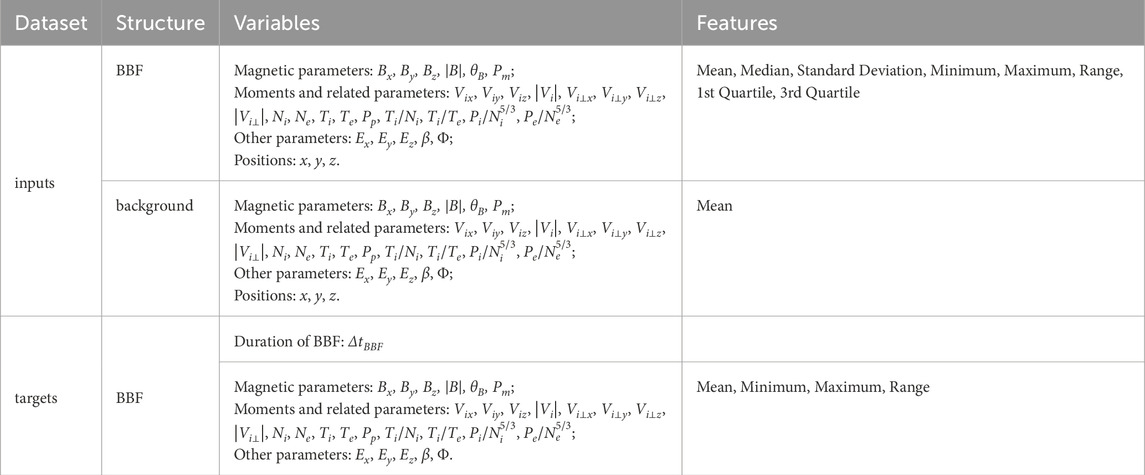
Table 1. Summary of machine learning model inputs and targets.
The targets include the BBF duration and a subset of physical variables considered predictable, each represented by four features: mean, maximum, minimum, and range during the BBF period. All predictions are conducted within this defined parameter space. To build and evaluate the model, a total of 3,207 BBF events are randomly split into training, validation, and test sets using a 7:1.5:1.5 ratio.
2.3 Selection of predictor variables
To address potential overfitting in the machine learning model and ensure that the predictions reflect meaningful physical connections, we aim to minimize the inclusion of irrelevant variables that could introduce noise or reduce the model’s predictive accuracy. This is achieved by analyzing the distributions of various variables during the background and BBF periods using kernel density estimation (KDE). By comparing the differences between these two time periods, we focus on identifying parameters that exhibit significant changes, as these are likely to have the potential for predictivity (i.e. relevant variables). The predictor variables in our model were selected based on their observed variability during the BBF period. Figure 2 illustrates the probability distribution of these parameters, with the central panel showing the overall probability density, and the left and top panels presenting the histogram distributions along each axis. The horizontal axis represents the mean value of
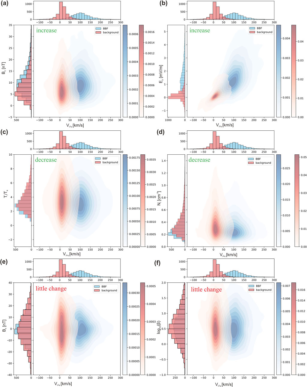
Figure 2. Comparison of the probability distributions of the average values of
Using KDE, we statistically analyze the distributions of mean values for the 28 physics parameters (excluding the three positional parameters) across all 3,207 BBFs during both the BBF and background periods. The analysis confirms that 19 parameters exhibit significant changes during the BBF period compared to the background period.
3 Methodology
Based on the fact that our sample size is low, we choose to use traditional machine learning methods. Traditional machine learning methods involve algorithms that learn patterns from data to make predictions or decisions, and these methods typically require manual feature extraction and selection, where domain expertise is crucial to identify relevant attributes from raw data (Bishop, 2006). Among these models, we evaluate three machine learning models: Support Vector Regression (SVR) (Smola and Schölkopf, 2004), Random Forest (Biau and Scornet, 2016), and XGBoost (Chen and Guestrin, 2016). After assessing their prediction performance on our test dataset, we select the XGBoost model as our prediction method. It builds decision trees sequentially, with each tree correcting the residuals (errors) of its predecessors. The trees are combined in an additive manner to enhance model performance, and regularization techniques are employed to prevent overfitting (Kakade et al., 2012). Specifically, we utilize a gradient boosting-based regression algorithm called “XGBRegressor” to model non-linear relationships in the data. Since we aim to predict multiple feature values of a specific BBF variable—including the mean, maximum, minimum, and range of the target parameter—we apply the MultiOutputRegressor (Pedregosa et al., 2011) wrapper to manage multiple output variables simultaneously, fitting a separate regressor for each target to ensure flexibility and efficiency.
After establishing the model, the subsequent step is to evaluate and compare its performance in predicting diverse target variables under various parameter combinations. In this study, we adopt a two-pronged approach for performance evaluation. We consider a Mean Absolute Percentage Error (MAPE) (Hyndman and Koehler, 2006) of 35% as the threshold for acceptable prediction. We empirically determined the 35% MAPE threshold through trial and error and manual inspection, balancing predictive accuracy with practical applicability. MAPE is advantageous as it represents errors in percentage terms, offering more intuitive insights compared to metrics like the Root Mean Squared Error (RMSE), which presents results in physical units. However, it should be noted that MAPE has its limitations. It can result in very large errors when the values are small. To provide a more comprehensive assessment, in the following results section, we will present tables for both MAPE and RMSE. This dual - metric presentation allows for a more thorough understanding of the model’s performance, especially considering that our parameters, such as velocity, can range over four orders of magnitude, from
4 Results
In our study, we examine diverse variable combinations and categorize the prediction tasks into two groups. These two groups are “Prediction Using Optimal Combination of Parameters” and “Cross - Instrument Prediction of Magnetic Field Parameters Using Plasma Moments.”
4.1 Prediction using optimal combination of parameters
In the first combination, referred to as the optimal combination of parameters, we utilize as many variables as possible to predict the target feature of a given variable. Our goal is to determine the upper and lower bounds of target variables during the BBF period. The target variable itself and any parameters that can be derived physically must be excluded from the input variables. For instance, when predicting the magnetic field, magnetic pressure cannot be included in the parameters. Through numerous attempts, we also discover that incorporating the mean value of the background of a target variable enhances the accuracy of its prediction, as shown in “Inputs – Additional variables during background” column in Table 2. Additionally, when predicting physical variables, adding positional parameters improves the MAPE value of prediction results by approximately one percentage point. The “Inputs – Variables during BBF and background” column in Table 2 presents all combinations of input physical parameters that are unrelated to the target variables and positional parameters.
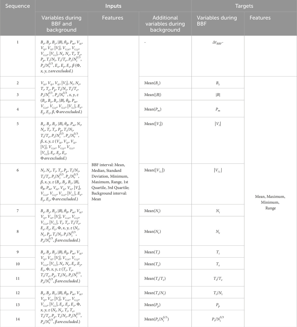
Table 2. Summary of using optimal combination of parameters to predict the mean, maximum, minimum, and range of BBF parameters.
This work focuses on predicting the previously selected 19 variables, which would likely change based on the probability distribution analysis. If the MAPE of the mean value is below 35% and at least two of the maximum, minimum, and range MAPE values in the test set are below 35%, we consider the prediction to be valid. This further eliminates six variables, including
The data structure used in the model is illustrated in Figure 3. This diagram illustrates how we organize the input and target features of sequence 5 of Table 2 in optimal combination. The input variables include magnetic components
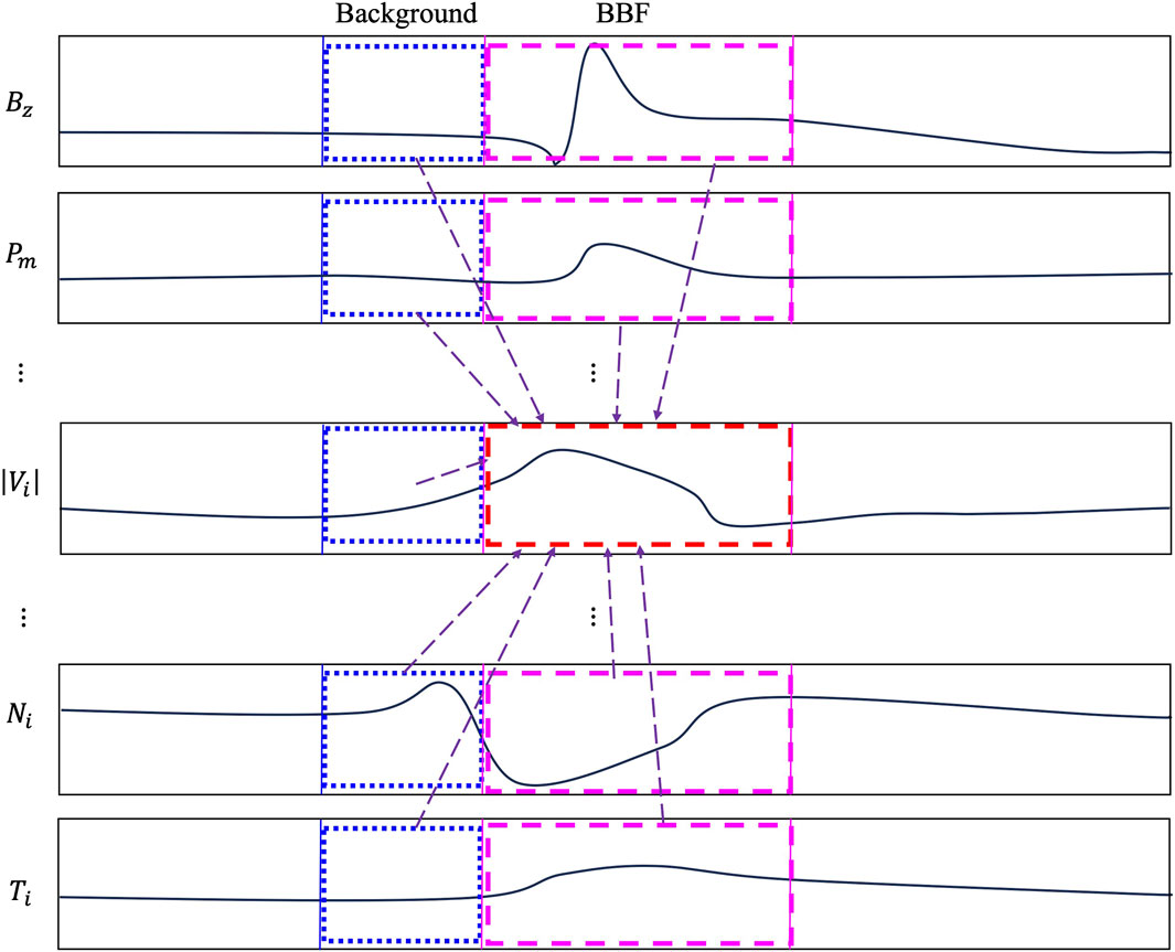
Figure 3. Input-output structure illustrated using
The statistical metric MAPE of the prediction results is showed in Table 3. The corresponding RMSE results are shown in Table 4.
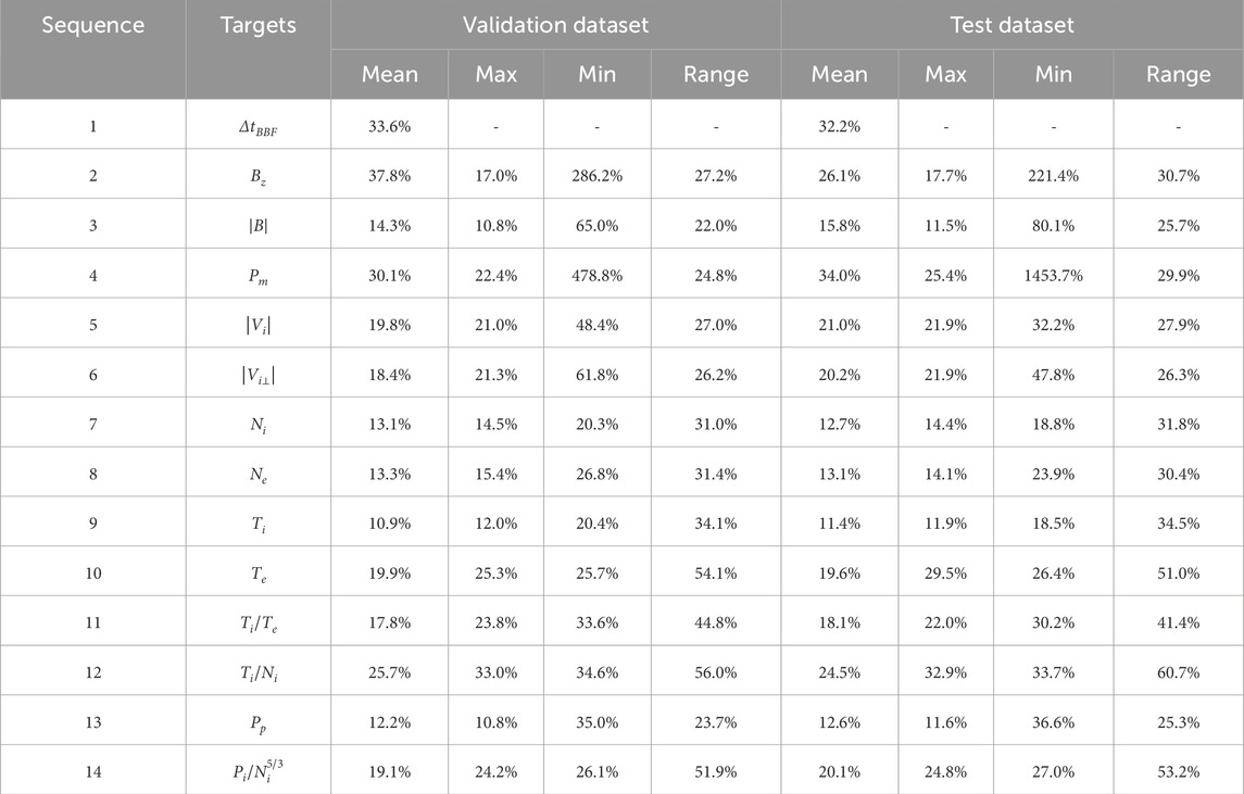
Table 3. MAPE of prediction results using the optimal combination on the validation dataset and test dataset. It should be noted that the result for ∆tBBF in the mean column represents ∆tBBF itself.
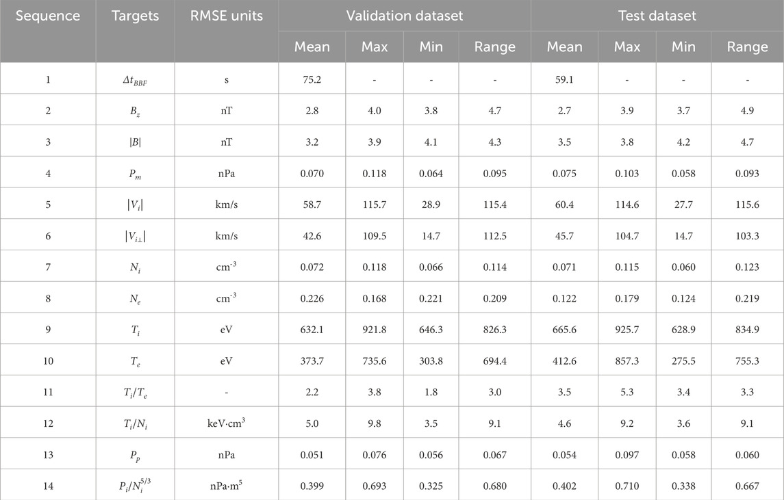
Table 4. RMSE of prediction results using the optimal combination on the validation dataset and test dataset. It should be noted that the result for ∆tBBF in the mean column represents ∆tBBF itself.
The comparison between the observed and predicted values for BBF duration in the test set is shown in Figure 4, while the comparisons for
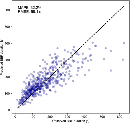
Figure 4. Comparison results between the observed and predicted values of BBF duration in the test set using optimal combination of parameters.
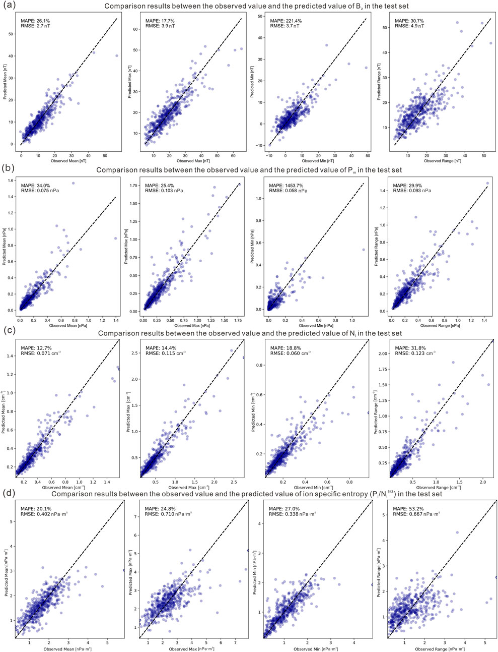
Figure 5. Comparison results between the observed values and the predicted values of (a)
Figure 6 illustrates how well the BBF duration and the corresponding maximum and minimum bounds of key physical parameters are predicted using our model. Panel (a) displays the main parameter
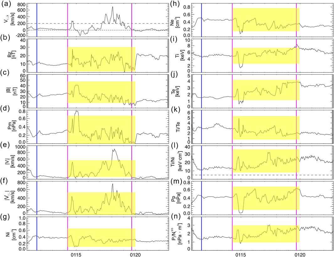
Figure 6. The BBF parameters observed by THD on 07 February 2008, between 01:10:49 and 01:22:49 at the position
After obtaining the prediction results, we further conducted a feature importance analysis to quantitatively assess the contribution of each input in the prediction process. We employed the leave-one-feature-out (LOFO) method, where one feature was removed at a time from the selected input parameter set. The XGBoost model was then retrained using the reduced feature set, and new prediction results on the test set were obtained.
To evaluate the impact of removing each feature, we calculated the differences in prediction performance compared to the baseline (i.e., predictions using the full input set). Specifically, we defined the performance drop as:
where
In most cases, both ΔMAPE and ΔRMSE are positive, indicating that removing the feature degrades prediction performance. However, for a small number of features, we observed negative ΔMAPE or ΔRMSE values, suggesting that excluding those features slightly improved performance, possibly due to noise or redundancy. We ranked all features based on ΔMAPE in descending order to identify the most influential ones in the prediction task.
Table 5 summarizes the analysis results. The first column lists each target parameter, while the second identifies the most influential feature for that target. The third and fourth columns report the corresponding ΔMAPE and ΔRMSE results, respectively. Notably, for 42 of the 52 target parameters, the background mean value of the same parameter emerges as the most significant factor, determined by its highest ΔMAPE. This finding underscores the critical role of background characteristics in predicting target parameter behavior during BBF events. For the remaining 10 targets, features observed during the BBF interval are the most influential inputs. However, no clear physical explanation exists for their primary influencing factors. Numerical simulations solving coupled physics equations could not isolate the effect of a single input while keeping others unchanged in self-consistent modeling. Additionally, we found that removing certain input variables improved prediction accuracy for some target parameters. These variables typically had small impact on the target prediction and were not listed in Table 5 as the most correlated inputs. All detailed results are available in the “feature_selection_result” folder on the referenced website.
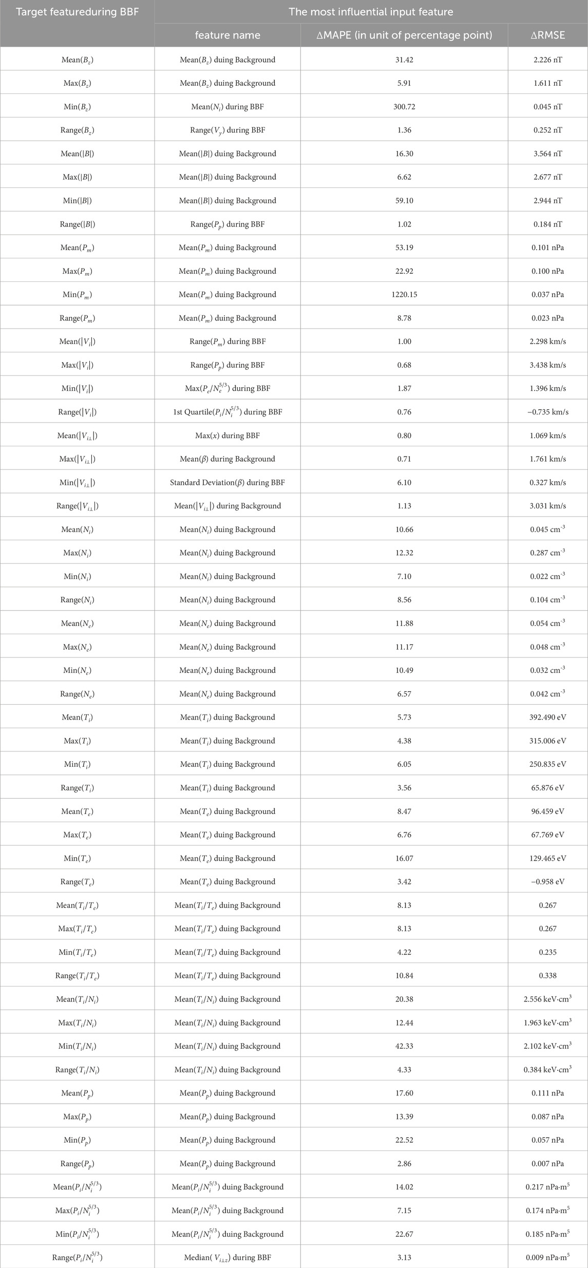
Table 5. Summary of the most influential input features for different target features.
4.2 Cross-instrument prediction of magnetic field parameters using plasma moments
We categorize the physical parameters into two main groups: plasma moment parameters and magnetic field parameters. These two categories originate from entirely different payloads. Among these, plasma moments—especially velocity—are critical for identifying BBFs, making their availability a prerequisite for our analysis. Therefore, in our cross-instrument prediction framework, we use plasma moment parameters, along with spacecraft location information, to predict magnetic field measurements.
The parameter combinations we used are summarized in Table 6, this table outlines the structure of input and target variables. The input variables are consistent across all sequences and include plasma moment data, as well as positional coordinates. These variables are statistically characterized by eight features within the BBF interval (mean, median, standard deviation, minimum, maximum, range, first quartile, and third quartile) and one feature (mean) within the background interval. Each sequence targets a different magnetic parameter during the BBF interval.
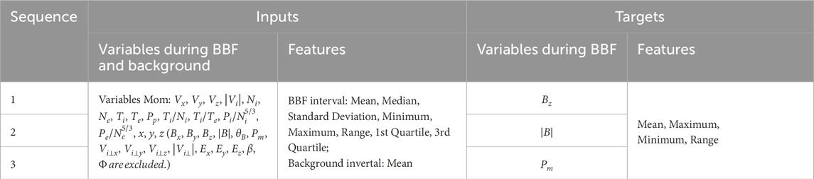
Table 6. Summary of cross-instrument prediction of magnetic field using plasma moments.
An example of the data structure for the cross-instrument prediction parameter combination is shown in Figure 7. This figure corresponds to the inputs-outputs structure used for predicting
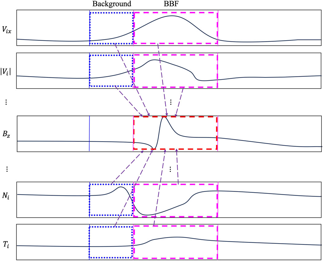
Figure 7. Similar to Figure 3. Input-output structure of cross-instrument prediction of
Through testing, we find that the predictions for
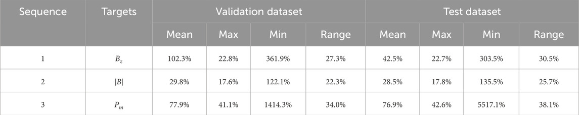
Table 7. MAPE of cross-instrument prediction results of magnetic field using plasma moments without additional background inputs.
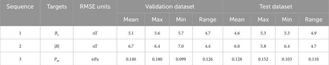
Table 8. RMSE of cross-instrument prediction results of magnetic field using plasma moments without addictional background inputs.
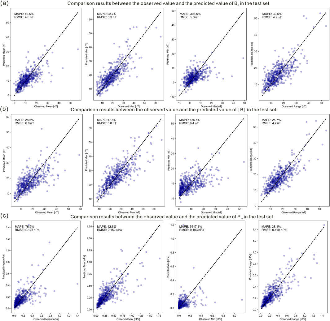
Figure 8. Similar to Figure 5. Comparison results between the observed and predicted values of magnetic field targets (a)
An example of predicted ranges along with the measurements is shown in Figure 9. The yellow shadow box indicates that we can predict
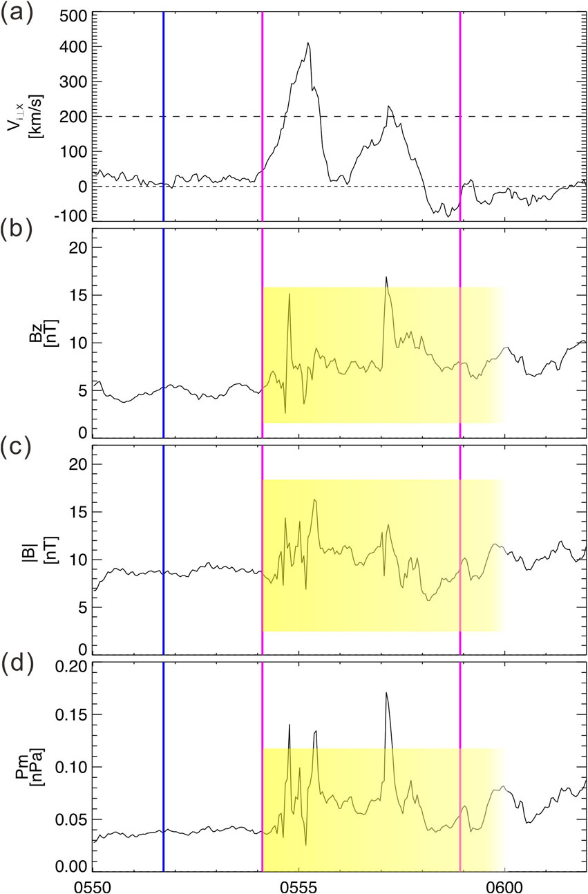
Figure 9. Similar to Figure 6. Predicted ranges using cross-instrument prediction of magnetic field measurements using plasma moments without additional background variables as inputs. This event was observed by THE on 07 March 2008, between 05:49:59 and 06:01:59 at the position
While cross-instrument prediction without additional background data remains challenging, adding observed background mean values as additional inputs can significantly improve performance. In order to illustrate the importance of using accurate background values as ML model inputs in the cross-instrument prediction, we add the mean values of the background periods calculated using actual observations of the background. The MAPE of prediction results are below the 35% MAPE threshold which are shown in Supplementary Table S3, and the time series with predicted bounds for the same event are shown in Supplementary Figure S3. This highlights the importance of background context in achieving robust predictions. The MAPE of these two different additional background values as inputs, are compared in Figure 10. Each bar in the figure represents the average of the three MAPE values (the mean, maximum, and range) on the test set. The error bars represent one standard deviation of the MAPE of the predictions for these three features. It clearly demonstrates that using the target variable’s mean value calculated from actual measurements during the background period can significantly enhance prediction accuracy. For example, for the predicted mean, maximum, and range values during the BBF period in the test dataset, we can see that when using observed background values as additional inputs, the average MAPE results for
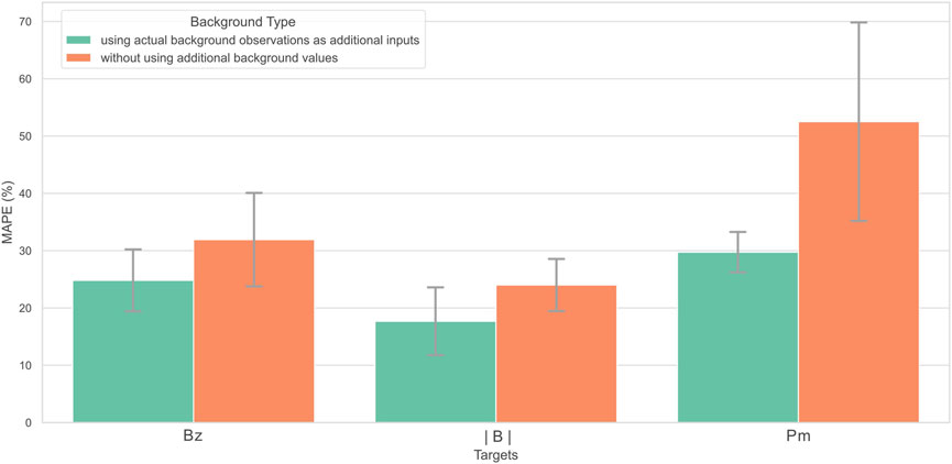
Figure 10. Effect of background information on BBF prediction error. The horizontal axis represents the target variables:
5 Discussion and summary
Our initial objective was to predict the entire time series of target parameters throughout the BBF period. However, this idea proved impractical due to three primary challenges. First, data limitations significantly constrained our analysis. Despite utilizing all available THEMIS BBF observations, the scarcity of space weather events resulted in only 3,207 BBFs, which was an insufficient sample size for robust time series predictions. Second, the complexity and variability of BBF parameter fluctuations posed a major challenge. BBFs often occurred in rapid succession, making their identification difficult even for experienced scientists. This irregularity made it challenging for machine learning models to detect consistent patterns necessary for accurate time-series forecasting. Finally, the presence of excessive microscale variations within BBF time series further complicated prediction efforts. Even after applying strict selection criteria, the inherent variability in parameters—due to background fluctuations and observational noise—remained significant.
To address these challenges, we adopted a feature-based prediction approach, leveraging all available BBF data from 2007 to 2023. Instead of attempting full time-series reconstruction, we focused on identifying predictable features of various parameters. By analyzing the differences between BBF and background periods, we identified parameters that have distinct changing patterns and thus allow for target prediction. We tested different parameter combinations and categorized them into two primary strategies: (1) optimal combinations, where we used as many parameters as possible to maximize prediction accuracy, and (2) cross-instrument prediction, where we leveraged plasma moments parameters to predict magnetic field parameters.
With the optimal combination, we were able to predict BBF duration with a mean absolute percentage error (MAPE) below 35%. Furthermore, we achieved good accuracy for predictions of the maximum and minimum ranges of thirteen key physical parameters, including
For cross-instrument predictions, the results indicate that including accurate target background as an additional input significantly improves the prediction accuracy. By leveraging improved background estimates, we can enhance the reliability of predictions not only for individual BBF parameters but also for broader space weather applications.
Our findings have practical implications for situations where satellites may lack certain payloads or where instrument failures occur. By supplementing missing BBF parameters, our model enhances data utility for space weather research. Expanding the dataset with more comprehensive observations is crucial for improving prediction accuracy. Moving forward, we anticipate that using larger and more diverse datasets (for example, augmenting Geotail, Cluster, and MMS observations) will substantially enhance the model’s performance, bringing us closer to a more precise characterization of BBF dynamics.
Data availability statement
The original contributions presented in the study are included in the article/Supplementary Material, further inquiries can be directed to the corresponding author.
Author contributions
XF: Conceptualization, Data curation, Formal Analysis, Investigation, Methodology, Software, Validation, Visualization, Writing – original draft, Writing – review and editing. JY: Conceptualization, Data curation, Formal Analysis, Funding acquisition, Investigation, Methodology, Project administration, Resources, Software, Supervision, Validation, Visualization, Writing – original draft, Writing – review and editing. JB: Writing – review and editing, Conceptualization, Formal Analysis, Methodology, Supervision, Validation. C-PW: Formal Analysis, Methodology, Validation, Visualization, Writing – review and editing. JL: Formal Analysis, Methodology, Validation, Visualization, Writing – review and editing.
Funding
The author(s) declare that financial support was received for the research and/or publication of this article. This work was supported by Grant 42174197 of the National Natural Science Foundation of China (NSFC), Shenzhen Science and Technology Program (Grant JCYJ20220530113402004).
Conflict of interest
The authors declare that the research was conducted in the absence of any commercial or financial relationships that could be construed as a potential conflict of interest.
Generative AI statement
The authors declare that Gen AI was used in the creation of this manuscript. The author verify and take full responsibility for the use of generative AI in the preparation of this manuscript. Generative AI was used to assist with language editing. The authors reviewed and critically revised the AI-generated content to ensure accuracy, originality, and adherence to academic standards.
Publisher’s note
All claims expressed in this article are solely those of the authors and do not necessarily represent those of their affiliated organizations, or those of the publisher, the editors and the reviewers. Any product that may be evaluated in this article, or claim that may be made by its manufacturer, is not guaranteed or endorsed by the publisher.
Supplementary material
The Supplementary Material for this article can be found online at: https://www.frontiersin.org/articles/10.3389/fspas.2025.1582607/full#supplementary-material
References
Angelopoulos, V. (2008). The THEMIS mission. Space Sci. Rev. 141 (1–4), 5–34. doi:10.1007/s11214-008-9336-1
Angelopoulos, V., Baumjohann, W., Kennel, C. F., Coroniti, F. V., Kivelson, M. G., Pellat, R., et al. (1992). Bursty bulk flows in the inner central plasma sheet. J. Geophys. Res. 97 (A4), 4027–4039. doi:10.1029/91JA02701
Angelopoulos, V., Kennel, C. F., Coroniti, F. V., Pellat, R., Kivelson, M. G., Walker, R. J., et al. (1994). Statistical characteristics of bursty bulk flow events. J. Geophys. Res. 99 (A11), 21257–21280. doi:10.1029/94JA01263
Ashour-Abdalla, M., El-Alaoui, M., Goldstein, M. L., Zhou, M., Schriver, D., Richard, R., et al. (2011). Observations and simulations of non-local acceleration of electrons in magnetotail magnetic reconnection events. Nat. Phys. 7 (4), 360–365. doi:10.1038/nphys1903
Auster, H. U., Glassmeier, K. H., Magnes, W., Aydogar, O., Baumjohann, W., Constantinescu, D., et al. (2008). The THEMIS fluxgate magnetometer. Space Sci. Rev. 141 (1–4), 235–264. doi:10.1007/s11214-008-9365-9
Biau, G., and Scornet, E. (2016). A random forest guided tour. TEST 25 (2), 197–227. doi:10.1007/s11749-016-0481-7
Birn, J., Nakamura, R., Panov, E. V., and Hesse, M. (2011). Bursty bulk flows and dipolarization in MHD simulations of magnetotail reconnection: BURSTY FLOWS AND DIPOLARIZATIONS. J. Geophys. Res. Space Phys. 116 (A1). doi:10.1029/2010JA016083
Birn, J., Raeder, J., Wang, Y. L., Wolf, R. A., and Hesse, M. (2004). On the propagation of bubbles in the geomagnetic tail. Ann. Geophys. 22 (5), 1773–1786. doi:10.5194/angeo-22-1773-2004
Bortnik, J., Chu, X., Ma, Q., Li, W., Zhang, X., Thorne, R. M., et al. (2018). “Artificial neural networks for determining magnetospheric conditions,” in Machine learning techniques for space weather (Elsevier), 279–300. doi:10.1016/B978-0-12-811788-0.00011-1
Camporeale, E. (2019). The challenge of machine learning in space weather: nowcasting and forecasting. Space weather. 17 (8), 1166–1207. doi:10.1029/2018SW002061
Cao, J., Ma, Y., Parks, G., Reme, H., Dandouras, I., and Zhang, T. (2013). Kinetic analysis of the energy transport of bursty bulk flows in the plasma sheet. J. Geophys. Res. Space Phys. 118 (1), 313–320. doi:10.1029/2012JA018351
Chen, C. X., and Wolf, R. A. (1999). Theory of thin-filament motion in Earth’s magnetotail and its application to bursty bulk flows. J. Geophys. Res. Space Phys. 104 (A7), 14613–14626. doi:10.1029/1999JA900005
Chen, T., and Guestrin, C. (2016). “XGBoost: a scalable tree boosting system,” in Proceedings of the 22nd ACM SIGKDD international conference on knowledge discovery and data mining (San Francisco California USA: ACM), 785–794. doi:10.1145/2939672.2939785
Chen, Y.-C. (2017). A tutorial on kernel density estimation and recent advances. Biostat. & Epidemiol. 1 (1), 161–187. doi:10.1080/24709360.2017.1396742
Feng, X., and Yang, J. (2023). Plasma-sheet bubble identification using multivariate time series classification. J. Geophys. Res. Space Phys. 128 (10), e2023JA031469. doi:10.1029/2023JA031469
Forsyth, C., Lester, M., Cowley, S. W. H., Dandouras, I., Fazakerley, A. N., Fear, R. C., et al. (2008). Observed tail current systems associated with bursty bulk flows and auroral streamers during a period of multiple substorms. Ann. Geophys. 26 (1), 167–184. doi:10.5194/angeo-26-167-2008
Grocott, A., Yeoman, T. K., Nakamura, R., Cowley, S. W. H., Frey, H. U., Rème, H., et al. (2004). Multi-instrument observations of the ionospheric counterpart of a bursty bulk flow in the near-Earth plasma sheet. Ann. Geophys. 22 (4), 1061–1075. doi:10.5194/angeo-22-1061-2004
Henderson, M. G., Reeves, G. D., and Murphree, J. S. (1998). Are north-south aligned auroral structures an ionospheric manifestation of bursty bulk flows? Geophys. Res. Lett. 25 (19), 3737–3740. doi:10.1029/98GL02692
Hu, B., Wolf, R. A., Toffoletto, F. R., Yang, J., and Raeder, J. (2011). Consequences of violation of frozen-in-flux: evidence from OpenGGCM simulations: BRIEF REPORT. J. Geophys. Res. Space Phys. 116 (A6). doi:10.1029/2011JA016667
Hyndman, R. J., and Koehler, A. B. (2006). Another look at measures of forecast accuracy. Int. J. Forecast. 22 (4), 679–688. doi:10.1016/j.ijforecast.2006.03.001
Kakade, S. M., Shalev-Shwartz, S., and Tewari, A. (2012). Regularization techniques for learning with. Matrices 13 (1), 1865–1890. doi:10.5555/2503308.2343703
Liu, J., Angelopoulos, V., Runov, A., and Zhou, X.-Z. (2013). On the current sheets surrounding dipolarizing flux bundles in the magnetotail: the case for wedgelets. J. Geophys. Res. Space Phys. 118 (5), 2000–2020. doi:10.1002/jgra.50092
McFadden, J. P., Carlson, C. W., Larson, D., Ludlam, M., Abiad, R., Elliott, B., et al. (2008). The THEMIS ESA plasma instrument and in-flight calibration. Space Sci. Rev. 141 (1–4), 277–302. doi:10.1007/s11214-008-9440-2
Merkin, V. G., Panov, E. V., Sorathia, K. A., and Ukhorskiy, A. Y. (2019). Contribution of bursty bulk flows to the global dipolarization of the magnetotail during an isolated substorm. J. Geophys. Res. Space Phys. 124 (11), 8647–8668. doi:10.1029/2019JA026872
Nakamura, R., Amm, O., Laakso, H., Draper, N. C., Lester, M., Grocott, A., et al. (2005). Localized fast flow disturbance observed in the plasma sheet and in the ionosphere. Ann. Geophys. 23 (2), 553–566. doi:10.5194/angeo-23-553-2005
Nakamura, R., Baumjohann, W., Klecker, B., Bogdanova, Y., Balogh, A., Rème, H., et al. (2002). Motion of the dipolarization front during a flow burst event observed by Cluster. Geophys. Res. Lett. 29 (20). doi:10.1029/2002GL015763
Nakamura, R., Baumjohann, W., Schödel, R., Brittnacher, M., Sergeev, V. A., Kubyshkina, M., et al. (2001). Earthward flow bursts, auroral streamers, and small expansions. J. Geophys. Res. Space Phys. 106 (A6), 10791–10802. doi:10.1029/2000JA000306
Nishimura, Y., Lyons, L., Zou, S., Angelopoulos, V., and Mende, S. (2010). Substorm triggering by new plasma intrusion: THEMIS all-sky imager observations. J. Geophys. Res. Space Phys. 115 (A7), 2009JA015166. doi:10.1029/2009JA015166
Ohtani, S., Singer, H. J., and Mukai, T. (2006). Effects of the fast plasma sheet flow on the geosynchronous magnetic configuration: Geotail and GOES coordinated study. J. Geophys. Res. Space Phys. 111 (A1), 2005JA011383. doi:10.1029/2005JA011383
Ohtani, S.-ichi, Shay, M. A., and Mukai, T. (2004). Temporal structure of the fast convective flow in the plasma sheet: comparison between observations and two-fluid simulations. J. Geophys. Res. 109 (A3), A03210. doi:10.1029/2003JA010002
Pedregosa, F., Varoquaux, G., Gramfort, A., Michel, V., Thirion, B., Grisel, O., et al. (2011). Scikit-learn: machine learning in Python. Mach. Learn. PYTHON. doi:10.5555/1953048.2078195
Pontius, D. H., and Wolf, R. A. (1990). Transient flux tubes in the terrestrial magnetosphere. Geophys. Res. Lett. 17 (1), 49–52. doi:10.1029/GL017i001p00049
Runov, A., Angelopoulos, V., Artemyev, A., Birn, J., Pritchett, P. L., and Zhou, X.-Z. (2017). Characteristics of ion distribution functions in dipolarizing flux bundles: event studies. J. Geophys. Res. Space Phys. 122 (6), 5965–5978. doi:10.1002/2017JA024010
Runov, A., Angelopoulos, V., Gabrielse, C., Liu, J., Turner, D. L., and Zhou, X.-Z. (2015). Average thermodynamic and spectral properties of plasma in and around dipolarizing flux bundles. J. Geophys. Res. Space Phys. 120 (6), 4369–4383. doi:10.1002/2015JA021166
Sergeev, V. A., Chernyaev, I. A., Dubyagin, S. V., Miyashita, Y., Angelopoulos, V., Boakes, P. D., et al. (2012). Energetic particle injections to geostationary orbit: relationship to flow bursts and magnetospheric state. J. Geophys. Res. Space Phys. 117 (A10), 2012JA017773. doi:10.1029/2012JA017773
Shi, Y., Zesta, E., Lyons, L. R., Yang, J., Boudouridis, A., Ge, Y. S., et al. (2012). Two-dimensional ionospheric flow pattern associated with auroral streamers. J. Geophys. Res. Space Phys. 117 (A2), 2011JA017110. doi:10.1029/2011JA017110
Sitnov, M., Birn, J., Ferdousi, B., Gordeev, E., Khotyaintsev, Y., Merkin, V., et al. (2019). Explosive magnetotail activity. Space Sci. Rev. 215 (4), 31. doi:10.1007/s11214-019-0599-5
Sitnov, M. I., Guzdar, P. N., and Swisdak, M. (2005). On the formation of a plasma bubble. Geophys. Res. Lett. 32 (16), 2005GL023585. doi:10.1029/2005GL023585
Smola, A. J., and Schölkopf, B. (2004). A tutorial on support vector regression. Statistics Comput. 14 (3), 199–222. doi:10.1023/B:STCO.0000035301.49549.88
Wolf, R. A., Wan, Y., Xing, X., Zhang, J.-C., and Sazykin, S. (2009). Entropy and plasma sheet transport. J. Geophys. Res. Space Phys. 114 (A9), 2009JA014044. doi:10.1029/2009JA014044
Yang, J., Toffoletto, F. R., Wolf, R. A., and Sazykin, S. (2011). RCM-E simulation of ion acceleration during an idealized plasma sheet bubble injection: BUBBLE INJECTION. J. Geophys. Res. Space Phys. 116 (A5). doi:10.1029/2010JA016346
Keywords: parameter prediction, MultiOutputRegressor, bursty bulk flows, cross-instrument, minimum, maximum, range
Citation: Feng X, Yang J, Bortnik J, Wang C-P and Liu J (2025) Predicting characteristics of bursty bulk flows in Earth’s plasma sheet using machine learning techniques. Front. Astron. Space Sci. 12:1582607. doi: 10.3389/fspas.2025.1582607
Received: 24 February 2025; Accepted: 12 May 2025;
Published: 03 June 2025.
Edited by:
Weichao Tu, West Virginia University, United StatesReviewed by:
Andrew Smith, Northumbria University, United KingdomYue Chen, Los Alamos National Laboratory (DOE), United States
Copyright © 2025 Feng, Yang, Bortnik, Wang and Liu. This is an open-access article distributed under the terms of the Creative Commons Attribution License (CC BY). The use, distribution or reproduction in other forums is permitted, provided the original author(s) and the copyright owner(s) are credited and that the original publication in this journal is cited, in accordance with accepted academic practice. No use, distribution or reproduction is permitted which does not comply with these terms.
*Correspondence: Xuedong Feng, ZmVuZ3hkMjAyMUBtYWlsLnN1c3RlY2guZWR1LmNu