 Vicki Toy-Edens
 Wenli Mo
 Robert C. Allen
 Sarah K. Vines
 Savvas Raptis
- 1Johns Hopkins University Applied Physics Laboratory, Laurel, MD, United States
- 2Southwest Research Institute, San Antonio, TX, United States
Our methodology demonstrates a proof of concept of the applicability of transfer learning for heliophysics, a machine learning technique where knowledge learned from one task is reused to perform a similar unsupervised learning task with additional fine tuning. We applied an unsupervised clustering algorithm, initially trained on data from the Magnetospheric Multiscale (MMS) mission at Earth, to MErcury Surface, Space ENvironment, GEochemistry, and Ranging (MESSENGER) observationsat Mercury to identify three distinct plasma regions: magnetosphere, magnetosheath, and solar wind. While our method requires modifications to the model from post-cleaning rules due to instrument effects, it allows for rapid classification using just a few examples to generate post-cleaning rules. Since there is no ground truth or standardized validation set to compare with, we compare our model’s result with published magnetopause and bow shock lists and find that the clustering algorithm is agreement with 67% of bow shock crossings and 74% of magnetopause crossings. These findings highlight the potential use of clustering algorithms across multiple planetary environments.
1 Introduction
Distinguishing between different plasma regimes and systems (e.g., solar wind, magnetosheath, and magnetosphere) is important for understanding the local dynamics and driving conditions of solar wind-magnetosphere interactions. For identifying distinct plasma regions at Earth, Toy-Edens et al. (2024b) (hereafter T24) created an automated in-situ plasma region classifier trained on 8 years of dayside Magnetospheric Multiscale (MMS) mission data (for more details about MMS, see Burch et al., 2015). The T24 model is based on an unsupervised Gaussian Mixture Model clustering method that is coupled with a post-cleaning process. This tunable approach enables automated labeling for all dayside plasma regimes as well as identifying each transition between plasma regimes (e.g., magnetopause and bow shock). We clarify here that this model is automated in the sense that there is a pre-defined standardized set of conditions that lead to a particular label that does not require manual review of each epoch. Combined with the straightforward nature of the features going into the model (simple normalized sums and ratios created from ion spectra and magnetic field measurements), the resulting model is lightweight and extensible.
In this work, we test the extensibility of the T24 model to evaluate whether the model, trained on Earth’s magnetospheric environment, can be extended to other planetary magnetospheres with different available instrumentation and datasets. We are calling this process “unsupervised transfer learning”. Transfer learning is a machine learning technique where knowledge learned from one task is reused to perform a similar task; in this case, knowledge gained from data-rich Earth observations is applied to other, less extensive planetary datasets. This usually requires fine tuning the model on the relevant and desired dataset. While this approach does not alleviate the need to tune the model, it requires substantially less training data and effort than training a brand new model from scratch. More often than not, this technique implies the use of neural networks, but here we invoke the more general definition and denote the difference by specifying unsupervised learning, where there are no ground truth labels, opposed to one that includes pre-existing labels. This problem is an unsupervised learning problem as there are no ground truth labels.
Previous works have built specialized models based on the characteristics of each planet and/or specific dataset (e.g., James et al., 2020). However, the ability to train particular models this way can be limited by the volume of data already collected. These models cannot be trained until a critical level of data has been amassed, which usually means late in the lifetime of a mission. For data sparse environments, like at planetary magnetospheres beyond Earth, it is more advantageous to instead train, test, and refine models on existing large and varied datasets and then perform precision tuning for different environments with data from a desired mission. While one could manually select boundaries in these data-sparse environments, an automated method with minimal adjustments would allow for consistent identification of plasma regimes across multiple planetary magnetospheric environments and quick, initial determinations of in-situ regions and events of interest. A broadly applicable automated method may also aid in reanalysis of historical datasets or in statistical studies spanning multiple missions at the same system in a more unified approach.
Therefore, there is extreme value in using an extensible model across multiple planetary bodies to create an automated and standardized dataset with the same underlying methodology. A standard method also allows for studies of how transitions are similar or different across different planetary magnetospheric systems. Beyond applying the model across multiple magnetospheric systems, this also demonstrates the feasibility of applying such an algorithm to a wide range of datasets, with their own limitations, advantages, and considerations, to reach a mission-agnostic boundary determination scheme.
In particular, this study aims to apply the T24 model to the magnetosphere of Mercury as a proof of concept of the applicability of the T24 model. Mercury is a good first test case to extend the T24 model because, similar to Earth, it is a solar wind-driven (i.e., Dungey cycle-dominant) magnetosphere (Dungey, 1961; Slavin et al., 2021) rather than an internally-driven (i.e., Vasyliunas-dominant) system like the outer planets (Vasyliunas, 1983). However, while the magnetospheres of Earth and Mercury are both solar wind-driven, Mercury’s magnetosphere has important differences from Earth’s due to the nature of Mercury’s magnetic field, large-scale current closure, and the lack of an extensive atmosphere. More specifically, Mercury’s magnetosphere is smaller and experiences stronger solar wind dynamic pressures because of the location of Mercury at 0.307–0.467 AU, allowing for much faster timescales for dynamics such as flux transfer events and sub-storms (see review by Sun et al., 2022). We will apply the T24 model to MErcury Surface, Space Environment, GEochemistry, and Ranging (MESSENGER, Solomon et al., 2007) dayside data and evaluate the effectiveness and ease of adapting an Earth-based model to Mercury. We limit our evaluation to Mercury’s dayside because the original T24 model was only trained and evaluated on Earth’s dayside. The resulting plasma region labels, identified transitions, and region identification model may prove useful for the upcoming observations of Mercury from BepiColombo (Benkhoff et al., 2021).
2 Materials and methods
2.1 Data
MESSENGER launched on August 2, 2004 and, after extensive flybys, entered into a highly elliptical, polar orbit around Mercury in March 2011. MESSENGER remained in its polar orbit until the mission ended in April 2015. In this study, we use data from the dayside (
For low-energy plasma data, we utilize the Energetic Particle and Plasma Spectrometer (EPPS) Fast Imaging Plasma Spectrometer (FIPS; Andrews et al., 2007) Level 3 calibrated scan data. The FIPS scan data covers the energy/charge range of
We also use the magnetometer (MAG; Anderson et al., 2007) Level 3 calibrated data in MSO coordinates for the magnetic field measurements reported at 0.05 s resolution. We down-sample this data to a 1-min resolution to match the resampled FIPS resolution by taking the mean of the resampled data in 1-min increments. We note that we maintain the full magnetometer time resolution for visualization purposes only.
2.2 MMS model
T24 trained and applied an unsupervised clustering model (Gaussian Mixture Model) on generalized features generated from MMS dayside (X norm_Bt, ratio_max_width, and ratio_high_low) that are used to cluster plasma regions are ratios of observable quantities. The generated features are useful for identifying patterns that are commonly used to manually identify plasma regions. In particular, these features focus on identifying narrow versus wide ion spectra peaks, high versus low energy excesses in ion spectra, and high versus low magnetic field values. norm_Bt is the total magnetic field normalized to 50 nT. The choice of 50 nT for normalization is somewhat arbitrary, though was found to be generally useful for distinguishing larger, magnetospheric magnetic field strengths from the typically very small interplanetary magnetic field (IMF) strength. The ratio_max_width and ratio_high_low quantities are based on spectra of the bulk ion populations: ratio_max_width is the width of the largest peak in energy bins normalized to the number of available energy bins and ratio_high_low is the ratio of the mean of the intensity for energies
Due to the general nature of the features and the data requirements of the T24 model, we can apply this extensible model to other planetary systems without having to retrain the model. Essentially, this makes use of a data-rich environment (the model utilizes 66,498 h of Earth observations) and applies it to more data-starved observations. We extend the T24 model to dayside orbit observations of MESSENGER data with some minor feature alterations (Section 2.3) and post-cleaning (Section 2.4) to identify three plasma regions around Mercury: magnetosphere, magnetosheath, and solar wind. Figure 1 shows an example of the T24 clustering algorithm applied to MMS and MESSENGER data for similar plasma conditions. We note that the MMS clustering label around 11:00 UTC has been modified from the ion foreshock label (a subset of the solar wind population) to the more general solar wind label for a more direct comparison to MESSENGER data. The clustering contours in T24 (their Figure 3) show that the solar wind and ion foreshock are closely spaced clusters in each slice of feature space, which is expected given that the ion foreshock is by definition a population within the solar wind. Given that the MESSENGER and MMS datasets have different temporal and energy resolutions, and a goal of the region identification is to identify boundary transitions, we do not attempt to distinguish ion foreshock separately from the more “pristine” solar wind with the MESSENGER data.
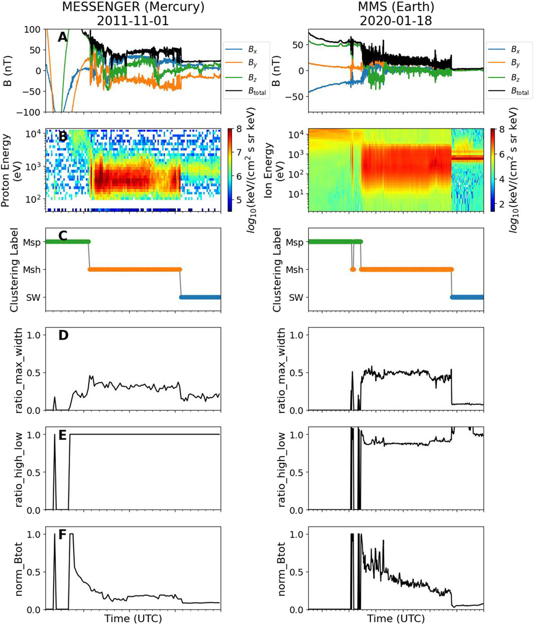
Figure 1. A side-by-side comparison of MESSENGER data from 2011 November 01 (left) and MMS data from 2020 January 18 (right). Both show the magnetic field (A) and proton or total ion fluxes (B) alongside the unsupervised clustering labels (C) and values for each generated feature (D–F). These two time periods show a similar trajectory of the spacecraft passing through magnetosphere (Msp) into magnetosheath (Msh), and eventually into solar wind (SW) plasma. The T24 clustering algorithm utilizes generalized features in the magnetic field and proton/total ion spectral properties for each region (e.g., wide peak in proton/ion spectra in the magnetosheath versus a narrow peak in the solar wind) that can be applied to different planets and missions.
2.3 Feature engineering
While MESSENGER has both an ion spectrometer and magnetometer like MMS, FIPS does not have full-sky coverage and the spacecraft is three-axis stabilized. Combining this with the fact that MESSENGER’s thermal shield design also obstructs instrument measurements in the solar direction (Gershman et al., 2012), FIPS observations often miss the narrow solar wind beam, unlike the MMS ion instruments. Generally, and useful for T24, the narrow beam is a very distinct signature that the spacecraft was in the solar wind. Likewise, the lack of full-sky coverage also may mean that the linear increase of flux with energy in ion spectra associated with the magnetospheric regions in T24 is not always captured by MESSENGER data. Finally, MESSENGER observations do not often see the elevated high-energy signature associated with the ion foreshock. This ultimately means that while we can use the existing clustering model, we must add additional rules in post-processing and alter the feature generation to account for these observational differences.
The T24 model is based upon generalized ratios of MMS ion spectra and total magnetic field, however, different planetary magnetosphere, mission profile, and instrument effects have to be taken into account for feature engineering. Nevertheless, with minimal visual inspection of a handful of examples, we can recreate the same patterns that the T24 clustering model relies on (i.e., wide versus narrow proton/ion energy peaks or high versus low total magnetic field). This is possible because the plasma regimes have distinct characteristics that can be quickly identified. For example, solar wind plasma is usually characterized by a narrow proton/ion beam at around 1 keV in energy, which is quite distinct from the heated (and so broad) ion fluxes at 100s eV to 1’s keV in the magnetosheath.
ratio_max_width (shown in Figure 1D) is calculated similarly to the T24 method where the width in energy bins of the most prominent peak in ion spectra identified by a peak-finding algorithm is normalized by the number of possible energy bins. MESSENGER FIPS data is more coarse in energy than MMS FPI-DIS, so we can utilize the full width of the most prominent peak. We also increase the required minimum peak intensity from 1 to 1.5 to perform a peak fitting due to the difference in ion spectra intensities between the magnetospheres.
The ratio_high_low (shown in Figure 1E) parameter primarily helps distinguish between ion foreshock and solar wind. As we do not attempt to separate out these populations in this study, we set this feature to 1 if a peak in the ion spectra is found. Otherwise we set this feature to 0, akin to the magnetosphere pseudo-feature (an indirect feature that alters other features but is not included in a clustering model) described in T24.
norm_Bt (shown in Figure 1F) follows the same definition as done for the MMS norm_Bt feature, except that instead of normalizing the magnetic field to 50 nT, we instead use 150 nT for Mercury due to the difference in magnetic field strength in each planet’s magnetosphere near dayside the magnetopause. We note that this normalization value may at times lead to an overly conservative feature definition, where identification of magnetopause transitions at larger radial distances may be impacted.
As done in T24, we utilize a pseudo-feature to characterize the magnetospheric plasma when a peak in the proton spectra is not detected. This pseudo-feature sets the other three features (norm_Bt, ratio_max_width, and ratio_high_low) to zero to place this type of signature in a distinct location in feature space. We note that while this worked well for MMS, it creates a need for additional post-processing features for use with MESSENGER: spectra_counts and high_intensity_peak. Often there are 1-min time periods with no or few proton counts. In order to avoid incorrectly classifying these data points (typically as magnetosphere, as this means there is no proton spectra peak), we have a feature to identify these times (spectra_counts) which is the ratio of the number of non-zero proton energy bins over the total number of proton energy bins. These are labeled as an “unknown” plasma region out of an abundance of caution to not mislabel a region due to lack of proton counts. As mentioned before, there is often missing information due to the lack of full-sky coverage in the proton spectra that may cause magnetosheath plasma to resemble magnetospheric populations when the core of the proton distributions are not within the instrument field-of-view. In order to address this we do an additional peak fitting that enforces a higher minimum peak intensity threshold of 2.25 instead of 1.5 and generates a Boolean feature (high_intensity_peak) that solely indicates if a peak was found with the higher minimum peak intensity threshold. The use of these two additional features is described in Section 2.4.
2.4 Post-processing and cleaning
We use the adapted feature generation described in Section 2.3 and apply the T24 model to the features to generate classification labels at 1-min resolution. T24 describes additional post-processing steps used to clean up the clustering identifications. We perform a similar process using the rules outlined in Table 1. The raw dataset has 439,329 magnetosphere, 302,739 solar wind, and 278,015 magnetosheath 1-min observations. We first identify regions with specific classification labels (“Original” label in Table 1) and then find where those classifications also have the same conditions as the “relabel” rules to create a new, “cleaned” label (the “Resultant Label” in Table 1). We note that our dataset maintains the original raw clustering labels alongside any “cleaned” labels so that researchers may elect to apply their own post-cleaning rules.
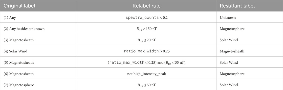
Table 1. Relabeling rules.
We largely relied on the total magnetic field,
The remainder of the relabeling rules alter 10% (103,014) of the labels from their initial clustering labels. These rules were determined from visual inspection of approximately 50 random samples. Before applying the rules broadly, we first examined the distributions of the rules and visually inspected 10 randomly sampled days from a larger collection of dates with intervals that meet the relabel rule that would alter the clustering original label.
Because this method is searching for complete transitions between regions (and not, for example, partial magnetopause crossings), we remove spurious points by evaluating a sequence of three adjacent classifications (i.e., over a 3-min time window). If the central datapoint is classified differently than the other two matching datapoints, we consider the central datapoint spurious and alter it to match the classification of the other datapoints. We note that these changes are largely driven by the fact that MESSENGER was a three-axis stabilized spacecraft, leading to times where the full proton phase space distributions weren’t observable.
We identify transitions when a plasma regime changes labels between neighboring minutes. The allowed transition labels are either bow shock (magnetosheath to solar wind or vice versa) and magnetopause (magnetosphere to magnetosheath or vice versa). We remove “unphysical” transitions (magnetosphere to solar wind and vice versa). If such a transition is found, we evaluate the most frequent plasma regime within
There are often regions where the clustering model may incorrectly switch back and forth out of plasma regimes beyond our spurious point correction. This can falsely increase the number of both bow shock and magnetopause transitions. We note that some of these rapid back and forth transitions may be real, and so we provide additional “cleaned” transitions along with the original “raw” transitions for comparison and to allow for assessment against other methods for identifying transitions or boundaries. These clean transitions are only assigned if MESSENGER is in the same plasma regime for 10 consecutive minutes and then directly after the point of transition is in a different plasma regime for 10 consecutive minutes. Note that this follows all preceding cleaning, including the initial correction of spurious points. We also only proceed with this transition modification if less than 20% of data within either of those 10 min is missing (marked as “unknown”).
In order to allow future researchers to adjust these rules according to their own needs, we provide three levels of clustering labels: “raw” which is the original clustering labels, “intermediate” which only applies the relabeling rules in Table 1 to the “raw” clustering labels, and the final clustering labels that incorporate all our post-processing steps outlined above.
3 Results
3.1 Plasma region dataset and transition list
Using the modified T24 model, a dataset spanning 4 years with plasma labels at 1-min resolution is automatically created. The dataset contains 677,338 solar wind, 129,299 magnetosheath, and 86,715 magnetosphere 1-min observations. There are also 126,731 observations where the label is “unknown”. The “unknown” label indicates that there were too few proton spectral counts to definitively make a plasma region classification. While additional criteria could be used to classify these periods, the primary purpose of our study is to see how well the T24 clustering algorithm can be applied to another planetary magnetospheric system with only minor adaptations. Therefore, we leave additional analysis and cleaning of these kinds of “unknown” regions for future work. From the resulting magnetosphere, magnetosheath, and solar wind plasma labels, we report a total of 3,181 (5,325) magnetopause and 2,855 (14,925) bow shock cleaned (raw) transitions.
Figure 2 illustrates the effectiveness of the clustering algorithm on MESSENGER data. On 2012 February 02, a bow shock and magnetopause transition identified by the clustering algorithm coincides with clear signatures of the passage from the magnetosphere through the magnetosheath and into the solar wind in the FIPS ion spectra. The 3-h span shown in Figure 2 begins with MESSENGER on the nightside of Mercury before crossing into the high-latitude dayside magnetosphere around 08:35 UTC (marked by the gray-shaded region in Figures 2D–H). At that time, MESSENGER is within Mercury’s magnetosphere and then transitions into the magnetosheath with an outbound magnetopause crossing at 09:05 UTC. The FIPS proton spectra (Figure 2E) and non-proton spectra (Figure 2F) show an increase in the width of the energy distribution and the intensity of the flux at energies of 100s eV, indicative of magnetosheath populations. While in the magnetosphere (between 08:35 UTC and 09:05 UTC), the proton spectra have much lower fluxes at 500 eV - 1 keV than in the magnetosheath, and the peak of the flux at lower energies may not be fully resolved. The magnetospheric proton spectra is distinguished from the solar wind protons in this orbit by the lack of a “beamed” population around 1 keV (i.e., after 09:35 UTC), and, particularly, by the higher magnetic field (Figure 2D). The spacecraft then crosses into the solar wind, capturing an outbound bow shock crossing at 09:40 UTC.
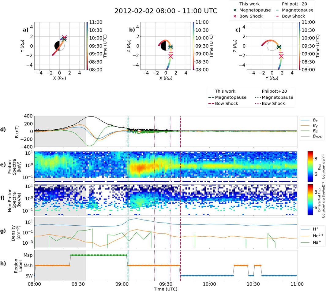
Figure 2. A 3-h window of MESSENGER data on 2012 February 02 from 08:00 to 11:00 UTC. Panels (A), (B), and (C) show the orbit of the spacecraft for this time period in the X-Y, X-Z, and Y-Z MSO planes, respectively, where the color bar represents the time and the green and magneta markers represent magnetopause and bow shock crossings respectively. For reference, the Philpott et al. (2020) crossings are shown as lines and the clustering algorithm transitions are shown as X’s. Plotted below are the observed quantities from MESSENGER: (D) magnetic field in MSO coordinates, (E) FIPS proton spectra, (F) FIPS spectra (excluding protons), and (G) number density of various ion species (
We include the non-proton spectrogram and multi-species densities for context, but note that these quantities are not included in the clustering algorithm. The non-proton spectrogram and ion densities indicate where MESSENGER is firmly within the magnetosphere. For example, where the
For reference, we also show times from the Philpott et al. (2020) catalog of visually identified bow shock and magnetopause crossings (hereafter referred to as the P20 catalog, marked by the dashed vertical lines in Figures 2D–H). Our identified magnetopause is in good agreement with P20, where the specific crossing time is within their magnetopause inner and outer boundary window. However, the bow shock identified by clustering is outside of the P20 bow shock outer boundary by
Figures 3A,B show the spatial extent of the three classifications of plasma regions labeled by the clustering in MSO coordinates when applied to the 4 years of MESSENGER data on the dayside. To better understand how the region and transition identifications are distributed, Figures 3A,B show different ranges of spatial coordinates for each of the two-dimensional planes. Specifically, for the X-Y plane (left column of Figure 3), the polar orbit of MESSENGER allows for investigation of the dayside regions at different latitudes. In the X-Y plane, we see that for low
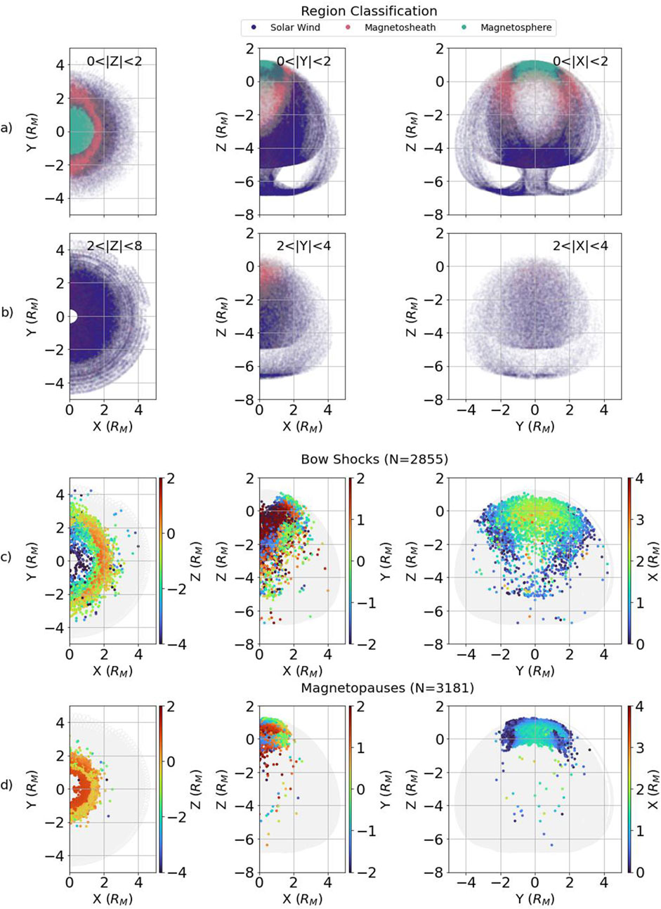
Figure 3. The spatial distribution of plasma regions and transitions identified through the clustering algorithm on Mercury’s dayside
Figures 3C,D show the locations of the bow shock and magnetopause crossings identified through clustering, where the color corresponds to the location in the out-of-plane dimension for that transition. The distribution of magnetopause crossings is inward of the bow shock crossings, as expected. Also, most of the magnetopause crossings identified in the MESSENGER data occur near the poles (seen most clearly in the X-Z plane of Figure 3D). This is likely due to the orbit of MESSENGER having periapses near the poles (
3.2 Comparison to published MESSENGER transition lists
Because this is an unsupervised learning model, there is no standard process to validate the model (e.g., Camporeale, 2019), as there are no ground truth labels from a training set. In lieu of this type of validation, we provide a comparison of the adapted T24 model against catalogs of manually validated MESSENGER bow shock and magnetopause crossing intervals. We compare our results to P20, which used 1-s resolution magnetometer data to visually identify 8,108 bow shock and 8,131 magnetopause crossings during the entirety of the MESSENGER mission. They employed the same identification approach as Winslow et al. (2013), hereafter W13, by identifying magnetopause and bow shock crossings marked by an increase in magnetic field magnitude, change in the magnetic field direction or rotation, or increased variability in the magnetic field components. For details on the identification of magnetopause and bow shock crossings in these studies, see W13. As noted in their study, the P20 list was visually identified and reviewed by multiple members of the MESSENGER team. We note also that despite being manually reviewed labels, these boundary identifications are not necessarily equivalent to ground truth labels and also suffer biases, as discussed in W13. However, it is of use to evaluate how these manually reviewed lists compare to the automated clustering list.
P20 marked a start and a stop time for each bow shock and magnetopause identified in their list. There are 3,888 bow shock crossings and 3,990 magnetopause crossings from P20 where the start and the stop times occur on the dayside
Since we identify a single, specific time for each magnetopause and bow shock crossing in this work, we compare to the P20 transitions using a match window for each boundary. For each P20 transition, the match window is the time period 3 min before the transition start to 3 min after the transition stop. A bow shock or magnetopause from our clustering algorithm is a match with a P20 bow shock or magnetopause if the time of the crossing occurs within this match window. We choose a 3-min buffer around the start and stop times to reflect the median time period between the start and stop of a transition boundary in the P20 list and to take into account the difference in temporal resolution between transitions identified in the clustering algorithm versus those identified through visual inspection in P20. We also only consider P20 transitions for comparison when less than 20% of the clustering region labels within the match window were labeled as “Unknown”, when there is adequate data for the clustering algorithm to determine the region on each side of the bow shock or magnetopause. We determine 3,552 bow shock crossings and 3,660 magnetopause crossings from the P20 list for comparison.
Using the match window criteria, we find that 1,923 out of 2,855 bow shock crossings (67%) matched a bow shock in the P20 list. Of those, 1,920 out of the 1,923 matched bow shock crossings were unique matches (i.e., when only one bow shock identification from this method was within 3 min of either the start or stop time from a P20 bow shock). In turn, we find that 1,647 P20 bow shock crossings do not have a match in our bow shock list (i.e., a transition identification missed by the clustering algorithm). If we assume the P20 list is a complete list of all bow shock crossings on the dayside of Mercury as observed by MESSENGER, we calculate that our bow shock identification is 54% complete. For magnetopause crossings, 2,355 out of 3,181 magnetopause crossings (74%) were matched to a P20 magnetopause crossing. All of the matched crossings were unique. We calculate a magnetopause identification completeness of 64%.
Our completeness criteria will depend on the time window we choose as a match window. If we choose a match window of 5 min instead of 3 min, we find that the bow shock match rate increases to 71% and the completeness rate is 57%, while the magnetopause match and completeness rate is 82% and 71%, respectively. The overall median time difference between our transition and the closest transition start or stop in the P20 list was 67 s for bow shock crossings and 64 s for magnetopause crossings, indicating that the majority of bow shock crossings and magnetopause crossings identified through the clustering approach is in good agreement with the P20 identifications. However, of the non-matching transitions, where the nearest P20 transition was separated by more than 3 min, we find that the median time difference is 19 min when comparing bow shock crossings and 6 min comparing magnetopause crossings, which suggests that our clustering approach is not as robust in identifying bow shock crossings as they would be if identified through visual inspection.
For comparison, without the relabeling rules applied in Table 1, there is a significant drop to 7%–22% match rates/completion rates which further underscores the necessity of these rules as a part of the model (comparison tables are provided in Supplementary Material). We emphasize that these relabeling rules are an improvement from simple rule based/threshold classifications, as they only modify the results when there is a specific initial clustering label and a condition that contradicts the validity of that label. A purely threshold based approach cannot easily handle, for instance, rare solar wind driving conditions. We note that the comparison to P20 does not serve as a traditional machine learning validation of the adapted T24 model, as P20 only marks the start and end times of transition regions rather than individually classifying each 1 min plasma region of MESSENGER’s dayside data.
We display the locations of our clustering matches with P20 in Figure 4, shown as a function of completeness. For a given spatial grid, we calculate the completeness as the number of P20 transitions that were also identified by clustering (e.g., completeness of 1 means all P20 transitions matched to a transition identified in clustering using the matching algorithm described above). For bow shock crossings, we find that the match completeness is relatively uniform in all spatial planes, though there is some spatial variation in the
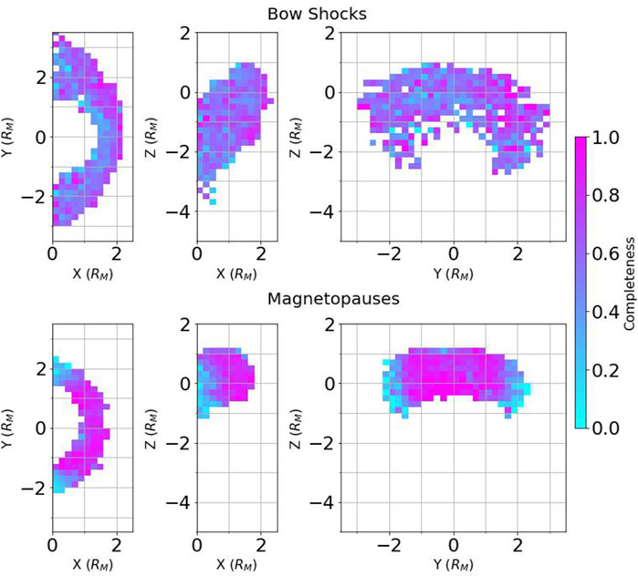
Figure 4. The fraction of intervals from Philpott et al. (2020) that were matched to a bow shock (top) or magnetopause (bottom) crossing identified from the clustering algorithm, shown in three spatial planes in MSO coordinates. Only cells with more than 5 transitions are plotted.
3.3 Bow shock and magnetopause model locations
We also compare the locations of the bow shock and magnetopause crossings identified in this work with the empirical bow shock and magnetopause models derived in W13 and P20, respectively. To directly compare our results to W13 and P20, we first correct for the aberration due to the solar wind flow and the offset from the planetary dipole. The aberration incorporates Mercury’s orbital velocity, which can vary based on the planet’s location in its eccentric orbit. To correct for aberration effects in the
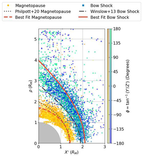
Figure 5. Bow shock crossings (blue to green squares) and magnetopause crossings (yellow to orange circles) identified from the clustering algorithm in the aberrated
Also shown in Figure 5 are the W13 bow shock and P20 magnetopause models as dashed-dot and dotted lines, respectively. The functional form of the W13 bow shock is adapted from Slavin et al. (2009) and is defined as
where
where
Figure 5 also includes fits to the bow shock (solid line) and magnetopause (dashed line) locations derived from our identified transitions using a least-squares method to compare to the W13 and P20 model fits. The bow shock crossings identified by the clustering algorithm lead to a best fit shape that is farther from Mercury and slightly more extended in
4 Summary and conclusion
We have automatically categorized all 4 years of dayside MESSENGER orbit data into three plasma regimes (magnetosphere, magnetosheath, and solar wind) at 1-min resolution. This was done using an unsupervised plasma region clustering model originally trained on dayside Earth observations from the MMS mission and fine tuned with MESSENGER data as a proof of concept that this Earth based model can be extended to different planetary environments and missions. In order to account for differences in both MESSENGER and MMS instrumentation and between Mercury and Earth’s magnetospheres, we applied additional post-cleaning rules and minimal changes to the generated features (e.g., changing the normalized value of
We compare our results against the Philpott et al. (2020) (P20) list of bow shock and magnetopause crossings that were visually identified using magnetic field data from the entire MESSENGER mission. Using an identification criteria that the plasma region remains stable for 3 min before and after each bow shock or magnetopause, we find that 67% of bow shock and 74% of magnetopause crossings that we identify also appear in the P20 list, with a total completeness of 54% and 64% for bow shock and magnetopause identifications, respectively. For magnetopause crossings, the completeness is dependent on location, where we find a lower match to the P20 magnetopause list near the flanks. Similarly, we find good agreement in the 2D shape of the magnetopause except at the flanks, where we find less flaring of the fitted magnetopause location than reported in P20. For bow shock crossings, the most representative 2D shape from the bow shock crossings identified in this work extends further out from the surface of Mercury than that previously described in Winslow et al. (2013) (W13), and we find a larger spread in the spatial distribution of our identified bow shock crossings. We note that we are not trying to recreate or exceed manual methods for identifying plasma regions from MESSENGER, but instead we are focused on demonstrating that an extensible unsupervised learning model trained on Earth-based data can be successfully applied to vastly differing conditions and missions. This method also can provide an initial identification of interesting events or regions for further study which may be useful for the upcoming BepiColombo mission.
Future work will include in-depth parameter sensitivity studies of the T24 model features and comparisons with use of T24 with no modifications to further identify the main observational drivers that benefit or limit the completeness and accuracy of the clustering algorithm. This includes extending the T24 model dataset as long as available with MMS for years within the ascending and maximum phases of the solar cycle to account for any possible biases related to primarily sampling solar minimum conditions and also upsampling rare solar wind conditions. Additionally, future work will seek to better optimize the algorithm for nightside observations to enable further studies of magnetospheric regions and dynamics. Finally, future efforts will also focus on adapting the clustering algorithm to observations at different planets, including the largely rotationally-driven intrinsic magnetospheres of the outer planets and the induced magnetosphere of Venus.
Data availability statement
The datasets presented in this study can be found in online repositories. The names of the repository/repositories and accession number(s) can be found below: https://zenodo.org/records/13904008 (Toy-Edens et al. 2024a).
Author contributions
VT-E: Writing – original draft, Writing – review and editing, Conceptualization, Data curation, Formal Analysis, Investigation, Methodology, Software, Validation, Visualization. WM: Writing – review and editing, Conceptualization, Data curation, Formal Analysis, Investigation, Methodology, Software, Validation, Visualization. RA: Writing – review and editing, Conceptualization, Funding acquisition, Project administration, Supervision. SV: Writing – review and editing, Conceptualization, Supervision. SR: Writing – review and editing.
Funding
The author(s) declare that financial support was received for the research and/or publication of this article. This study was supported by NASA grants 80NSSC19K0789 and 80NSSC22K0993. SR acknowledges the support by Johns Hopkins University Applied Physics Laboratory independent R&D.
Acknowledgments
The authors would like to thank George Ho and Drew Turner for their support.
Conflict of interest
The authors declare that the research was conducted in the absence of any commercial or financial relationships that could be construed as a potential conflict of interest.
The author(s) declared that they were an editorial board member of Frontiers, at the time of submission. This had no impact on the peer review process and the final decision.
Generative AI statement
The author(s) declare that no Generative AI was used in the creation of this manuscript.
Publisher’s note
All claims expressed in this article are solely those of the authors and do not necessarily represent those of their affiliated organizations, or those of the publisher, the editors and the reviewers. Any product that may be evaluated in this article, or claim that may be made by its manufacturer, is not guaranteed or endorsed by the publisher.
Supplementary material
The Supplementary Material for this article can be found online at: https://www.frontiersin.org/articles/10.3389/fspas.2025.1608091/full#supplementary-material
References
Anderson, B. J., Acuña, M. H., Lohr, D. A., Scheifele, J., Raval, A., Korth, H., et al. (2007). The magnetometer instrument on messenger. Space Sci. Rev. 131, 417–450. doi:10.1007/s11214-007-9246-7
Andrews, G. B., Zurbuchen, T. H., Mauk, B. H., Malcom, H., Fisk, L. A., Gloeckler, G., et al. (2007). The energetic particle and plasma spectrometer instrument on the MESSENGER spacecraft. Space Sci. Rev. 131, 523–556. doi:10.1007/s11214-007-9272-5
Benkhoff, J., Murakami, G., Baumjohann, W., Besse, S., Bunce, E., Casale, M., et al. (2021). Bepicolombo - mission overview and science goals. Space Sci. Rev. 217, 90. doi:10.1007/s11214-021-00861-4
Brown, C. P., Maruca, B. A., Prabakaran, V., Qudsi, R. A., Walsh, B. M., Alterman, B. L., et al. (2025). Evaluating the parker model with the trans-heliospheric survey. Geophys. Res. Lett. 52, e2025GL115186. doi:10.1029/2025gl115186
Burch, J. L., Moore, T. E., Torbert, R. B., and Giles, B. L. (2015). Magnetospheric multiscale overview and science objectives. Space Sci. Rev. 199, 5–21. doi:10.1007/s11214-015-0164-9
Camporeale, E. (2019). The challenge of machine learning in space weather: nowcasting and forecasting. Space weather. 17, 1166–1207. doi:10.1029/2018sw002061
Chané, E., Raeder, J., Saur, J., Neubauer, F. M., Maynard, K. M., and Poedts, S. (2015). Simulations of the earth's magnetosphere embedded in sub-Alfvénic solar wind on 24 and 25 may 2002. J. Geophys. Res. Space Phys. 120, 8517–8528. doi:10.1002/2015ja021515
Chen, Y., Dong, C., and Sun, W. (2024). Transport and distribution of sodium ions in mercury’s magnetosphere: results from multi-fluid mhd simulations. Geophys. Res. Lett. 51. doi:10.1029/2024gl110301
Dungey, J. W. (1961). Interplanetary magnetic field and the auroral zones. Phys. Rev. Lett. 6, 47–48. doi:10.1103/PhysRevLett.6.47
Gershman, D. J., Zurbuchen, T. H., Fisk, L. A., Gilbert, J. A., Raines, J. M., Anderson, B. J., et al. (2012). Solar wind alpha particles and heavy ions in the inner heliosphere observed with messenger. J. Geophys. Res. Space Phys. 117. doi:10.1029/2012ja017829
Hajra, R., and Tsurutani, B. T. (2022). Near-earth sub-alfvénic solar winds: interplanetary origins and geomagnetic impacts. Astrophysical J. 926, 135. doi:10.3847/1538-4357/ac4471
Ip, W. H. (1990). On solar radiation–driven surface transport of sodium atoms at mercury. Astrophysical J. 356, 675. doi:10.1086/168874
James, M. K., Imber, S. M., Raines, J. M., Yeoman, T. K., and Bunce, E. J. (2020). A machine learning approach to classifying messenger fips proton spectra. J. Geophys. Res. Space Phys. 125, e2019JA027352. doi:10.1029/2019JA027352
Johnson, C. L., Anderson, B. J., Korth, H., Phillips, R. J., and Philpott, L. C. (2018). “Mercury’s internal magnetic field,” in Mercury. The view after MESSENGER. Editors S. C. Solomon, L. R. Nittler, and B. J. Anderson, 114–143. doi:10.1017/9781316650684.006
Lavraud, B., and Borovsky, J. E. (2008). Altered solar wind-magnetosphere interaction at low mach numbers: coronal mass ejections. J. Geophys. Res. Space Phys. 113. doi:10.1029/2008ja013192
Leblanc, F., and Johnson, R. (2003). Mercury’s sodium exosphere. Icarus 164, 261–281. doi:10.1016/S0019-1035(03)00147-7
Philpott, L. C., Johnson, C. L., Anderson, B. J., and Winslow, R. M. (2020). The shape of mercury’s magnetopause: the picture from messenger magnetometer observations and future prospects for bepicolombo. J. Geophys. Res. Space Phys. 125, e2019JA027544. doi:10.1029/2019JA027544
Raines, J. M., Gershman, D. J., Zurbuchen, T. H., Sarantos, M., Slavin, J. A., Gilbert, J. A., et al. (2013). Distribution and compositional variations of plasma ions in mercury’s space environment: the first three Mercury years of messenger observations. J. Geophys. Res. Space Phys. 118, 1604–1619. doi:10.1029/2012ja018073
Shue, J. H., Song, P., Russell, C. T., Steinberg, J. T., Chao, J. K., Zastenker, G., et al. (1998). Magnetopause location under extreme solar wind conditions. J. Geophys. Res. Space Phys. 103, 17691–17700. doi:10.1029/98JA01103
Slavin, J. A., Acuña, M. H., Anderson, B. J., Barabash, S., Benna, M., Boardsen, S. A., et al. (2009). Messenger and Venus express observations of the solar wind interaction with Venus. Geophys. Res. Lett. 36. doi:10.1029/2009GL037876
Slavin, J. A., Imber, S. M., and Raines, J. M. (2021). “A dungey cycle in the life of mercury’s magnetosphere,”, 34. American Geophysical Union AGU, 535–556. doi:10.1002/9781119815624.ch34
Solomon, S. C., McNutt, R. L., Gold, R. E., and Domingue, D. L. (2007). MESSENGER mission overview. Space Sci. Rev. 131, 3–39. doi:10.1007/s11214-007-9247-6
Sun, W., Dewey, R. M., Aizawa, S., Huang, J., Slavin, J. A., Fu, S., et al. (2022). Review of Mercury’s dynamic magnetosphere: post-MESSENGER era and comparative magnetospheres. Sci. China Earth Sci. 65, 25–74. doi:10.1007/s11430-021-9828-0
Toy-Edens, V., Mo, W., Allen, R., Vines, S., and Raptis, S. (2024a). enAutomated messenger plasma region classifications via unsupervised transfer learning. doi:10.5281/zenodo.13904008
Toy-Edens, V., Mo, W., Raptis, S., and Turner, D. L. (2024b). Classifying 8 years of mms dayside plasma regions via unsupervised machine learning. J. Geophys. Res. Space Phys. 129, e2024JA032431. doi:10.1029/2024ja032431
Winslow, R. M., Anderson, B. J., Johnson, C. L., Slavin, J. A., Korth, H., Purucker, M. E., et al. (2013). Mercury’s magnetopause and bow shock from MESSENGER magnetometer observations. J. Geophys. Res. (Space Phys.) 118, 2213–2227. doi:10.1002/jgra.50237
Keywords: messenger, machine learning, unsupervised learning, transfer learning, plasma, MMS, bow shock, magnetopause
Citation: Toy-Edens V, Mo W, Allen RC, Vines SK and Raptis S (2025) Automated classification of MESSENGER plasma observations via unsupervised transfer learning. Front. Astron. Space Sci. 12:1608091. doi: 10.3389/fspas.2025.1608091
Received: 08 April 2025; Accepted: 10 July 2025;
Published: 22 July 2025.
Edited by:
Chuanfei Dong, Boston University, United StatesReviewed by:
Verena Heidrich-Meisner, University of Kiel, GermanyDonglai Ma, University of California, Los Angeles, United States
Copyright © 2025 Toy-Edens, Mo, Allen, Vines and Raptis. This is an open-access article distributed under the terms of the Creative Commons Attribution License (CC BY). The use, distribution or reproduction in other forums is permitted, provided the original author(s) and the copyright owner(s) are credited and that the original publication in this journal is cited, in accordance with accepted academic practice. No use, distribution or reproduction is permitted which does not comply with these terms.
*Correspondence: Vicki Toy-Edens , Vmlja2kuVG95LUVkZW5zQGpodWFwbC5lZHU=