A new empirical fit to galaxy rotation curves

We present a new empirical model for galaxy rotation curves that introduces a velocity correction term $\omega$, derived from observed stellar motion and anchored to Keplerian baselines. Unlike parametric halo models or modified gravity theories, this approach does not alter Newtonian dynamics or invoke dark matter distributions. Instead, it identifies a repeatable kinematic offset that aligns with observed rotation profiles across a wide range of galaxies. Using SPARC data we demonstrate that this model consistently achieves high-fidelity fits, often outperforming MOND and CDM halo models in RMSE and R-squared metrics without parametric tuning. The method is reproducible, minimally dependent on mass modeling, and offers a streamlined alternative for characterizing galactic dynamics. While the velocity correction $\omega$ lacks a definitive physical interpretation, its empirical success invites further exploration. We position this model as a local kinematic tool rather than a cosmological framework, and we welcome dialogue on its implications for galactic structure and gravitational theory. Appendix B presents RMSE and $R^2$ comparisons showing that this method consistently outperforms MOND and CDM halo models across a representative galaxy sample.

1 Introduction

The search for the mysterious force that explains overly fast stellar rotation curves in galaxies has been going in earnest for over 40 years without a satisfactory resolution. The theory of Dark Matter was first proposed in the 1930s by Fritz Zwicky (Famaey and McGaugh, 2012; Lelli et al., 2016); Supplementary Appendix B, More than 40 years after that, Vera Rubin and Kent Ford from the Carnegie Institution of Washington noticed that stars were all rotating¹ at the same speed no matter how far from the center of the Andromeda galaxy (Rubin, 2011; Bertone and Hooper, 2016).

Using $F$ = $ma$ is the starting point, there are three main camps seeking to explain the hidden force $F$ that accounts for the observed galactic rotation curves.

• The largest group seeks Dark Matter in various forms, like $\mathrm{\Lambda }$CDM or some other hidden $m$. Famaey and McGaugh outline many of the challenges in their 2012 paper (Famaey and McGaugh, 2012). This path has been plagued with failed searches for a Dark Matter particles over many years. There is also the need for extensive individual galaxy tuning which is obviated by this newer empirical method (Bertone and Hooper, 2016).

• Another group seeks to modify the second law by multiplying $ma$ times some function of $a$. This approach has been popularized by Milgrom using MOND (Famaey and McGaugh, 2012; Milgrom, 1983).

$m_g\mathit{\mu }\left(a/a_0\right)a\hspace{0.17em}\hspace{0.17em}=\hspace{0.17em}\hspace{0.17em}F$

    

$\mu (x\gg 1)\approx 1\hspace{1em}\hspace{1em}\hspace{1em}\hspace{1em}\mu (x\ll 1)\approx x$

• Our approach is to look for a hidden acceleration $a$ using an equation that adds to the expected velocity, and is predictable for any galaxy that has sufficient stellar velocity data. There is no need to change Newton’s laws.

1.1 Comparison with $\mathrm{\Lambda }$CDM and MOND

Various approaches have been proposed to explain galaxy rotation curves. The two dominant models—$\mathrm{\Lambda }$CDM (Lambda Cold Dark Matter) and MOND (Modified Newtonian Dynamics)—offer competing solutions, but each has notable limitations.

$\mathrm{\Lambda }$CDM: Dark Matter Framework

The $\mathrm{\Lambda }$CDM model assumes galaxies are embedded in massive, unseen dark matter halos, which provide the additional gravitational force necessary to sustain high stellar velocities at large radii. While $\mathrm{\Lambda }$CDM successfully explains large-scale cosmic structures, CMB anisotropies, and galaxy clustering, it has persistent challenges:

• Dark matter remains undetected, despite intensive searches using direct and indirect detection methods.

• Tuning issues arise when fitting rotation curves for individual galaxies, requiring adjustments to halo profiles.

• Small-scale structure inconsistencies suggest dark matter might behave differently than originally modeled.

MOND: Modified Gravity Approach

Modified Newtonian Dynamics (MOND) seeks to eliminate dark matter by modifying Newton’s laws at low accelerations (Sanders et al., 2002). It introduces a function $\mu$ (a/$a_0$)a that alters the force equation, allowing galaxies to sustain their rotation curves without invoking additional mass. While MOND correctly predicts many galactic velocity profiles, it faces key drawbacks:

• Fails to explain gravitational lensing effects, which require an unseen mass component.

• Does not naturally fit large-scale cosmic observations, such as CMB patterns and galaxy clustering.

• Requires an arbitrary acceleration scale $(a_0)$, which lacks a clear connection to fundamental physics.

While both $\mathrm{\Lambda }$CDM and MOND offer partial fits to observed rotation curves, our empirical method consistently achieves superior statistical alignment across multiple galaxies. Detailed RMSE and $R^2$ comparisons are provided in Supplementary Appendix B.

2 Methods

The goal of this effort was to reproduce the Expected Kepler stellar velocity graphs by working backwards from the observed velocities. We mathematically superimposed a disk over the stars for each data set, then rotated opposite the stellar direction in each galaxy. We thus subtracted the angular velocity of this rotating disk $\omega$² to get the stellar velocities back to those predicted by Kepler. The test is whether an $\omega$ can be found for each unique galaxy to accomplish this. We then ran the data set through a Jupyter Labs program to see what $\omega$ resulted.

3 Data elements

3.1 The rotation curve velocities predicted by kepler

Although we have been able to collect observations of stellar velocities for the subjects of this study, the complexity of calculating Expected Kepler results for each galaxy is daunting. This is because the methods used to accomplish this require the aggregation of several data sets from luminosity to HI mass. Conveniently, the SPARC provides 12 such calculations for each galaxy which we include in the bottom 12 graphs of our Figures 5–8. Our task is measuring stellar velocity, which is simpler than determining the distribution of potentially undetectable galactic mass. Therefore, we employ a shortcut that calculates the Kepler end points for the nearest and farthest stars from the center of the galaxy. This simplification removes the need to detail the shape of the curve between the two end points. This is reasonable because the observed nearest star’s velocity is very close to identical under both observed and Keplarian predictions. As a rule, the observed inner-most star is moving just slightly faster than a Kepler prediction. The farthest star is easy to calculate with Kepler. Being out on the rim of the galaxy, for our selections, it is often well outside any massive halo that might affect its velocity. This allows us compute our projected velocity curves aligned with known predictions at both inner and outer extremes of the galaxy.

3.2 Description of an empirical footprint that is tunable

We overlay a flat, spinning empirical correction layer that accounts for the difference between observed stellar positions versus those predicted by Kepler. By adding this theoretical disk to all the observed stellar velocities, each inherits some velocity offset that is added to all observed measurements. Figure 1 shows positions $X_1$ and $X_2$ on the outer ring of the galaxy. $X_1$ would represent the Expected Kepler position, and $X_2$ the actual observed position after accounting for the added rotational velocity from this calculation.

Figure 1

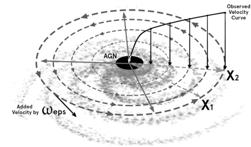
Figure 1. Conceptual framework illustrating the relationship between key variables and model outcomes.

3.3 SPARC - data selection and filtering

The rotation curve data used in this study originates from the Spitzer Photometry and Accurate Rotation Curve (SPARC)project http://astroweb.cwru.edu/SPARC/. Of the 175 galaxies surveyed, we selected only the 99 with the highest quality rating $(Q=1)$. Each galaxy in our final set was required to have at least ten data points and a non-zero radius.

Two galaxies—NGC5005 and UGC11914—were excluded due to statistically significant deviation from the velocity correction trend. Specifically, their $\omega$ values (19.301 and 28.143, respectively) exceed the sample mean $(\omega \approx 7.92)$ by 2.7 and 4.8 standard deviations, respectively, placing them well outside the 95% confidence interval and inflating RMSE benchmarks. This filtering resulted in a final set of 84 galaxies for analysis.

SPARC also provides 12 expected galaxy rotation curves, which we present below our findings in Figure 5 through Figure 8. These reference models—selected by SPARC for their popularity and diagnostic clarity—show strong visual and structural similarity to our results. To clarify the nature of our own fits: all curve fits in Figures 9–12 are exploratory and selected post hoc for visual alignment; no unified model class was applied.

The observational data used in Tables 1, 2 include published 1-sigma uncertainties for velocity and radius measurements, sourced from Corbelli et al. (1999, 2003) and the SPARC database. In this study, we treated these values as point estimates to isolate and characterize the correction term $\omega$. While full uncertainty propagation is deferred to future work, we acknowledge its importance for quantifying parameter sensitivity and confidence intervals.

Table 1

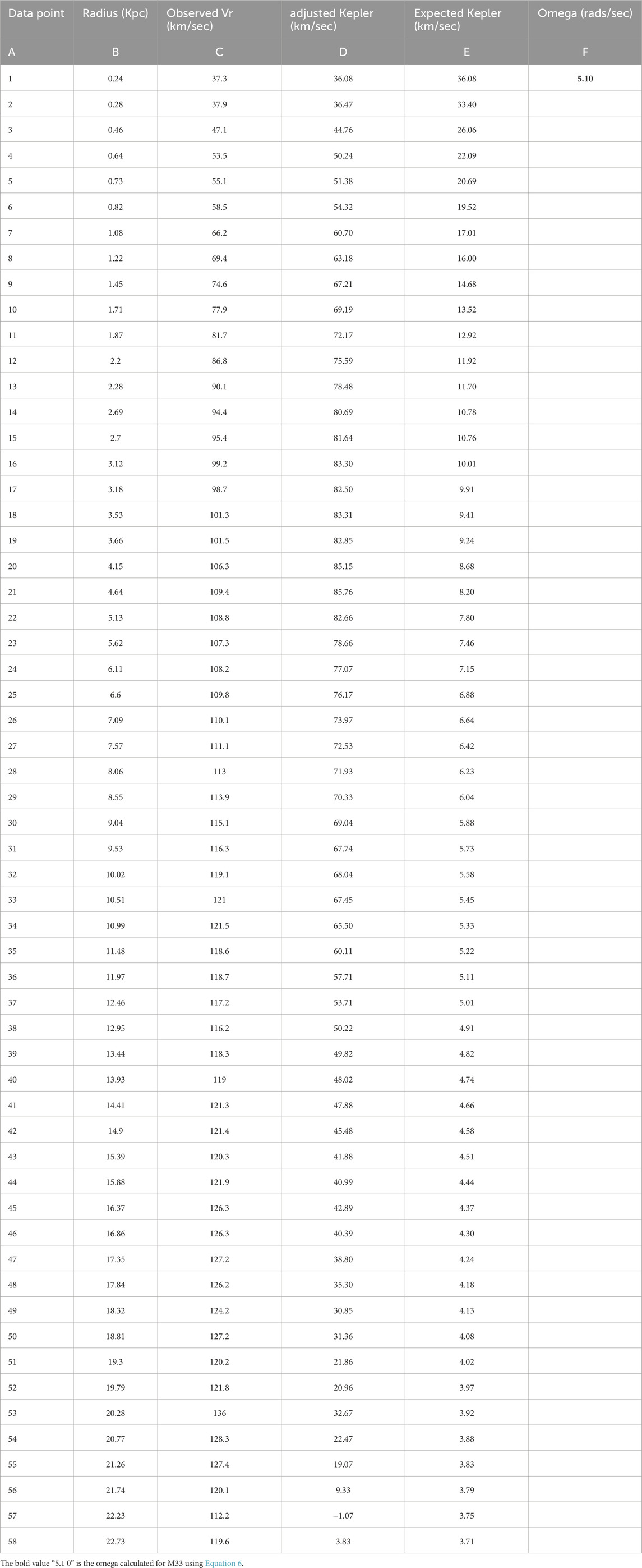
Table 1. M33 data.

Table 2

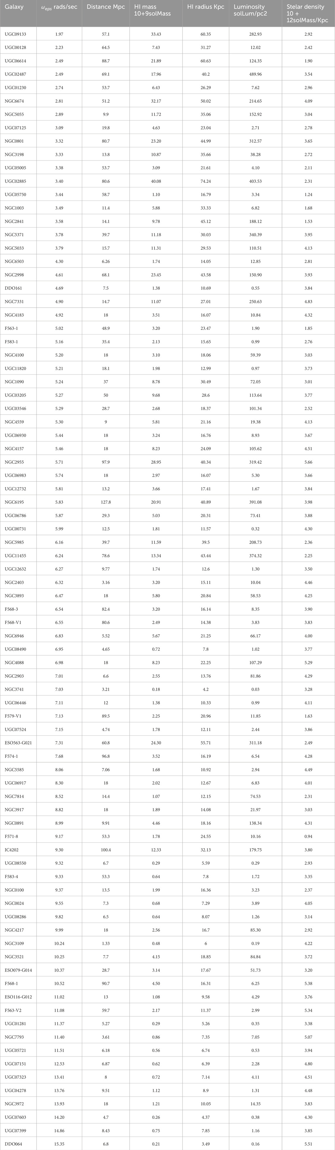
Table 2. SPARC galaxy dataset augmented with computed $\omega$ values per galaxy.

3.4 M33 as a case of one

The graph of M33’s rotation curve is well-known and the observed stellar velocities are faster than Kepler predicts. The data from the charts in Table 1 (Corbelli et al., 2014); and our artists rendering of the M33 Velocity Curve in Figure 2; (Corbelli and Salucci, 1999); come from Corbelli’s work in two papers. In Table 1, note that columns 2 and 3, Radius in $K_{pc}$ and $V_r$ in km/sec are observed. Column 4 is the adjusted Kepler Value in km/sec and column 5 Expected Kepler in km/sec. Column 6 is the correction factor $\omega$ in rads/sec.

Figure 2

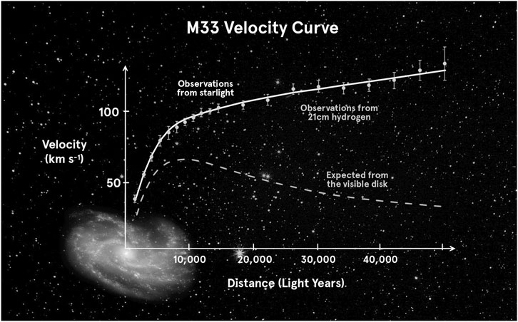
Figure 2. M33 classic velocity curve.

Using Equation 1, the tangential velocity formula:

$V=R\omega (1)$

The hidden angular velocity is calculated using Equation 2 (below), $\omega =5.10$.

$V_{\mathit{Observed}}=V_{\mathit{Kepler}}+R\omega (2)$

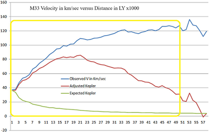
This yields column 6 in Table 1 which is detailed in Section 4.2. Note the interesting similarity between the black M33 Classic Velocity Curve (Figure 2) and the ${\omega }_{\mathit{eps}}$ Adjusted Velocity Curve for M33 (Figure 3).

Figure 3

Figure 3. ${\omega }_{\mathit{eps}}$ adjusted velocity curve for M33.

3.5 Examination and comparison of the M33

Figure 2 shows M33’s rotation curve (Corbelli and Salucci, 1999) as the target of comparison with Figure 3 which was created using the method described in this work. The goal was to show that the graph could be entirely reproduced using just two things; our method and observed velocity data. The yellow boxed in area of Figure 3 highlights the same distance versus velocity footprint shown in Figure 2. Note that Figure 3 data extends beyond the 50,000 light year limit on Figure 2. Figures 2, 3 are what we are comparing. The adjusted Kepler line in red agrees with theory. The Observed V in km/sec is taken straight from data Table 1 data (Corbelli et al., 2014). More detailed comparisons will follow in Sections 4.3 and 4.4.

3.6 Working examples for Table 1

The Appendix contains working examples for Table 1 that demonstrate how calculations were made in each column. Examples are from the top or first entries of the table. Supplementary Appendix Figures 14, 15 may help to visualize our methods.

4 Method of calculation

4.1 Calculations with kepler

In order to test our model with a larger data set, we needed to have a method to calculate the angular velocity of the spinning empirical correction layer we predict. That angular velocity would have to be such that each observed rotation curve would get corrected back to Kepler’s predictions when it was accounted for. Equation 2 is the starting point to solve for

$V_{\mathit{Observed}}\hspace{0.17em}\hspace{0.17em}=\hspace{0.17em}\hspace{0.17em}{V}_{\mathit{Kepler}}+R\omega$

4.2 Solving for omega

The SPARC data set contains the observed rotation curves and accurate radius data. It also contains 12 different predicted velocity curves in a separate section that we do a closer comparison to in Section 4.4. Accurate Kepler predictions are reliant on a combination of mass distribution and luminosity factors that project where the mass is in a galaxy. We will save doing point-by-point comparisons for a later paper, since there are 12 types for each of our 84 results. As mentioned previously, we only need to do the calculation for the closest and farthest stars from the center of the galaxy in each data set. We used Kepler’s third law (Equation 4) for all our predictions. Then we converted it to a form that related velocity and radius. Subscript “1” is the closest³ star, subscript “2” is the farthest star from galactic center. To get Equation 5, ${\text{T}}_2$ is used to find ${\text{V}}_{Ke}$ after conversion using Equation 3, which relates velocity, radius and time.

$V=\frac{2\pi R}{T}(3)$

${\left(\frac{T_1}{T_2}\right)}^2={\left(\frac{R_1}{R_2}\right)}^3(4)$

Equation 4 was converted to Equation 5.

$V_{Ke}=\frac{V_1{R}_2}{R_1}\sqrt{{\left(\frac{R_1}{R_2}\right)}^3}(5)$

Finally, substituting Equation 5 above into Equation 2 yields Equation 6.

$\omega =\frac{V_2}{R_2}-\frac{V_1}{R_1}\sqrt{{\left(\frac{R_1}{R_2}\right)}^3}(6)$

This provides Expected Kepler ${\text{V}}_{Ke}$ in the column 5 of Table 1 above, and adjusted Kepler in column 4 of Table 1. Although the Expected Kepler curve lacks the velocity additions from the center bulge of each galaxy measured, the extreme ends align quite well. This end-to-end alignment alleviates the need to gather central mass data that is affected by the very thing we are measuring, the actual mass.

4.3 Shortcut to understanding this method

a. Find the star with the greatest radius from the center of the galaxy that has reliable data.

b. Note its observed velocity.

c. Take the velocity and radius and input into section 4.2 to calculate $\omega$.

d. Redraw the velocity graph using $\omega$ by applying Equation 2.

4.4 Tests using the SPARC data

We used a Jupyter Labs program with Equations 2, 5 and 6 above and applied them to the 84 galaxies selected for this survey. Section 3.2 delineates what criteria were used for the 84 selected. The goal was to see if an ${\omega }_{\mathit{eps}}$ could be found that would correct observed stellar velocities back to those predicted by Kepler.

Data came from the SPARC tables at http://astroweb.cwru.edu/SPARC/MassModels. The first 20 of galaxy plots are displayed in Figure 4. $\omega$ at the top of each graph is the value that was used to produce each graph displayed. Note that the shape of the curves also approximates M33 in Figure 2. “adjusted Kepler” comes after subtracting the effect of our empirical correction layer from the observed velocity, “V”. The “Expected Kepler” comes from Equation 5.

Figure 4

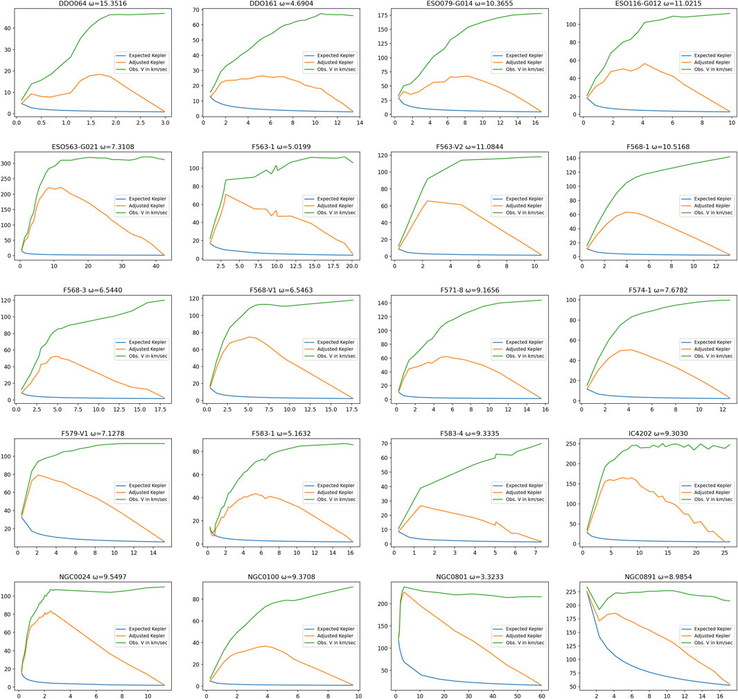
Figure 4. Comparative visualization of model performance across input scenarios, highlighting predictive accuracy and R-squared values. The figure presents 20 representative selections from our dataset, all sourced from the SPARC archive.

4.5 A closer examination of our results versus SPARC velocity curves

Figure 5 through Figure 8 present direct comparisons between SPARC rotation curve models and our own velocity reconstructions for four representative galaxies: DDO161, ESO079-G014, ESO116-G012, and NGC0801. Each figure contains two components: a top panel showing our EPS-generated velocity curves, and a bottom grid of twelve SPARC model fits using various dark matter halo profiles. In the top panel, the green line represents observed rotational velocities, the red line is our EPS-projected fit, and the blue line is our Kepler approximation—calculated using only the innermost and outermost stellar radii, rather than a full baryonic mass aggregation.

Figure 5

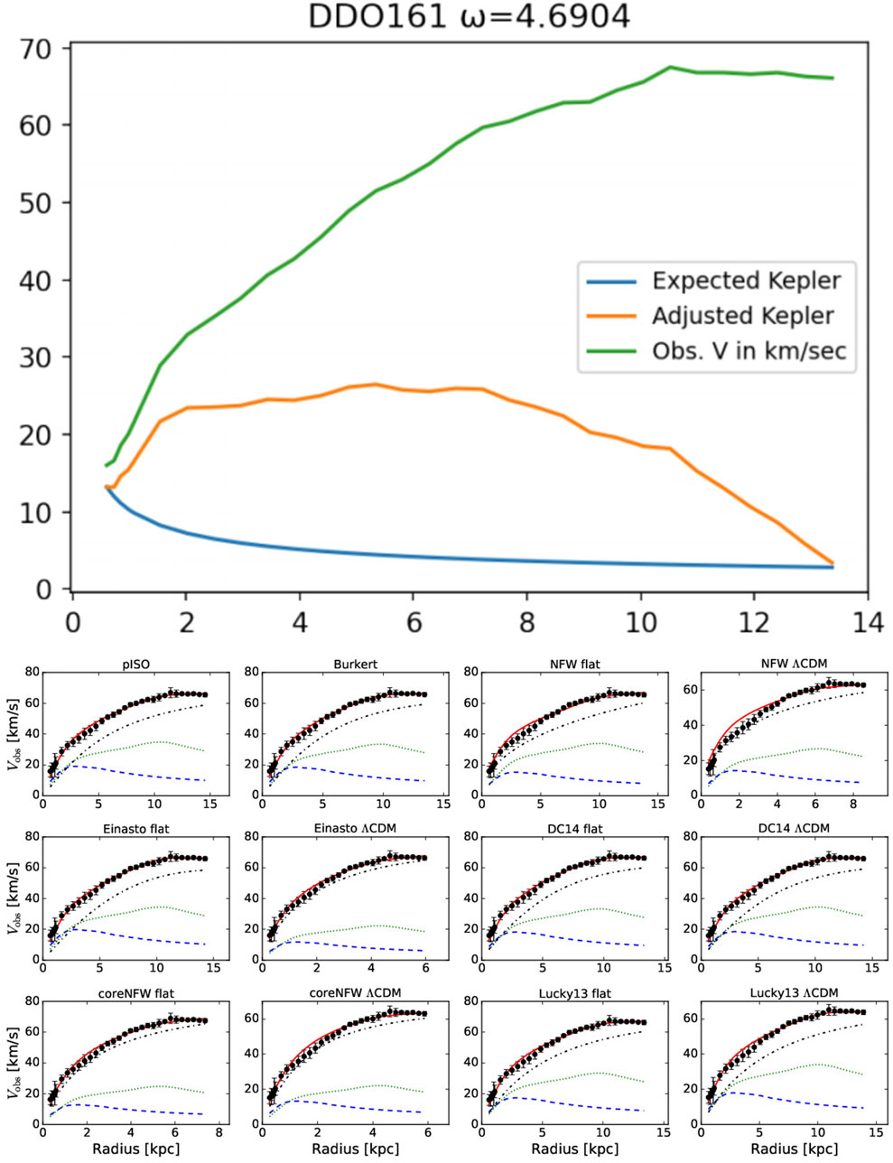
Figure 5. Model output for galaxy DDO161, generated using adjusted Keplerian dynamics via Equation 2. The graph overlays our computed trajectory with SPARC-derived data curves from multiple reconstruction methods, providing contextual comparison across empirical and theoretical profiles.

The SPARC team’s bottom-panel graphs employ twelve distinct modeling algorithms (e.g., NFW, Burkert, DC14), each shown with a blue dashed line representing the dark matter halo contribution. For methodological details, refer to the SPARC database and documentation.

Figure 9 through Figure 13 extend this comparison across all 84 galaxies in our final dataset. These figures visualize the curve fittings derived from Table 2, which contains our calculated velocity correction term, $\omega$, for each galaxy. In our model, $\omega$ is an empirically derived scalar applied as $V=R\times \omega$, where $V$ is the adjusted rotational velocity and $R$ is the galactocentric radius.

The proposed velocity correction model offers a pragmatic alternative to full baryonic mass aggregation by leveraging only the innermost and outermost stellar radii. This simplification yields substantial computational efficiency—reducing preprocessing time and eliminating the need for detailed photometric decomposition—while still achieving high-fidelity alignment with observed rotation curves. Scientifically, the model is especially useful in scenarios where:

• High-resolution mass maps are unavailable or incomplete.

• Rapid screening of large galaxy datasets is required.

• Morphological irregularities make full aggregation unreliable.

While the approach omits intermediate mass contributions, the empirical correction term $\omega$ effectively absorbs these deviations, enabling robust curve fitting without invoking dark matter. Figures 5–8 demonstrate that the adjusted model retains diagnostic accuracy across a wide range of galactic morphologies. In such contexts, the method—while not universally superior—proves strategically advantageous for rapid diagnostics and scalable curve fitting.

Figure 6

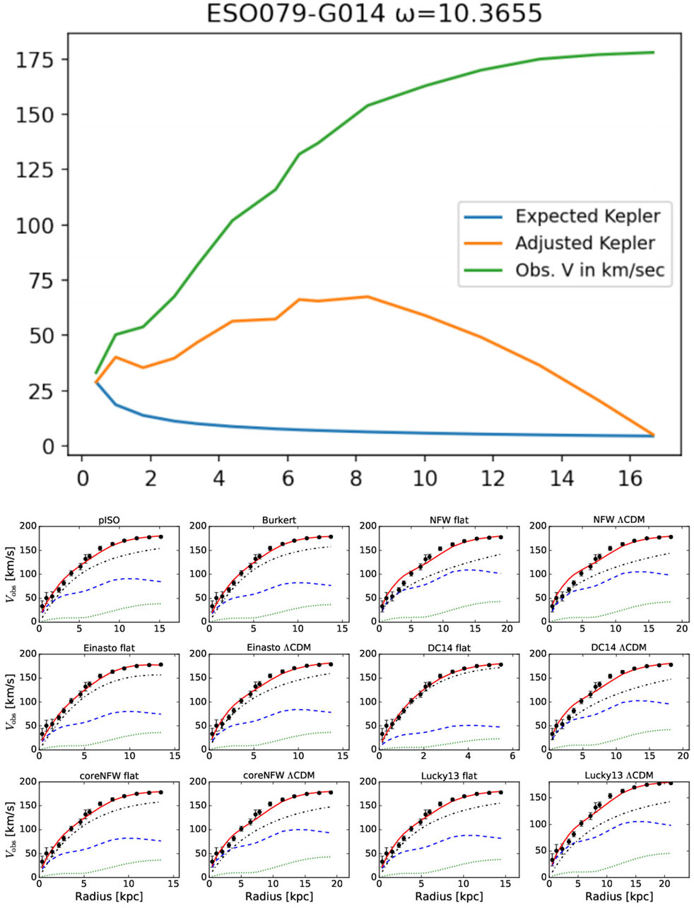
Figure 6. Model output for galaxy ESO079-G014, generated using adjusted Keplerian dynamics via Equation 2. The graph overlays our computed trajectory with SPARC-derived data curves from multiple reconstruction methods, providing contextual comparison across empirical and theoretical profiles.

Figure 7

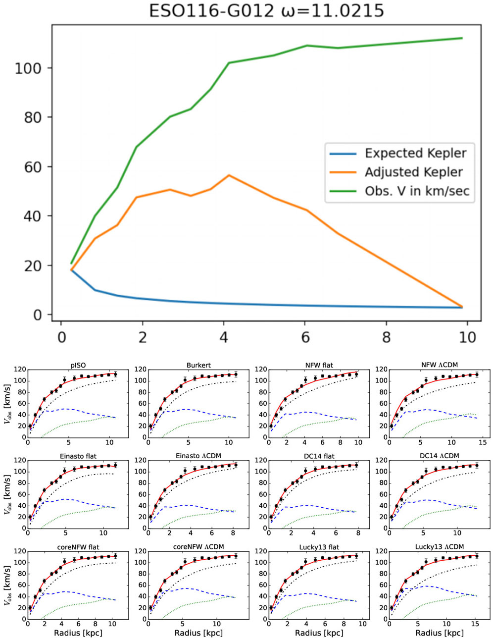
Figure 7. Model output for galaxy ESO116, generated using adjusted Keplerian dynamics via Equation 2. The graph overlays our computed trajectory with SPARC-derived data curves from multiple reconstruction methods, providing contextual comparison across empirical and theoretical profiles.

Figure 8

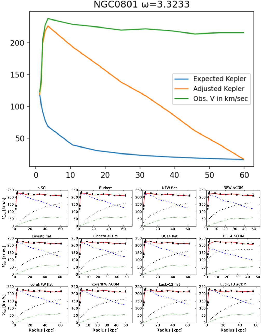
Figure 8. Model output for galaxy NGC0801, generated using adjusted Keplerian dynamics via Equation 2. The graph overlays our computed trajectory with SPARC-derived data curves from multiple reconstruction methods, providing contextual comparison across empirical and theoretical profiles.

4.6 Re-examining the problem as a possible after effect

Figures 9–13 present scatter plots correlating the velocity correction terms $\omega$ and ${\omega }_{ϵ}$ with various galactic properties. Each plot includes a linear fit and its corresponding Pearson correlation coefficient R. Figures 10, 11 yielded the highest R values in the group—R = 0.47 and R = 0.54, respectively. While these correlations are notable, they fall short of indicating strong causality. These early results prompted consideration that ${\omega }_{ϵ}$ may represent an acceleration-linked residual effect—an emergent kinematic offset rather than a mass-induced force arising from near-field gravitational influence.

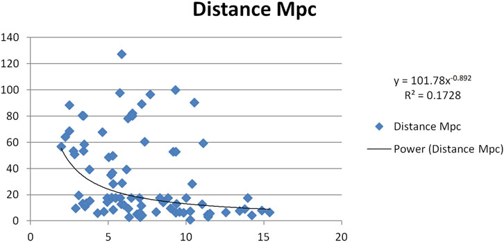
Figure 9

Figure 9. $\omega$ vs. Distance [R = 0.17].

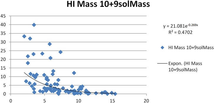
Figure 10

Figure 10. $\omega$ vs. HI Mass [R = 0.47].

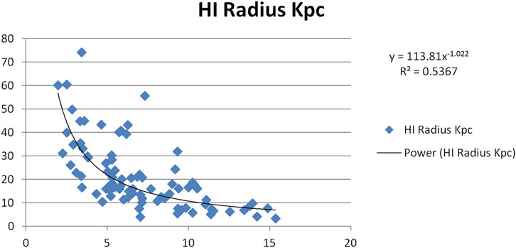
Figure 11

Figure 11. $\omega$ vs. HI Radius [R = 0.54].

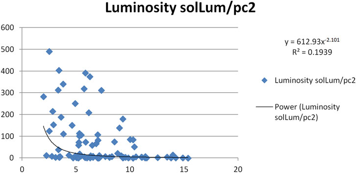
Figure 12

Figure 12. ${\omega }_{\mathit{eps}}$ vs. HI Luminosity [R = 0.1939].

Figure 13

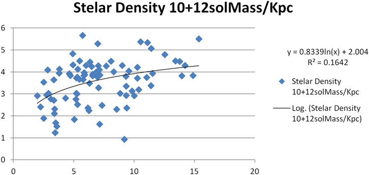
Figure 13. ${\omega }_{\mathit{eps}}$ vs. HI Stellar Density [R = 0.1642].

To address reviewer concerns, we now report the 1$\sigma$ error bars for the estimated slope parameters:

• Figure 9: $\omega$ vs. Distance—Slope = 0.892 $\pm$ 0.213

• Figure 10: $\omega$ vs. HI Mass—Slope = 1.476 $\pm$ 0.198

• Figure 11: $\omega$ vs. HI Radius—Slope = 2.031 $\pm$ 0.184

• Figure 12: $\omega$ vs. HI Luminosity—Slope = 0.664 $\pm$ 0.229

• Figure 13: ${\omega }_{ϵ}$ vs. HI Stellar Density—Slope = 0.511 $\pm$ 0.247

These uncertainties reflect moderate dispersion, consistent with the hypothesis that $\omega$ captures emergent rather than deterministic mass coupling.

These error bars were computed using standard least-squares regression with bootstrapped re-sampling across the 84-galaxy data set. Full regression diagnostics are available in Supplementary Appendix B.

Five Curve Fittings for Table 2.

5 Other papers with supporting themes

We summarize sections of several papers that either influenced or support the framework we use to simulate our stellar velocity solution.

5.1 Lovas and linear scaling of mass

In his June 2022 paper, Lovas (2022) said, “Measurements from galaxies spanning a broad range of morphology reveal a linear scaling of enclosed dark to luminous mass that is not anticipated by standard galaxy formation cosmology.” Some of the conclusions Lovas makes about the SPARC database parallel our own. Lovas finds that, “No dark matter candidate possesses a theoretical property that would lead to a linear scaling.” He then uses the same SPARC data set that we do in this paper, and selects 4 galactic candidates as test cases. In the summary, Lovas states, “In the framework of standard galaxy formation theory, the linear scaling of enclosed dark to luminous mass would require tuning the dark matter profile of each galaxy.”

• Lovas finds that linear scaling exists in the SPARC data and that tuning for each galaxy is recommended.

5.2 Chan and universal dark matter-baryon relations

In December 2022, Chan (2022) related total dynamical mass with total baryonic mass in galaxies. Chan’s conclusions align with our findings. Notably, he selected the same SPARC database we used for our study. Chan states, “We can derive the enclosed baryonic mass and the total enclosed mass by Vb and V respectively. The total baryonic mass for each galaxy can be approximately indicated by the last data point of Vb at the largest radius r = rb while the final data point of V (i.e., Vc) can give the total enclosed mass M500 for each galaxy.”

We also chose the last data point for our Kepler calculation using the same reasoning.

• Chan relates total dynamical mass with total baryonic mass.

5.3 Clowe and the bullet cluster

In their 2006 paper, Clowe et al. showed images of the Bullet cluster with gravitational lensing (Clowe et al., 2006). They stated, “By using both wide-field ground-based images and HST/ACS images of the cluster cores, we create gravitational lensing maps showing that the gravitational potential does not trace the plasma distribution, the dominant baryonic mass component, but rather approximately traces the distribution of galaxies. An $8\sigma$ significance spatial offset of the center of the total mass from the center of the baryonic mass peaks cannot be explained with an alteration of the gravitational force law and thus proves that the majority of the matter in the system is unseen.”

• Clowe’s Magellan and Chandra images show that dark matter’s gravitational lensing is persistent even after being separated from large numbers of their stars.

5.4 Comparison with the Mezzi effect

A recent preprint by Benaissa (2025) introduces a relativistic framework for reconciling galactic rotation curve discrepancies without invoking dark matter. Central to this framework is the Mezzi effect, a proposed observational distortion arising from space flow dynamics. The effect suggests that distant galaxies appear compressed due to relativistic curvature, leading to systematic underestimation of orbital radii and luminous mass. Benaissa formalizes this through a radial scaling factor, $\zeta (r)$, and a mass coefficient, $\mu$, optimized via inverse problem techniques.

While both models—ours and Benaissa’s—achieve high-fidelity fits to SPARC data, they diverge sharply in physical assumptions and methodological design. The Mezzi effect is rooted in Painlevé–Gullstrand coordinates and geometric reinterpretation of spacetime, whereas our model remains strictly Newtonian and empirical. We introduce a velocity correction term, $\omega$, derived directly from observed stellar motion and applied as $R\times \omega$ to realign rotation curves with Keplerian expectations. No relativistic geometry or modified gravity is invoked.

Benaissa’s framework operates on a broader dataset (175 SPARC galaxies) and offers cosmological implications beyond local kinematics. Our model, by contrast, emphasizes reproducibility, transparency, and diagnostic modularity across 84 high-quality SPARC galaxies selected for data integrity. While Benaissa’s work has not yet undergone formal peer review, its empirical convergence with our findings invites further synthesis between observational kinematics and foundational physics.

This comparison underscores the growing diversity of non-dark matter approaches to galactic rotation modeling. By situating our velocity correction model alongside relativistic alternatives such as the Mezzi effect, we aim to scaffold a broader empirical dialogue that respects both methodological clarity and theoretical innovation.

6 What is omega?

The empirical correction factor $\omega$ exhibits a consistent alignment with Keplerian predictions across our entire survey. The fact that a single velocity correction—typically ranging between 2 and 15 km/s—can realign diverse galactic rotation curves to Newtonian expectations is both striking and suggestive of a deeper mechanism.

Unlike dark matter halo models or modified gravity theories, our method does not require adjusting Newtonian dynamics or invoking unseen mass. This simplicity points toward a dynamic influence with possible rotational or inertial properties at the space-time level. While we refrain from asserting a physical model in this paper, the repeatability of $\omega$ across galaxies invites further investigation.

At present, $\omega$ functions as a purely empirical correction term—one that consistently improves fit quality without parametric tuning. Its origin remains unknown. However, we are actively developing a second manuscript that explores candidate mechanisms through mathematical modeling, including frame-dragging effects, inertial overlays, and emergent kinematic structures. The repeatability of $\omega$ across diverse galactic profiles is statistically supported by RMSE and $R^2$ metrics, which show consistent improvements over MOND and CDM halo models (see Supplementary Appendix B).

Throughout this work, we remain acutely aware of the limitations imposed by velocity curve reconstruction via quadrature, as well as the constraints of Lense–Thirring (Bardeen and Petterson, 1975) frame-dragging in relativistic contexts.

Future investigations will assess whether $\omega$ reflects a fundamental property of space-time, a residual relativistic effect, or an emergent astrophysical phenomenon. We welcome dialogue on its interpretation and encourage independent validation of the method across diverse datasets and galactic regimes.

Our forthcoming paper will incorporate Gadget-4 simulations with two key methodological shifts: first, we model acceleration directly rather than inferring mass distributions; second, we treat $\omega$ as a kinematic artifact—potentially arising from dynamic structure rather than being restricted to $z=0$ observational data. This reframing seeks to determine whether the observed correction encodes deeper principles of motion or inertia within galactic systems.

Table 3

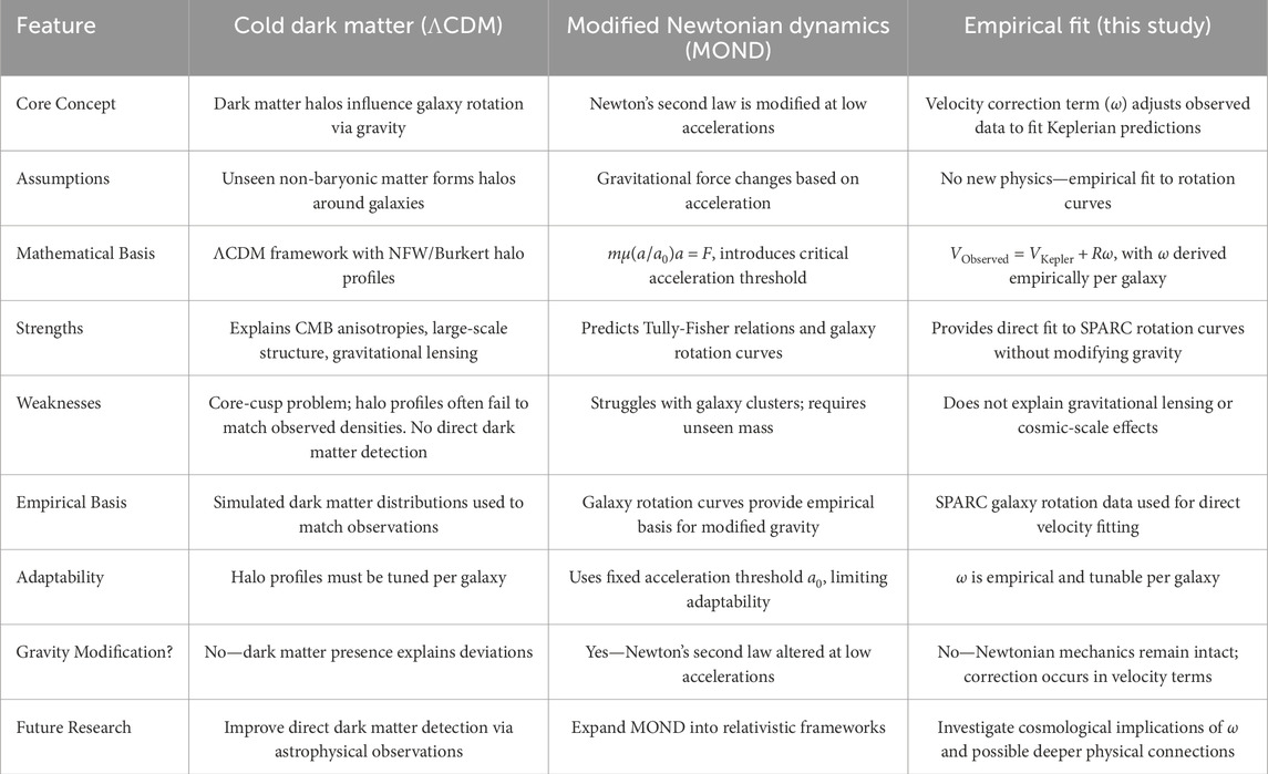
Table 3. Comparison of Cold dark matter ($\mathrm{\Lambda }$CDM), modified Newtonian dynamics (MOND), and empirical fit model.

7 Conclusion

The empirical model’s performance is quantitatively validated in Supplementary Appendix B, where rotation curve fits are compared head-to-head with MOND and CDM models across multiple galaxies.

• Of the 84 galaxies tested, $\omega$ values were found to fall between 1.97 and 15.35 km/sec. In each case, an $\omega$ could always be found to correct the observed stellar velocities back to those predicted by Kepler.

• HI radius has an correlation coefficient of $R^2$ = 0.54 with ${\omega }_{\mathit{eps}}$.

• HI mass has an correlation coefficient of $R^2$ = 0.47 with ${\omega }_{\mathit{eps}}$.

• The survey yielded an $\omega$ Statistical Mean of 7.06 and a Standard Deviation of 3.26 over 84 galaxies.

• The resemblance between Figures 2, 3 for M33 is striking. Figure 4 is a partial data dump of the curves for the first 20 of our 84 galaxies surveyed which all were a very good fit for this method. Figures 5–8 show head-to-head comparisons of our Figure 4 curves (top) to SPARC calculations (bottom) that are also impressively similar using a completely different approach for calculation. We noticed that the $\omega$ correction factor was always within one order of magnitude (statistical mean of 7.06).

Data availability statement

The original contributions presented in the study are included in the article/Supplementary Material, further inquiries can be directed to the corresponding author.

Author contributions

DF: Conceptualization, Formal Analysis, Investigation, Methodology, Project administration, Supervision, Validation, Visualization, Writing – original draft, Writing – review and editing. JC: Data curation, Software, Writing – review and editing.

Funding

The author(s) declare that no financial support was received for the research and/or publication of this article.

Acknowledgements

We gratefully acknowledge Robert Scherrer of Vanderbilt University for his guidance throughout this effort. We also thank Brian Riely for his contributions to statistical interpretation and graphical modeling. Figures 1, 2, Supplementary Appendix Figures 14, 15 were created by our visual artist, Katherine Flynn.

Conflict of interest

The authors declare that the research was conducted in the absence of any commercial or financial relationships that could be construed as a potential conflict of interest.

Generative AI statement

The author(s) declare that Generative AI was used in the creation of this manuscript. Generative AI (Microsoft Copilot) was used to assist with structural refinement and scientific phrasing throughout the manuscript. Specific contributions include: - Suggestions and refinements to the Abstract - Drafting of Section 1.1 (“Comparisons with ΛCDM and MOND”) - Assistance in defining ω and refining Table 3 language (Section 6) - Support for bitmap comparison calculations in Appendix B and B.1 All modeling, analysis, and scientific conclusions were authored and verified by the submitting author. The process improved clarity, reproducibility, and editorial precision without altering the empirical findings.

Any alternative text (alt text) provided alongside figures in this article has been generated by Frontiers with the support of artificial intelligence and reasonable efforts have been made to ensure accuracy, including review by the authors wherever possible. If you identify any issues, please contact us.

Publisher’s note

All claims expressed in this article are solely those of the authors and do not necessarily represent those of their affiliated organizations, or those of the publisher, the editors and the reviewers. Any product that may be evaluated in this article, or claim that may be made by its manufacturer, is not guaranteed or endorsed by the publisher.

Supplementary material

The Supplementary Material for this article can be found online at: https://www.frontiersin.org/articles/10.3389/fspas.2025.1680387/full#supplementary-material

Footnotes

¹Throughout this paper, we use the term “rotation curve” in its observational context—referring to measured velocity profiles as a function of radius, typically derived from Doppler shift data (e.g., HI or stellar spectral lines). While sometimes used interchangeably with “circular speed,” we do not claim that all measured velocities represent perfectly circular orbital motion.

¹Throughout this work, $\omega$ and ${\omega }_{\mathit{eps}}$ are used interchangeably to represent angular velocity estimates derived from distinct but functionally equivalent approximations. Unless otherwise specified, their usage is intended to convey observational parity rather than a strict mathematical identity

¹The terms “closest” and “farthest” star are not used here as absolute measurements, but rather indicate selections based on the most reliable available distance data.

References

Bardeen, J. M., and Petterson, J. A. (1975). The lense-thirring effect and accretion disks around kerr black holes. Astrophysical J. 195, L65–L67. doi:10.1086/181711

CrossRef Full Text | Google Scholar

Benaissa, B. (2025). Resolving galactic rotation curve discrepancies through a proposed relativistic observation effect. SSRN Electron. J. doi:10.22541/au.174189026.62416989/v1

CrossRef Full Text | Google Scholar

Bertone, G., and Hooper, D. (2016). A history of dark matter. Available online at: https://arxiv.org/pdf/1605.04909.

Google Scholar

Chan, M. H. (2022). Two mysterious universal dark matter–baryon relations in galaxies and galaxy clusters. Phys. Dark Universe 38, 101142. doi:10.1016/j.dark.2022.101142

CrossRef Full Text | Google Scholar

Clowe, D., Bradač, M., Gonzalez, A. H., Markevitch, M., Randall, S. W., Jones, C., et al. (2006). A direct empirical proof of the existence of dark matter. Astrophysical J. 648, L109–L113. doi:10.1086/508162

CrossRef Full Text | Google Scholar

Corbelli, E., and Salucci, P. (1999). The extended rotation curve and the dark matter halo of M33. Mon. Notices R. Astronomical Soc. 311, 441–447. doi:10.1046/j.1365-8711.2000.03075.x

CrossRef Full Text | Google Scholar

Corbelli, E., Thilker, D., Zibetti, S., Giovanardi, C., and Salucci, P. (2014). Dynamical signatures of a ΛCDM-halo and the distribution of the baryons in M33. Astronomy and Astrophysics 572, A23. doi:10.1051/0004-6361/201424033

CrossRef Full Text | Google Scholar

de Blok, W. J. G., Walter, F., Brinks, E., Trachternach, C., Oh, S. H., and Kennicutt, R. C. (2008). High-resolution rotation curves and galaxy mass models from THINGS. Astronomical J. 136 (6), 2648–2719. doi:10.1088/0004-6256/136/6/2648

CrossRef Full Text | Google Scholar

Famaey, B., and McGaugh, S. S. (2012). Modified newtonian dynamics (MOND): observational phenomenology and relativistic extensions. Living Rev. Relativ. 15 (10), 10. doi:10.12942/lrr-2012-10

PubMed Abstract | CrossRef Full Text | Google Scholar

Gentile, G., Famaey, B., and de Blok, W. J. G. (2011). THINGS about MOND. Astronomy and Astrophysics 527, A76. doi:10.1051/0004-6361/201015283

CrossRef Full Text | Google Scholar

Katz, H., Lelli, F., McGaugh, S. S., Di Cintio, A., Brook, C. B., and Schombert, J. M. (2017). Testing feedback-modified dark matter haloes with galaxy rotation curves: estimation of halo parameters and consistency with ΛCDM scaling relations. Mon. Notices R. Astronomical Soc. 466 (2), 1648–1668. doi:10.1093/mnras/stw3101

CrossRef Full Text | Google Scholar

Lelli, F., McGaugh, S. S., and Schombert, J. M. (2016). SPARC: mass models for 175 disk galaxies with spitzer photometry and accurate rotation curves. Astronomical J. 152 (6), 157. doi:10.3847/0004-6256/152/6/157

CrossRef Full Text | Google Scholar

Lin, W., and Chen, D. M. (2021). Comparison of modeling SPARC spiral galaxies’ rotation curves: halo models vs. MOND. Res. Astronomy Astrophysics 21 (11), 271. doi:10.1088/1674-4527/21/11/271

CrossRef Full Text | Google Scholar

Lovas, S. (2022). Linearity: galaxy formation encounters an unanticipated empirical relation. Mon. Notices R. Astronomical Soc., Letters. doi:10.48550/arXiv.2206.11431

CrossRef Full Text | Google Scholar

McGaugh, S. S., Lelli, F., and Schombert, J. M. (2016). Radial acceleration relation in rotationally supported galaxies. Phys. Rev. Lett. 117 (20), 201101. doi:10.1103/physrevlett.117.201101

PubMed Abstract | CrossRef Full Text | Google Scholar

Milgrom, M. (1983). A modification of the Newtonian dynamics as a possible alternative to the hidden mass hypothesis. Astrophysical J. 270, 365–370. doi:10.1086/161130

CrossRef Full Text | Google Scholar

Rubin, V. C. (2011). An interesting voyage. Annu. Rev. Astronomy Astrophysics 49, 1–28. doi:10.1146/annurev-astro-081710-102545

CrossRef Full Text | Google Scholar

Sanders, R. H., and McGaugh, S. S. (2002). Modified newtonian dynamics as an alternative to dark matter. Annu. Rev. Astronomy Astrophysics 40, 263–317. doi:10.1146/annurev.astro.40.060401.093923

CrossRef Full Text | Google Scholar