Including predation risk in mechanistic habitat assessment models for stream fish

Mechanistic habitat assessment models have long been used for stream fish, especially drift-feeding salmonids. Most of these models assess habitat value as the rate of net energy intake (growth) obtained by a fish feeding in a habitat unit. However, the fitness value of habitat and the willingness of fish to occupy it also depend on predation risk: habitat is not valuable if it offers high growth but also high risk. Methods for modeling how predation risk varies with characteristics of habitat and fish are much less developed than those for modeling net energy intake. We present approaches we use in InSTREAM, an individual-based salmonid population model, to represent how risk from several kinds of predation depend on fish characteristics (size, activity) and habitat characteristics including depth, velocity, availability of escape and concealment cover, temperature, light intensity, and turbidity. Such models of risk are by nature complex, but they can be designed and parameterized using a variety of conceptual models, literature, and field experiments. Incorporating risk in habitat assessment models also requires combining simulated growth and risk into a meaningful measure of the overall fitness value of habitat. We present a measure of expected future survival of both predation and starvation as a practical, proven measure of fitness value. Assessing habitat explicitly as a measure of future fitness provides conceptual clarity to models, for example by identifying habitat variables more meaningful than some traditional measures (e.g., distance to escape cover instead of generic cover availability) and by illuminating differences between predation by fish and by terrestrial animals. But explicitly considering fitness also highlights the conceptual limitations of habitat-only models for management decision support. In contrast, individual-based population models like InSTREAM provide a way to make meaningful and testable predictions of the effects of habitat change on fish populations.

1 Introduction

Mechanistic fish habitat assessment models evaluate particular habitat types for particular types of fish, by representing how a specific measure of individual fitness depends on characteristics of both habitat and fish. These models have long been developed and used for drift feeders—fish, especially salmonids, that feed by maintaining a fixed position and capturing food particles carried past by the stream current. Classic drift-feeding models represent: (a) net energy intake (NEI; the difference between the rate of energy gain from food capture and the rate of energy expenditure for basal and swimming metabolism, assumed proportional to growth) as the measure of fitness provided by habitat; (b) water depth and velocity as the habitat characteristics affecting NEI; and (c) length and weight as fish characteristics affecting NEI. These models assume that, as water velocity increases the rate of food delivery to the fish increases, its ability to capture food decreases, and its metabolic costs increase. Consequently, NEI and growth peak at an intermediate velocity that increases with the size of the fish. Grossman (2014); Piccolo et al. (2014), and Rosenfeld et al. (2014) review NEI and related models. Naman et al. (2020) developed their use as a habitat evaluation approach for drift feeders, specifically as an alternative to the empirical relations between hydraulic variables and fish occupancy used in traditional habitat assessment methods such as PHABSIM (Bovee et al., 1998).

The fundamental assumption of NEI models, when used to assess habitat, is that fish select habitat to maximize their growth rate; yet a variety of observations indicate that stream fish can be highly concerned with predation risk. Therefore, when microhabitat-resolution individual-based models appeared as a way to evaluate stream habitat and management effects on trout populations, they attempted to represent habitat selection as depending on both growth and predation risk (e.g., Van Winkle et al., 1998). The methods used to represent risk and its effects on habitat selection in our InSTREAM individual-based trout model (Railsback et al., 2021a, 2023) contribute to the model reproducing a wide range of observed salmonid behaviors (Railsback and Harvey, 2002; Railsback et al., 2005, 2020).

InSTREAM simulates stream habitat and the trout that occupy it. It represents habitat as microhabitat cells with (a) depths and velocities that depend on stream flow, and (b) static variables for availability of velocity shelter that reduces swimming costs for drift feeders, and predation avoidance cover. On each time step, simulated fish select a habitat cell by considering how their growth and survival probability depend on both cell habitat and competition with any larger fish occupying a cell.

Our objectives here are to discuss why and how predation risk can be represented in mechanistic habitat assessment models, whether those models address only habitat (e.g., Naman et al., 2020) or also individuals and populations (as InSTREAM does). First, we provide evidence that risk affects fish habitat selection and survival in ways that can strongly affect conclusions drawn from management models. Second, we discuss conceptual models of how predation risk varies with characteristics of habitat and the prey fish. Third, we present ways of representing habitat effects on risk: what variables are useful, how risk is usually related to those variables, and how we can observe those relationships in the field. Next, we discuss ways that risk and growth can be combined into meaningful mathematical measures of individual fitness appropriate for evaluating habitat, and why some common approaches do not work. We then consider the potential use of such fitness measures by themselves as a habitat assessment method, e.g., as replacements for suitability criteria in PHABSIM (e.g. Naman et al., 2020). Unfortunately, including predation risk emphasizes instead of reduces many of the inherent uncertainties in habitat suitability models.

Because our models—like most NEI models intended for management applications—address stream salmonids, we refer to the modeled fish as trout. We refer to habitat as cells that have variables such as depth, velocity, and cover availability that differ among cells and change over time. “Risk” refers specifically to predation risk unless otherwise noted. When used mathematically, we express risk as probability per day of mortality, and “survival” is the daily probability of surviving (1 – risk).

2 Is risk important?

Over recent decades, a great deal of ecological literature has addressed the importance of predation risk on animal behavior and population dynamics (e.g., Brown et al., 1999; Preisser et al., 2005). Is it important to consider predation risk in mechanistic models of habitat benefits to trout, or is it sufficient to only consider growth? One way to answer this question is via empirical experimentation to see if risk prevents fish from using habitat that provides high growth. Harvey and White (2017) conducted exactly such an experiment: they offered juvenile salmonids high rates of food intake in habitats that were increasingly risky due to lower depths and higher distances to escape cover. They observed that fish would use riskier habitat only if it provided more food, and fish would not use the riskiest habitat (e.g., depth <20 cm) no matter how much food was provided. This evidence aligns with a variety of previous studies that indicate stream fish consider both food acquisition and risk when selecting habitat (e.g., Gilliam and Fraser, 1987; Grand and Dill, 1997; Naman et al., 2019).

However, evidence that risk affects fish habitat selection does not necessarily mean we need to consider risk in management analyses such as the evaluation of alternative instream flow regimes. Do models that only address growth produce results similar to those of models that also consider predation risk, such that the two kinds of models might lead to the same management conclusions? We addressed this question in two ways, using the InSTREAM version (7.0) and application sites of Railsback et al. (2021b). The two sites are a habitat restoration site with complex and diverse habitat, and a degraded site with a simple, U-shaped channel (Figure 1). First, we contrasted two measures of habitat availability: the percentage of stream area providing positive growth for a 15-cm trout at 15°C and negligible turbidity, and the percentage of stream area that provides positive growth and daily survival probability > 0.99 (Figure 2). Second, we examined the importance of considering risk by simulating how long-term populations varied across a range of flow regimes (the same range examined by Railsback et al., 2021b), using (a) InSTREAM’s standard formulation in which risk varies with characteristics of both habitat and individual fish, and (b) uniform risk, with all fish subject to the same daily predation survival probability of 0.995 (Figure 3).

Figure 1

Figure 1. The restored (top) and degraded (bottom) sites, with cells shaded by depth at a simulated flow of 5.0 m³/s. The sites are displayed at the same scale; the degraded site extends 1350 m from left to right.

Figure 2

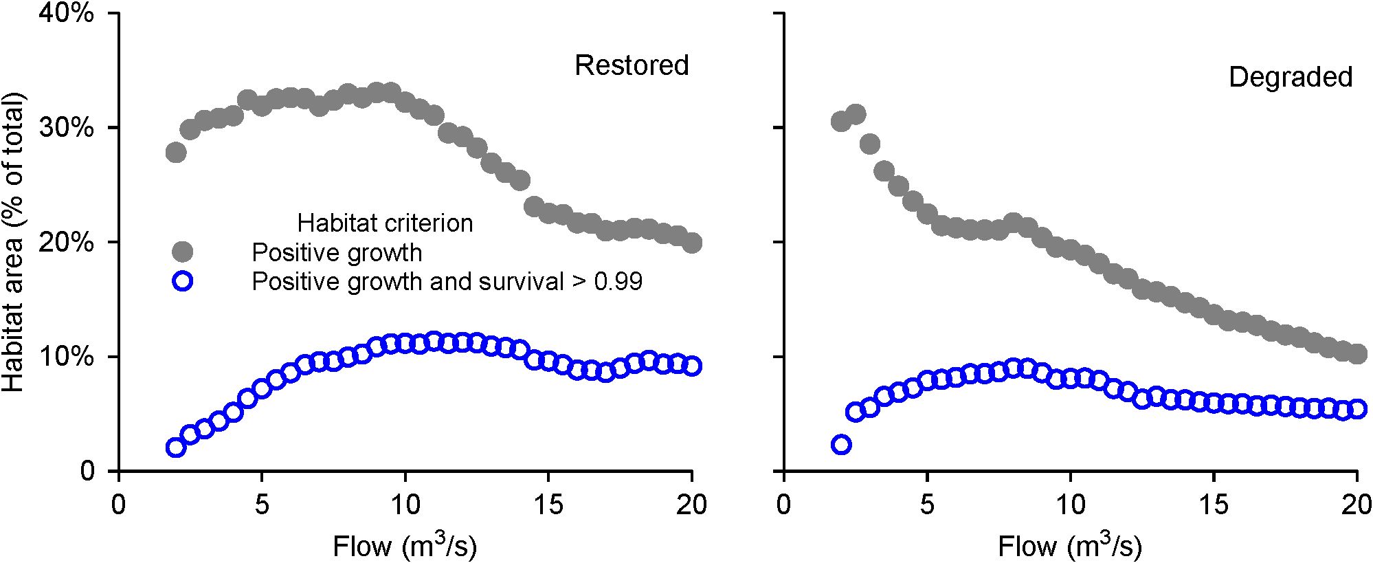
Figure 2. Predation risk affects how area of usable habitat varies with flow in simulated stream reaches. Habitat area is the percentage of total stream area providing positive growth (filled symbols) or positive growth and daily survival > 0.99 (open symbols), for a 15-cm trout at 15°C. Daily survival of 0.99 corresponds to 74% survival per month. Input and parameter values are from Railsback et al. (2021b).

Figure 3

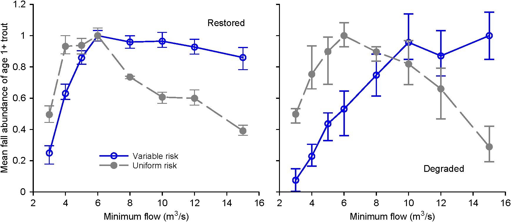
Figure 3. Representing variation in risk affects predicted population responses to instream flow. The Y axis is the predicted abundance of adult trout (mean abundance on September 30^th of simulated years 2004-2011), expressed as the fraction of maximum mean abundance across all flow scenarios. Minimum flow scenarios range from 3 to 15 m³/s. Open symbols indicate results with risk that varies among fish and habitat cells, and closed symbols indicate uniform risk. Simulations were otherwise identical to the “4-phase” simulations illustrated in Figure 2 of Railsback et al. (2021b). Symbols and error bars represent the mean, minimum, and maximum values over five replicate simulations.

Both of these approaches show that including how risk varies with habitat and among fish strongly alters the relation between instream flow and predicted habitat benefits, particularly by predicting greater benefits of higher flows. The effects are especially clear at the degraded site, where the simple channel provides, at low flows, ample habitat for growth but little protection from predation. Consequently, the population simulations considering NEI only predict highest abundance at a lower range of flows than do the simulations with non-uniform risk. This simple experiment indicates that evaluating habitat via NEI only and ignoring risk is likely to result in instream flow analyses that—for at least some channels—favor conditions that real trout would be afraid to use.

3 Conceptual models of predation risk to stream fish

We begin our discussion of predation risk in habitat evaluation models by identifying conceptual models of how risk varies that we have found useful and well-supported. These conceptual models are generalizations about how risk varies with characteristics of habitat, predators, and trout prey; they of course have many exceptions.

3.1 Terrestrial predators and fish predators are different

Stream trout are at risk from other fish, and also from a wide variety of terrestrial animals (Alexander, 1979; Harvey and Nakamoto, 2013). Key terrestrial predators include diving birds (e.g., mergansers, cormorants), wading birds, raptors, otters and other mustelids, and snakes. Even where trout are the only fish, predation by larger trout on smaller can be a major source of mortality. Following Power (1987) and Harvey and Stewart (1991), we have found it useful to consider risk from terrestrial and fish predators separately: these two categories have strong general differences in how risk varies, especially with three important variables. Treating multiple categories of predators as separate risks does not substantially increase model complexity: survival probabilities can be modeled separately for each category and then multiplied together to determine survival of all categories.

Fish size: Throughout ecology, the assumption that risk decreases as prey grow is a common conceptual model. This conceptual model seems valid for fish predation on trout: the risk of being consumed by another fish decreases as juveniles grow, due to predator gape limitation and increasing ability of prey to detect and evade predators. (However, Harvey, 1991 and Layman and Winemiller, 2004 provide evidence of larger fish predators being more responsive to larger prey.) The relation between trout size and risk of fish predation can depend very much on what fish prey on them: the size at which juveniles become relatively safe depends on whether they are at risk only from relatively small adult trout, from large adults (e.g., in large rivers; Meyer et al., 2003), or from large-gaped warmwater piscivores (e.g., bass, pikeminnow; Michel et al., 2020). In contrast to risk from fish predators, risk from many terrestrial predators likely increases with prey size, with the possible exception of unusually large individuals. Small juveniles may be at less risk because they are harder to see from above and less profitable.

Depth: Increased depth appears to give fish some protection from terrestrial predators, especially wading birds and those that depend on seeing prey from above (Power, 1984; Harvey and White, 2017). Just the opposite is true for fish predators: large fish are vulnerable to terrestrial predators in shallow water and avoid it, making small fish safer from fish predation in shallow water (e.g., Rypel et al., 2007). The combined effect of increasing effectiveness of terrestrial predators with decreasing depth and increasing effectiveness of fish predators with increasing depth suggests that the safest depth increases with prey fish size (Power, 1987; Harvey and Stewart, 1991).

Temperature: Predation rates by fish are commonly assumed to be reduced at low temperatures, because fish metabolic and digestion rates are low at low temperatures. In contrast, terrestrial predators (except reptiles) are endothermic and, if anything, need more food in cold weather; Harvey and Nakamoto (2013) observed higher risk in winter-spring than in summer. However, bird migration, mammal hibernation, and ice cover may reduce terrestrial predation on fish in winter.

3.2 Risk is largely, but not entirely, driven by vision

Most, if not all, predators depend largely on vision to identify and capture prey fish, so it is reasonable to assume that risk is lower under conditions that make fish prey less visible. Overhead predators such as birds must see fish through the water surface, so risk can be reduced by depth and hydraulic conditions that induce water surface complexity and distortion in surface refraction. Elevated turbidity substantially reduces fish visibility and enhances the benefits of depth. However, risk from predators that identify prey under water (fish, otters) likely varies less with visibility: conditions that make prey harder to see also make predators harder to detect and avoid, and larger predators typically have better vision.

3.3 Risk varies among times of day

Because risk is largely driven by vision, it can vary dramatically among times of day when light levels are high (day), reduced (dawn and dusk), and low (night). This variation is, along with dependence of feeding success on light (e.g. Fraser and Metcalfe, 1997), among the reasons that we need to consider day, crepuscular periods, and night separately when evaluating habitat (Railsback et al., 2021b). Reduced risk from terrestrial predators is presumably a primary explanation for observations (Valdimarsson and Metcalfe, 1999; Jakober et al., 2000; Harwood et al., 2001) of salmonids using shallower depths at night and feeding often during crepuscular periods (Johnson et al., 2016). However, some predators are effective at night; over 1/3 of predator encounters observed by Harvey and Nakamoto (2013) were at night by owls, otters, and raccoons.

3.4 Risk—and what affects it—varies with fish activity

Risk is important to habitat evaluation not only because it affects where fish choose to feed but also because it affects when they choose to feed. Observations such as those of Metcalfe et al. (1998, 1999) and Valdimarsson and Metcalfe (1999) indicate that salmonids reduce risk by concealing themselves in substrates at times of day when they can afford to not feed. The many implications of these tradeoff behaviors include that: (a) habitat effects on risk are presumably less important for fish that are concealing than for those feeding, and therefore (b) habitat evaluation—for both feeding and risk—is most meaningful when focused on the times of day when most fish are feeding; but (c) the availability of concealment habitat is important and potentially could affect behavior and risk (Armstrong and Griffiths, 2001; Harwood et al., 2002). Railsback et al. (2021b) discuss such implications and explore their consequences.

3.5 Some risks can be episodic

The methods and models we consider here treat predation risk as a steady threat, except for effects of seasonal changes in temperature and light availability. However, our field experience provides anecdotal evidence that predation can also occur as severe, short-term episodes inflicted by highly effective predators. For example, dry-season survival of trout in field experiments at one study site varied strongly between years (Harvey et al., 2005, 2006); we observed abundant otter scat, which included PIT tags from trout, only in the year with relatively low fish survival. Such episodes cannot be predicted reliably with models, and the predators responsible are probably effective under most conditions. We do not attempt to model episodic predation, but it can be considered in field studies and attempts to parameterize or test models against field observations.

4 Effects of habitat and prey fish characteristics on predation risk

For spatially explicit modeling, the challenge of including predation risk requires estimates of predation risk for individuals within the habitat units included in the model, with risk depending on multiple characteristics of both habitat and fish. In the InSTREAM model, we use “survival increase functions” to represent how separate characteristics of habitat cells and individual prey fish affect risk (Figure 4). These are functions (often, logistic curves) that describe how one habitat or prey variable affects survival probability; they range from 0 (no reduction in risk) to 1 (complete protection). These functions are treated as general relations that are each based on a variety of evidence, and that need little or no adjustment among model application sites.

Figure 4

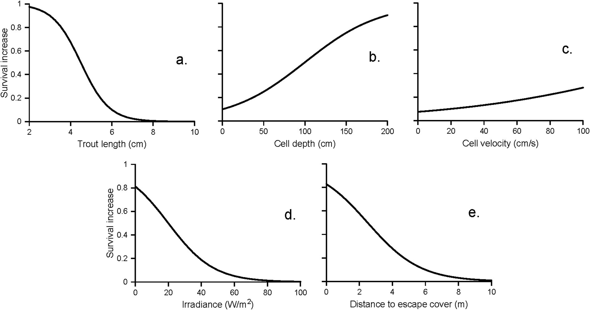
Figure 4. Example survival increase functions for terrestrial predation on trout in a small stream. Survival is assumed highest for (a) smaller trout, (b) deeper water, (c) faster water (but the effect is small), (d) low light intensity (irradiance is typically > 200 during daylight, < 20 during dawn and dusk, and < 1 at night), and (e) lower distance to escape cover.

The first step in our process of modeling risk is to determine what habitat and prey characteristics to include in the model and how to quantify them in ways most directly related to predation risk. Traditional measures of salmonid habitat such as substrate size or the amount of wood within habitat units may not best describe variation in predation risk. In InSTREAM, we use a representative distance to escape cover as the variable to describe the availability of cover relevant to immediate avoidance of predation, without regard for the material providing the cover (e.g. stone substrate, undercut banks, or vegetation). The availability of cover useful for long-term concealment behavior is treated separately. InSTREAM includes habitat depth as a factor affecting risk, although it is assumed to have opposing effects on predation risk from aquatic versus terrestrial predators. InSTREAM also includes water velocity as a potential reducer of risk from terrestrial predators. Both water velocity per se and the surface turbulence commonly associated with water velocity in streams may reduce visibility from overhead and therefore risk from terrestrial predators. We believe meaningful relations between risk and factors such as cover, depth and velocity can be established at the scale of habitat units typically used in InSTREAM (2–20 m² area), but these are unlikely to be directly usable in models that represent habitat on larger spatial scales. In contrast, other risk-affecting factors such as temperature and turbidity may be readily represented on larger spatial scales.

While neglected in InSTREAM, effects of prey fish density on risk could be represented in models. Within some specific spatial resolution, higher prey density could be assumed to reduce per-individual risk (especially for schooling fish) due to prey dilution and enhanced prey detection, or to increase risk by attracting predators.

The second step in our risk modeling process is to develop quantitative survival increase functions such as those in Figure 4. Formulation of functions relating predation risk to habitat and prey fish characteristics will almost always involve substantial speculation: few available observations can serve directly as data points. Modelers can overcome this limitation in several ways. First, functions relating risk to habitat or fish characteristics can be based on the kinds of conceptual models discussed above. For example, a relation between prey fish length and the risk of predation by other fish can be based on the “gape limitation” concept: as a fish grows, fewer other fish are large enough to consume it. Likewise, it makes conceptual sense that a fish’s risk of capture increases with its distance from escape cover. Relations based on conceptual models can often be supported and quantified by empirical evidence from the literature. Where piscivorous warmwater fish are a significant risk, for example, the conceptual model that risk increases with temperature as their metabolic rates increase can be supported with laboratory data on how piscivore respiration and digestion rates vary with temperature.

A second way to address uncertainty in risk relations is via empirical evidence. Traditional ecological field experiments can provide direct measures of relative predation risk, with the caveats that enclosure effects may vary among treatments and many experimental units will be needed to provide the range of treatments necessary to achieve the goal of describing complete gradients in risk. Tethering experiments can also provide direct measures of risk, but these also must be interpreted with caution, in part because of the potential for unequal tethering artefacts across treatments (Baker and Waltham, 2020). Combining tethering with camera trapping (Harvey and Nakamoto, 2013) mitigates the problem of prey losses not due to predation and adds information on predator identity.

A variety of indirect measures of risk may inform the effort to quantify habitat – risk relations. While fundamental risk and the perception of risk cannot be strictly equated (Gaynor et al., 2019), the latter may provide useful information for the purpose of quantifying habitat – risk relations. Harvey and White (2017) measured giving-up harvest rate with a purpose-built feeding device to quantify the perception of risk in stream salmonids along gradients of water depth and distance to cover. This approach seems likely to have limited application due to a variety of constraints, including the need to train individual fish to use a feeding device and the likely confounding influence of a variety of nuisance variable such as fish condition and the availability of alternative food resources in natural settings. Giving up food density, successfully used to measure the perception of risk in a variety of prey taxa (Gaynor et al., 2019), is likely to be difficult to apply in efforts to measure the perception of risk on relatively small spatial scales for many stream fishes, because of their ability to capture static food resources in brief forays to risky areas. Observations of where predation occurs have been widely used to assess predation risk in other systems (e.g. ungulate-carnivore, [Miller, 2015]), but such observations are more difficult in aquatic systems, in part because evidence of kill sites does not persist. However, camera trapping has been used to quantify predation rates on unconfined stream salmonids (Sullivan et al., 2023). Importantly, passive observations measure realized predation rather than fundamental predation risk: predation events are affected by antecedent habitat selection of prey and predators. Also, prey density affects per capita risk. Passive observation of predator presence alone, although an additional step away from fundamental predation risk, might also provide useful information for the purpose of estimating habitat – risk relations.

A third way to address uncertainty is via model analysis: once a model has been applied to a site, it can be analyzed to determine (e.g.) how sensitive model results are to parameters controlling each risk relationship and how sensitive management decisions based on model results (often, the rank of management alternatives such as instream flow regimes) are to uncertainty in parameter values. Such analyses are especially valuable if they guide field studies to better understand especially important relations; the study by Harvey and White (2017) was inspired by a parameter sensitivity analysis of an early version of InSTREAM that showed the relation between water depth and risk from terrestrial predators to be especially important.

The survival increase functions for terrestrial predators in Figure 4 were developed using all these methods (Railsback et al., 2023 provide full details). The function for trout length is based on the conceptual model that very small prey fish are difficult to see, can readily hide in most substrate, and are of little value to predators. The function for cell depth is based on the conceptual model that increasing depth reduces visibility to overhead predators, supported by the field observations by Harvey and White (2017) of trout willingness to feed vs. depth. The function for cell velocity is based on the concept that surface turbulence, which often increases with velocity, reduces visibility from overhead. The irradiance (light intensity) function is based on knowledge of irradiance values at different times of day, and on the assumption that most terrestrial predators are less effective at low light levels but night predation is still common. The escape cover function is based on the conceptual model that the time it takes a prey fish to reach nearby escape cover is approximately inversely proportional to its distance from cover, while distant cover offers little protection.

5 Incorporating risk in habitat evaluation metrics

Once we have determined how to represent the separate effects on predation risk of several different characteristics of habitat and a fish, how do we combine those effects into one estimate of survival probability? And then how do we consider that probability in a meaningful measure of habitat value? We consider these questions here.

5.1 Combining effects of multiple habitat and fish variables

Section 4 considers survival increase functions that representing how habitat and fish variables affect survival probability. Here, we present two methods for combining these functions into a single value of survival probability for one type of predator; InSTREAM uses these methods to determine separate probabilities of surviving terrestrial and fish predators.

Both methods use a parameter that represents a minimum daily survival probability (S_min), essentially the survival probability for fish under the riskiest conditions, and then determine survival S for a particular fish at a particular habitat cell and time by using the survival increase functions to modify S_min.

The first method (used in early versions of InSTREAM; Railsback et al., 2009) simply assumes that only the function providing highest survival increase affects S. The value of S is determined by adjusting S_min to reduce risk by the highest value of the survival increase functions (F_max):

$\begin{array}{ll}S=S_{min}+(1-S_{min})F_{max}& (1)\end{array}$

For example, consider a trout with: (a) length of 5 cm and therefore (using the functions illustrated in Figure 4) a length survival increase function value of 0.32; (b) cell depth of 20 cm, so a depth survival increase of 0.15; (c) velocity of 15 cm/s, with velocity survival increase of 0.09; (d) daytime irradiance of 350 W/m², providing zero survival increase; and (e) distance to escape cover of 3 m, so survival increase of 0.42. In this case, the highest survival increase (F_max = 0.42) is provided by distance to escape cover. If S_min is 0.95, then Equation 1 produces S = 0.971. (The maximum daily risk corresponding to S_min = 0.95 is 0.05. Reducing that risk by 42% gives an adjusted risk of 0.05×0.58 = 0.029, so S = 1.0–0.029 = 0.971).

The second method is used in current versions of InSTREAM (Railsback et al., 2023; see also Railsback and Harvey, 2025). It considers that each habitat variable with a survival increase function can contribute to reducing risk, so survival depends on all such variables. We model the interaction among survival increase functions (F_i where i indicates the functions, e.g., from a to e in Figure 4) by treating each F_i as a survival probability and calculating the probability of not surviving all of them:

$\begin{array}{ll}S=S_{min}+(1-S_{min})(1-{\displaystyle {\prod }_{i=1}^{i=n}(1-F_i)})& (2)\end{array}$

Using the above example trout, the product term in Equation 2 is: (1–0.32)(1–0.15)(1–0.09)(1–0.0)(1–0.42) = 0.302, and S = 0.985. Using this method, all the survival increase functions affect S but S is most sensitive to the functions with highest values.

Neither of these approaches represents interactions among the ecological factors affecting risk, even though such interactions (e.g., the benefit of depth increasing as light intensity decreases or turbidity increases) are likely. Such interactions could of course be added to a model, if the benefits of additional realism appear to outweigh the costs of additional model complexity.

5.2 Combining survival and growth into a measure of habitat value

Once we have predicted NEI or growth rate (g, grams biomass accumulation per day) for a particular fish in a particular habitat cell, and used methods such as the above to predict S for several categories of predators, how do we combine them into a meaningful measure of habitat value? This question is the subject of extensive literature in behavioral ecology. Here, we briefly summarize relevant theory from behavioral ecology and its concepts relevant to evaluating fish habitat, but also show why little of that theory is directly applicable to the fish habitat assessment problem. The points discussed here are considered extensively by Railsback and Harvey (2020).

The basic concept of much behavioral ecology, including optimal foraging theory, is that animals use behaviors—such as selection of habitat cells—to maximize their expected fitness, where fitness involves future reproductive success. Future reproductive success requires survival—of predation, starvation, and other risks—to a future reproductive cycle, and accumulation of the size and energy reserves needed to produce offspring. To evaluate habitat, we need a “fitness measure” that represents how a cell affects at least some of these elements of fitness. We could attempt to use a fitness measure that explicitly represents a fish’s expected future reproductive output if it occupied the cell, but doing so would require complex calculations and a number of highly uncertain assumptions (considered below in Sect. 6). Instead, we need a relatively simple, computationally tractable fitness measure that still captures the tradeoff between growth and risk.

The “minimize µ/g rule” has been widely misused as an approximation for trading off growth and risk to maximize future fitness. Gilliam and Fraser (1987) used simplifying assumptions about a very simple foraging system to derive that highest future fitness is provided by the behavior that minimized the ratio of predation risk (µ, = 1–S) to food intake rate. The simplicity of this “rule” is highly appealing and it has been used in a number of models. However, this approach (or any other simple approach based only on S and g) neglects processes often important in more realistic settings (discussed immediately below) and can produce very questionable results in such settings (Railsback et al., 1999).

The “state-based dynamic modeling” theory of behavioral ecology (e.g., Houston and McNamara, 1999; Clark and Mangel, 2000) provides a useful conceptual approach for evaluating risk–growth tradeoffs. Key lessons from that theory and our adaptation of it to fish habitat evaluation (Railsback et al., 1999; Railsback and Harvey, 2020) are:

● The most important elements of fitness are survival to a future time and, for juveniles, attaining reproductive size.

● Survival to a future time must include survival of both predation and starvation. (Here, we use “starvation” to refer to physiological risks, including disease, associated with low body condition.) A fitness measure that considers survival of both predation and starvation ensures that behavior balances avoiding predation and obtaining sufficient food and growth.

● Useful fitness measures must project survival and growth into the future. Doing so is especially important for survival because small changes in daily survival probability result in major differences in long-term survival. A 1% change in S, from 0.99 to 0.98, decreases the probability of surviving for 30 days (S³⁰) from 74% to 55%.

● Survival of starvation can also only be evaluated meaningfully by projecting into the future: a fish in poor condition is unlikely to starve on any particular day but its probability of surviving an extended period is low unless it obtains growth. The risk posed by a particular rate of negative growth depends on a fish’s current size and condition and the time period over which survival is evaluated. For individuals not already starving, a habitat cell that provides a low rate of weight loss might provide a low-enough risk of future starvation to make it temporarily preferable to alternatives offering positive growth but high risk.

● Growth has more fitness value for juveniles than for adults. Juveniles can only reproduce if they grow, but once they reach adulthood further growth is not absolutely necessary for reproduction. (In reality, growth does have fitness benefits for adults: larger size typically results in higher fecundity and ability to compete for mates, and adults must accumulate energy to produce gonads. Those benefits can be included in a fitness measure at the cost of additional complexity; in our experience with InSTREAM, it is not necessary to do so to produce realistic habitat selection and population size distributions).

Despite the usefulness of these concepts, classical state-based dynamic modeling has limitations as a habitat assessment approach in management models. This theory, like most behavioral ecology theory, addresses behavior of one individual in the absence of either interaction with other individuals or unpredictable variation in habitat. It can predict the “optimal” habitat choices of an individual when future conditions are known and unchanging, but there are no optimal choices when future conditions are variable and unpredictable due to either habitat variation (e.g., changes in flow or temperature) or to competition with other individuals also seeking good habitat. Further, state-based dynamic modeling uses complex optimization algorithms that become intractable in many realistic systems. Instead, we must settle for simplified approaches that approximate the fitness value of habitat while still capturing the key effects of habitat and fish characteristics.

InSTREAM assumes individual trout select a combination of habitat cell and activity (feeding vs. concealing) that provides the highest value of a fitness measure that represents expected survival of both predation and starvation over a future time horizon, assuming that both S (daily probability of surviving all predators) and g will remain constant over the time horizon (Sect. 9.13.2 of Railsback et al., 2023). These assumptions that simulated fish use, that they will remain in the same cell and that habitat does not change over the time horizon, are inaccurate but useful: they result in good habitat selection decisions when optimal decisions are not possible (Railsback and Harvey, 2020). We use time horizons of 60–90 days because (a) such lengths are necessary for starvation to become a significant risk, even in unfed fish; and (b) in simulation experiments, lower and higher values produced lower population abundance. For juveniles, the fitness measure includes an additional term representing the benefit of growth, which is assumed to decrease as the fish approaches reproductive size.

This fitness measure is sensitive to both growth and predation risk for juveniles (Figure 5, left panels). For adults in good condition (Figure 5, top right panel) it is sensitive only to risk unless growth is negative: growth is assumed to have no benefit as long as fish maintain their condition. Fish in poor condition (including recently-spawned adults; Figure 5, lower right panel) have fitness sensitive to growth even at positive growth rates: rapid growth lets such fish rapidly reduce starvation risk.

Figure 5

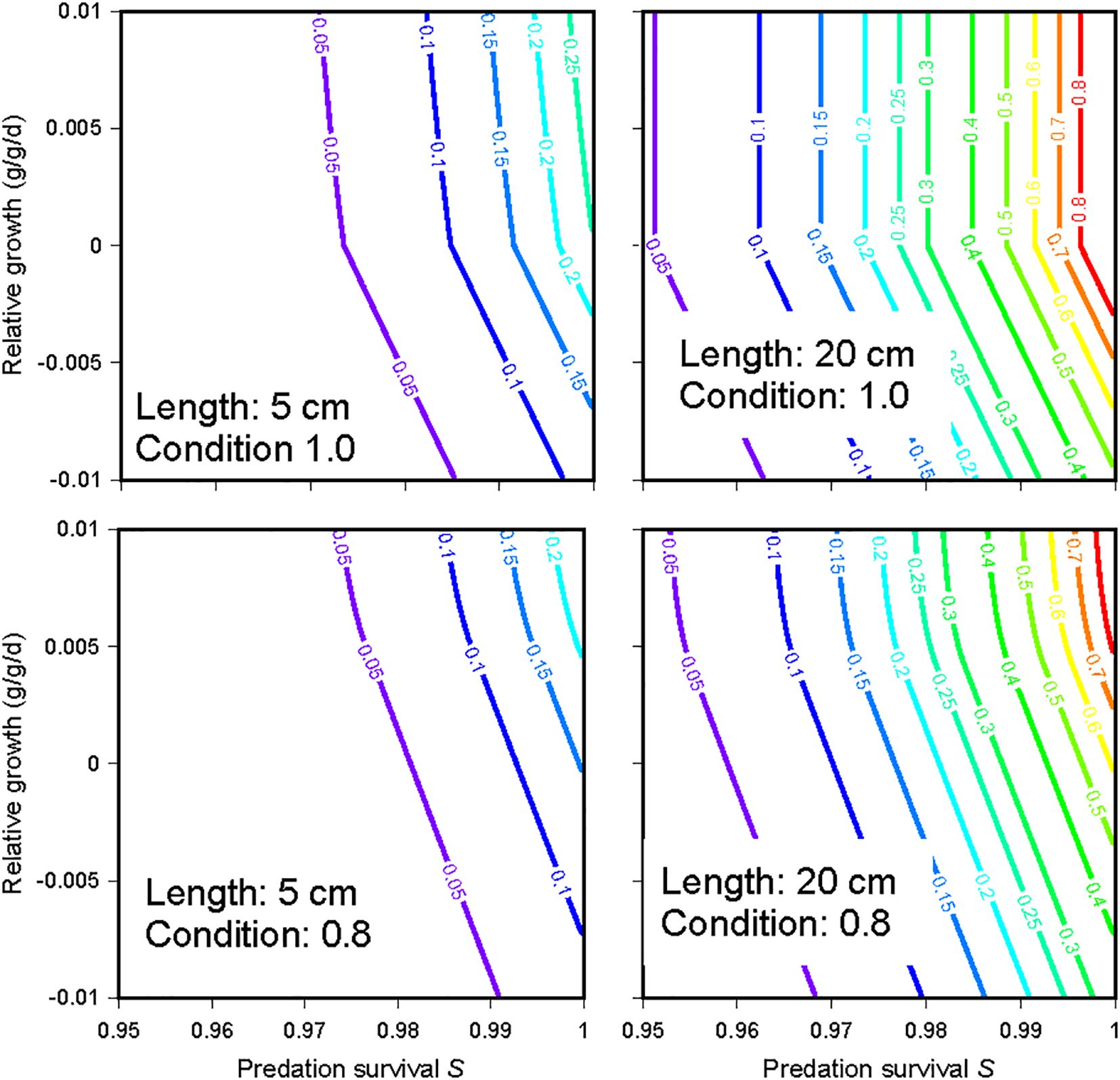
Figure 5. Contours of InSTREAM’s fitness measure over wide ranges of daily predation survival probability S and relative growth (grams biomass accumulation/grams biomass/day). The panels indicate fitness for (left) 5-cm and (right) 20-cm trout with condition (ratio of weight to “healthy” weight) of (top) 1.0 and (bottom) 0.8.

6 What does it mean to fish?

It is tempting to directly apply a fitness measure such as InSTREAM’s as a measure of habitat value. We could assume a typical fish size and condition, and a particular set of habitat conditions—river flow, temperature, turbidity—and then calculate, for example, the area of stream that provides >50% expected probability of the fish surviving predation and starvation for 60 days. Such a habitat measure would certainly have clearer ecological meaning than the habitat “suitability” measure of PHABSIM. (PHABSIM, a widely used management model, evaluates habitat using “suitability” functions that are typically developed from empirical habitat selection data; Bovee et al., 1998. One criticism of PHABSIM is that its suitability functions lack clear biological meaning; Railsback, 2016).

Unfortunately, that approach would still ignore major factors and uncertainties that undermine its meaningfulness. First, the physical and water quality variables that drive growth and survival—flow, temperature, turbidity—inevitably change over time and fish respond to those changes by adapting where and when they feed. Second, the daily light cycle affects growth and survival, and fish adaptively select different habitat and activities at different times of day (discussed by Railsback et al., 2021b). Third, the approach does not address competition: the growth and survival provided to individuals by a habitat cell decreases as the number of fish occupying it increases. Finally, this approach does not eliminate a fundamental limitation of habitat models: even habitat measures with clear meaning for particular individuals (e.g., 4-cm fry, 10-cm juveniles, and 20-cm adults) do not have clear meaning for populations. Meaningful evaluation of alternative instream flow regimes or habitat restoration projects at the population level requires evaluating their cumulative effects across all life stages. Including both growth and predation risk in a measure of habitat value makes these basic limitations of habitat modeling even harder to ignore.

Individual-based models (IBMs) are the only approach we know of that has been used to overcome these limitations. IBMs let us represent how habitat and animals change over time, how animals adapt to those changes and compete, and therefore how life stages are linked over time to produce meaningful and testable predictions of population response to management alternatives. IBMs have the cost of additional assumptions and parameters, but also the advantage of providing a way to estimate particularly important and uncertain parameters. For example, estimating the value of S_min in Equation 2 via field studies is very challenging, but we can readily estimate it (along with food availability) via calibration of an IBM: we can adjust these parameters until the model produces realistic fish abundance and size results. For stream salmonids, InSTREAM and InSALMO (a version of InSTREAM for freshwater lifestages of salmon) are ready-to-use IBMs that have been validated in a number of ways (Railsback et al., 2021a, 2023).

7 Conclusions

Mechanistic habitat assessment models for stream fish have important advantages over traditional observation-based habitat selection approaches (Rosenfeld et al., 2014; Naman et al., 2020). They provide conceptual clarity by representing specific elements of individual fitness, and are more reliable under novel conditions (new sites, different flows, different species mixes) than models based only on observed habitat selection. However, mechanistic approaches that consider growth (or NEI) as the only element of fitness neglect the potentially strong and important effects of predation risk on the value of habitat. Ignoring risk in habitat assessment is likely to over-value habitat that provides high growth but low survival probability because it lacks features such as depth and escape cover that reduce risk (Figure 6). The consequence, as we illustrate in Figures 2 and 3, can be underestimation of the flow needed to provide safe as well as productive habitat.

Figure 6

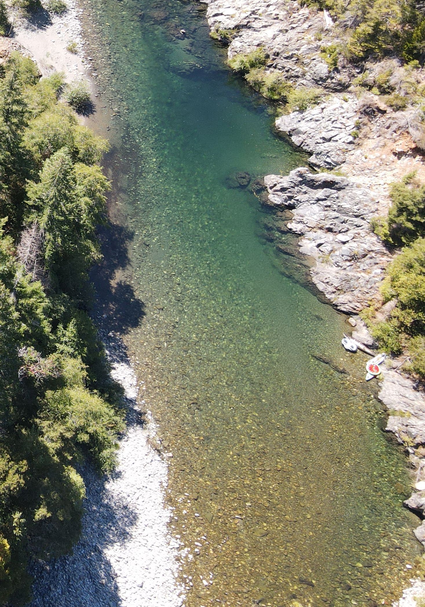
Figure 6. The lower end of this stream reach (S. Fork Smith River, Del Norte County, California) exemplifies habitat providing excellent hydraulic conditions for drift feeding but such high risk (from high visibility and lack of escape or concealment cover) that trout would probably avoid it, at least during the day. (Photo: A. Jacobson).

Here we introduced our methods for incorporating risk into mechanistic representation of stream habitat value, representing fitness as a tradeoff between growth and risk. Our approaches (explored more generally by Railsback and Harvey, 2020, 2025) are relatively simple but still useful, and they provide a framework for future development.

Data availability statement

The original contributions presented in the study are included in the article/supplementary material. Further inquiries can be directed to the corresponding author.

Author contributions

SR: Conceptualization, Writing – original draft, Writing – review & editing. BH: Conceptualization, Writing – original draft, Writing – review & editing.

Funding

The author(s) declare that no financial support was received for the research, and/or publication of this article.

Conflict of interest

Author SR was employed by Lang Railsback & Associates.

The remaining author declares that the research was conducted in the absence of any commercial or financial relationships that could be construed as a potential conflict of interest.

Publisher’s note

All claims expressed in this article are solely those of the authors and do not necessarily represent those of their affiliated organizations, or those of the publisher, the editors and the reviewers. Any product that may be evaluated in this article, or claim that may be made by its manufacturer, is not guaranteed or endorsed by the publisher.

References

Alexander G. R. (1979). “Predators of fish in coldwater streams,” in Predator-prey systems in fisheries management. Ed. Clepper H. (Sport Fishing Institute, Washington, D. C), 153–170.

Google Scholar

Armstrong J. D. and Griffiths S. W. (2001). Density-dependent refuge use among over-wintering wild Atlantic salmon juveniles. J. Fish. Biol. 58, 1524–1530. doi: 10.1111/j.1095-8649.2001.tb02309.x

Crossref Full Text | Google Scholar

Baker R. and Waltham N. (2020). Tethering mobile aquatic organisms to measure predation: A renewed call for caution. J. Exp. Mar. Biol. Ecol. 523, 151270. doi: 10.1016/j.jembe.2019.151270

Crossref Full Text | Google Scholar

Bovee K. D., Lamb B. L., Bartholow J. M., Stalnaker C. B., Taylor J., and Henriksen J. (1998). Stream habitat analysis using the Instream Flow Incremental Methodology. Information and Technology Report USGS/BRD-1998-0004, U. S. Geological Survey, Biological Resources Division. Fort Collins, CO: U.S. Geological Survey, Biological Resources Division, Midcontinent Ecological Science Center.

Google Scholar

Brown J. S., Laundré J. W., and Gurung M. (1999). The ecology of fear: Optimal foraging, game theory and trophic interactions. J. Mammal. 80, 385–399. doi: 10.2307/1383287

Crossref Full Text | Google Scholar

Clark C. W. and Mangel M. (2000). Dynamic state variable models in ecology (New York: Oxford University Press).

Google Scholar

Fraser N. H. C. and Metcalfe N. B. (1997). The costs of becoming nocturnal: feeding efficiency in relation to light intensity in juvenile Atlantic salmon. Funct. Ecol. 11, 385–391. doi: 10.1046/j.1365-2435.1997.00098.x

Crossref Full Text | Google Scholar

Gaynor K. M., Brown J. S., Middleton A. D., Power M. E., and Brashares J. S. (2019). Landscapes of fear: Spatial patterns of risk perception and response. Trends Ecol. Evol. 34, 355–368. doi: 10.1016/j.tree.2019.01.004, PMID: 30745252

PubMed Abstract | Crossref Full Text | Google Scholar

Gilliam J. F. and Fraser D. F. (1987). Habitat selection under predation hazard: Test of a model with foraging minnows. Ecology 68, 1856–1862. doi: 10.2307/1939877, PMID: 29357169

PubMed Abstract | Crossref Full Text | Google Scholar

Grand T. C. and Dill L. M. (1997). The energetic equivalence of cover to juvenile coho salmon (Oncorhynchus kisutch): ideal free distribution theory applied. Behav. Ecol. 8, 437–447. doi: 10.1093/beheco/8.4.437

Crossref Full Text | Google Scholar

Grossman G. D. (2014). Not all drift feeders are trout: a short review of fitness-based habitat selection models for fishes. Environ. Biol. Fish. 97, 465–473. doi: 10.1007/s10641-013-0198-3

Crossref Full Text | Google Scholar

Harvey B. C. (1991). Interactions among stream fishes: predator-induced habitat shifts and larval survival. Oecologia 87, 29–36. doi: 10.1007/BF00323776, PMID: 28313348

PubMed Abstract | Crossref Full Text | Google Scholar

Harvey B. C. and Nakamoto R. J. (2013). Seasonal and among-stream variation in predator encounter rates for fish prey. Trans. Am. Fish. Soc. 142, 621–627. doi: 10.1080/00028487.2012.760485

Crossref Full Text | Google Scholar

Harvey B. C., Nakamoto R. J., and White J. L. (2006). Reduced streamflow lowers dry-season growth of rainbow trout in a small stream. Trans. Am. Fish. Soc. 135, 990–1005. doi: 10.1577/T05-233.1

Crossref Full Text | Google Scholar

Harvey B. C. and Stewart A. J. (1991). Fish size and habitat depth relationships in headwater streams. Oecologia 87, 336–342. doi: 10.1007/BF00634588, PMID: 28313259

PubMed Abstract | Crossref Full Text | Google Scholar

Harvey B. C. and White J. L. (2017). Axes of fear for stream fish: water depth and distance to cover. Environ. Biol. Fish. 100, 565–573. doi: 10.1007/s10641-017-0585-2

Crossref Full Text | Google Scholar

Harvey B. C., White J. L., and Nakamoto R. J. (2005). Habitat-specific biomass, survival, and growth of rainbow trout (Oncorhynchus mykiss) during summer in a small coastal stream. Can. J. Fish. Aquat. Sci. 62, 650–658. doi: 10.1139/f04-225

Crossref Full Text | Google Scholar

Harwood A. J., Metcalfe N. B., Armstrong J. D., and Griffiths S. W. (2001). Spatial and temporal effects of interspecific competition between Atlantic salmon (Salmo salar) and brown trout (Salmo trutta) in winter. Can. J. Fish. Aquat. Sci. 58, 1133–1140. doi: 10.1139/f01-061

Crossref Full Text | Google Scholar

Harwood A. J., Metcalfe N. B., Griffiths S. W., and Armstrong J. D. (2002). Intra- and inter-specific competition for winter concealment habitat in juvenile salmonids. Can. J. Fish. Aquat. Sci. 59, 1515–1523. doi: 10.1139/f02-119

Crossref Full Text | Google Scholar

Houston A. I. and McNamara J. M. (1999). Models of adaptive behaviour: an approach based on state (Cambridge: Cambridge University Press).

Google Scholar

Jakober M. J., McMahon T. E., and Thurow R. F. (2000). Diel habitat partitioning by bull charr and cutthroat trout during fall and winter in Rocky Mountain streams. Environ. Biol. Fish. 59, 79–89. doi: 10.1023/A:1007699610247

Crossref Full Text | Google Scholar

Johnson J. H., Chalupnicki M. A., and Abbett R. (2016). Feeding periodicity, diet composition, and food consumption of subyearling rainbow trout in winter. Environ. Biol. Fish. 99, 771–778. doi: 10.1007/s10641-016-0521-x

Crossref Full Text | Google Scholar

Layman C. A. and Winemiller K. O. (2004). Size-based responses of prey to piscivore exclusion in a species-rich neotropical river. Ecology 85, 1311–1320. doi: 10.1890/02-0758

Crossref Full Text | Google Scholar

Metcalfe N. B., Fraser N. H. C., and Burns M. D. (1998). State-dependent shifts between nocturnal and diurnal activity in salmon. Proc. R. Soc. London. B. 265, 1503–1507. doi: 10.1098/rspb.1998.0464

Crossref Full Text | Google Scholar

Metcalfe N. B., Fraser N. H. C., and Burns M. D. (1999). Food availability and the nocturnal vs. diurnal foraging trade-off in juvenile salmon. J. Anim. Ecol. 68, 371–381. doi: 10.1046/j.1365-2656.1999.00289.x

Crossref Full Text | Google Scholar

Meyer K. A., Schill D. J., Elle F. S., and Lamansky J. A. Jr. (2003). Reproductive demographics and factors that influence length at sexual maturity of Yellowstone cutthroat trout in Idaho. Trans. Am. Fish. Soc. 132, 183–195. doi: 10.1577/1548-8659(2003)132<0183:RDAFTI>2.0.CO;2

Crossref Full Text | Google Scholar

Michel C. J., Henderson M. J., Loomis C. M., Smith J. M., Demetras N. J., Iglesias I. S., et al. (2020). Fish predation on a landscape scale. Ecosphere 11, e03168. doi: 10.1002/ecs2.3168

Crossref Full Text | Google Scholar

Miller J. R. B. (2015). Mapping attack hotspots to mitigate human–carnivore conflict: approaches and applications of spatial predation risk modeling. Biodivers. Conserv. 24, 2887–2911. doi: 10.1007/s10531-015-0993-6

Crossref Full Text | Google Scholar

Naman S. M., Rosenfeld J. S., Neuswanger J. R., Enders E. C., Hayes J. W., Goodwin E. O., et al. (2020). Bioenergetic habitat suitability curves for instream flow modeling: introducing user-friendly software and its potential applications. Fisheries 45, 605–613. doi: 10.1002/fsh.10489

Crossref Full Text | Google Scholar

Naman S. M., Ueda R., and Sato T. (2019). Predation risk and resource abundance mediate foraging behaviour and intraspecific resource partitioning among consumers in dominance hierarchies. Oikos 128, 1005–1114. doi: 10.1111/oik.05954

Crossref Full Text | Google Scholar

Piccolo J. J., Frank B. M., and Hayes J. W. (2014). Food and space revisited: The role of drift-feeding theory in predicting the distribution, growth, and abundance of stream salmonids. Environ. Biol. Fish. 97, 475–488. doi: 10.1007/s10641-014-0222-2

Crossref Full Text | Google Scholar

Power M. E. (1984). Depth distributions of armored catfish: predator-induced resource avoidance? Ecology 65, 523–528. doi: 10.2307/1941414

Crossref Full Text | Google Scholar

Power M. E. (1987). “Predator avoidance by grazing fishes in temperate and tropical streams: importance of stream depth and prey size,” in Predation: direct and indirect impacts on aquatic communities. Eds. Kerfoot W. C. and Sih A. (Hanover, NH: University Press of New England), 333–351.

Google Scholar

Preisser E. L., Bolnick D. I., and Benard. M. F. (2005). Scared to death? The effect of intimidation and consumption in predator-prey interactions. Ecology 86, 501–509. doi: 10.1890/04-0719

Crossref Full Text | Google Scholar

Railsback S. F. (2016). Why it is time to put PHABSIM out to pasture. Fisheries 41, 720–725. doi: 10.1080/03632415.2016.1245991

Crossref Full Text | Google Scholar

Railsback S. F., Ayllón D., and Harvey B. C. (2021a). InSTREAM 7: Instream flow assessment and management model for stream trout. River. Res. Appl. 37, 1294–1302. doi: 10.1002/rra.3845

Crossref Full Text | Google Scholar

Railsback S. F. and Harvey B. C. (2002). Analysis of habitat selection rules using an individual-based model. Ecology 83, 1817–1830. doi: 10.1890/0012-9658(2002)083[1817:AOHSRU]2.0.CO;2

Crossref Full Text | Google Scholar

Railsback S. F. and Harvey B. C. (2020). Modeling populations of adaptive individuals (Princeton, New Jersey: Princeton University Press).

Google Scholar

Railsback S. F. and Harvey B. C. (2025). Representing mortality risk in mechanistic models. Individual-based. Ecol. 1, e141005. doi: 10.3897/ibe.1.141005

Crossref Full Text | Google Scholar

Railsback S. F., Harvey B. C., and Ayllón D. (2020). Contingent tradeoff decisions with feedbacks in cyclical environments: Testing alternative theories. Behav. Ecol. 31, 1192–1206. doi: 10.1093/beheco/araa070

Crossref Full Text | Google Scholar

Railsback S. F., Harvey B. C., and Ayllón D. (2021b). Importance of the daily light cycle in population-habitat relations: a simulation study. Trans. Am. Fish. Soc. 150, 130–143. doi: 10.1002/tafs.10283

Crossref Full Text | Google Scholar

Railsback S. F., Harvey B. C., and Ayllón D. (2023). InSTREAM 7 user manual: model description, software guide, and application guide (Albany, California: USDA Forest Service, Pacific Southwest Research Station). doi: 10.2737/PSW-GTR-276

Crossref Full Text | Google Scholar

Railsback S. F., Harvey B. C., Hayse J. W., and LaGory K. E. (2005). Tests of theory for diel variation in salmonid feeding activity and habitat use. Ecology 86, 947–959. doi: 10.1890/04-1178

Crossref Full Text | Google Scholar

Railsback S. F., Harvey B. C., Jackson S. K., and Lamberson R. H. (2009). InSTREAM: the individual-based stream trout research and environmental assessment model (Albany, California: USDA Forest Service, Pacific Southwest Research Station).

Google Scholar

Railsback S. F., Lamberson R. H., Harvey B. C., and Duffy W. E. (1999). Movement rules for spatially explicit individual-based models of stream fish. Ecol. Model. 123, 73–89. doi: 10.1016/S0304-3800(99)00124-6

Crossref Full Text | Google Scholar

Rosenfeld J. S., Bouwes N., Wall C. E., and Naman S. M. (2014). Successes, failures, and opportunities in the practical application of drift-foraging models. Environ. Biol. Fish. 97, 551–574. doi: 10.1007/s10641-013-0195-6

Crossref Full Text | Google Scholar

Rypel A. L., Layman C. A., and Arrington D. A. (2007). Water depth modifies relative predation risk for a motile fish taxon in Bahamian tidal creeks. Estuaries. Coasts. 30, 518–525. doi: 10.1007/BF03036517

Crossref Full Text | Google Scholar

Sullivan C. J., Rittenhouse C. D., and Vokoun J. C. (2023). Camera traps reveal that terrestrial predators are pervasive at riverscape cold-water thermal refuges. Ecol. Evol. 13, e10316. doi: 10.1002/ece3.10316, PMID: 37465613

PubMed Abstract | Crossref Full Text | Google Scholar

Valdimarsson S. K. and Metcalfe N. B. (1999). Effect of time of day, time of year, and life history strategy on time budgeting in juvenile Atlantic salmon, Salmo salar. Can. J. Fish. Aquat. Sci. 56, 2397–2403. doi: 10.1139/f99-179

Crossref Full Text | Google Scholar

Van Winkle W., Jager H. I., Railsback S. F., Holcomb B. D., Studley T. K., and Baldrige J. E. (1998). Individual-based model of sympatric populations of brown and rainbow trout for instream flow assessment: model description and calibration. Ecol. Model. 110, 175–207. doi: 10.1016/S0304-3800(98)00065-9

Crossref Full Text | Google Scholar