Modeling plankton diversity in a coupled optical-biogeochemical ocean framework

Biodiversity is crucial to the role of the plankton in marine food webs and biogeochemical cycles. Plankton community modelling is a critical tool for understanding the processes that shape marine ecosystems and their impacts on global biogeochemical cycles. But incorporating the fine-scale diversity of plankton is challenging because it makes the models more uncertain and could affect their accuracy in simulating energy and matter fluxes. Currently, state of the art models do not include plankton diversity explicitly and pool taxa with similar traits into a limited number of state variables or functional types. The aim of this work is to increase the realism of the representation of plankton biodiversity in the community Biogeochemical Flux Model (BFM) that resolves spectrally light transmission in the water column, while keeping the simulated biogeochemistry and optical properties consistent with observations. The objective is to have an optical-biogeochemical ecosystem model designed for understanding the emergent patterns of global plankton distributions. We present the model in a one-dimensional water column configuration that allows for the rapid comparison of model runs with local observations. We show that introducing this community complex representation enable to explore the underlying dynamics of plankton types present in the community while the biogeochemical and optical indicators simulated by the model remain comparable to observations. This diversity-capable BFM provides an integrated framework suitable for exploring the links between plankton community structure and ecosystem functioning, deciphering the potential impacts of changes in diversity on ocean color, to ultimately simulate biodiversity in the forthcoming decades under climatic projections.

1 Introduction

Many different plankton groups live beneath the surface of the ocean. However, when it comes to biogeochemical and optical models, mostly directed at biogeochemistry or as a resource driver in fisheries models (Ismail and Al-Shehhi, 2023), these intricate plankton communities are often overlooked. Biogeochemical models have evolved to incorporate processes to better describe the biogeochemical cycles, guided with application goals (e.g. the carbon cycle) and validation capability in mind (Hood et al., 2006), more than describing details of plankton biodiversity and the allied productivity dynamics. However, model representations of plankton structure and dynamics have consequences for a broad spectrum of ocean processes. Both biogeochemistry and ocean-color are at least in significant measure emergent properties of plankton ecology and they are directly associated with aspects of plankton biodiversity.

Such questions could be explored by building suitable biodiversity-capable plankton models. For at least two decades the ocean modeling community has been incorporating the functional diversity of phytoplankton into large scale biogeochemical models using a variety of approaches. Most biogeochemical models introduce functional diversity by aggregating large numbers of species into plankton functional types, but still neglect finer-scale diversity within each group. With the aim of incorporating more species in ecosystem models, some biogeochemical models use a limited number of functional groups and extend the differences between species traits according to unifying biological principles, i.e., body size scaling relations (Ward et al., 2012), phenotypic plasticity (Acevedo-Trejos et al., 2015) or adaptation (Sauterey et al., 2015).

However, incorporating the fine-scale diversity of plankton is challenging because it makes the models more uncertain and could affect their accuracy in simulating energy and matter fluxes. Most biogeochemical ecosystem models accommodate increasing amounts of physiological detail keeping a relatively low number of plankton types, to ensure a proper simulation of bulk biogeochemical processes, their main target. But, including descriptions of plankton biodiversity in models targeting biogeochemistry and/or optics allows to exploring the emergent patterns of global plankton distributions, how their functions shape global biogeochemistry (Vallina et al., 2017; Serra-Pompei et al., 2022) and how their optical behavior influences the color of the ocean (Serra-Pompei et al., 2023). A biodiversity-capable coupled optical-biogeochemical plankton model should be flexible enough to incorporate many discrete plankton types and at the same time being robust simulating biogeochemistry and optics. The fact that this type of model can be constrained by multiple sources of observations makes it useful for operational purposes.

In this work, we propose to do such exercise in the Biogeochemical Flux Model (Vichi et al., 2007). We separated the plankton along three trait axes, namely size, pigment composition and biogeochemical function (e.g., silifiers, calcifiers), with allometric relationships explicitly determining a range of physiological parameters (maximum growth rate, basal respiration, nutrient affinity and sinking) and trophic interactions (prey-predator size ratio). Biogeochemical and optical community level properties have been then confronted with empirical data and metrics for diversity calculated and confronted with common knowledge. The results of this work provide i) evidence that this approach is robust and consistent by presenting how well does the output agree with data on the structure, function, and dynamics of the ecosystem in the area of study and ii) an indication of the sensitivity of diversity indicators to model assumptions.

2 Methods

The MedBFM is a 3D biogeochemical model which simulates the lower trophic levels of marine ecosystems (microbes, phytoplankton and zooplankton), as well as the pathways through which nutrients (phosphate, nitrogen and silicate) and carbon are cycled in the ocean. The BFM include representations of dissolved inorganic carbon, inorganic forms of nitrogen, ammonium and phosphorus, heterotrophic bacteria (B), three pools of non-colored and coloured dissolved organic matter (CDOM), non-algal particulate organic matter (NAP), and a number of phytoplankton optical (P) and grazer type (Z) groups. Most applications of BFM use the 4 P and 4 Z configuration (BFM manual), but the version of BFM used in this study consists of 9 P and 4 Z. In the spectrally-resolved version of BFM used in this work, the transmission of light in the water column is resolved in 33 wavebands centered from 250 to 3700 nm, with 25 nm spectral resolution within the visible range (Lazzari et al., 2021; Terzić et al., 2021). The core of the overall conceptual model of the spectrally-resolved BFM is equivalent to that in Álvarez et al. (2022) and a comprehensive presentation of BFM can be found in Lazzari et al. (2012) whose general structure is shown in (Figure 1a).

Figure 1

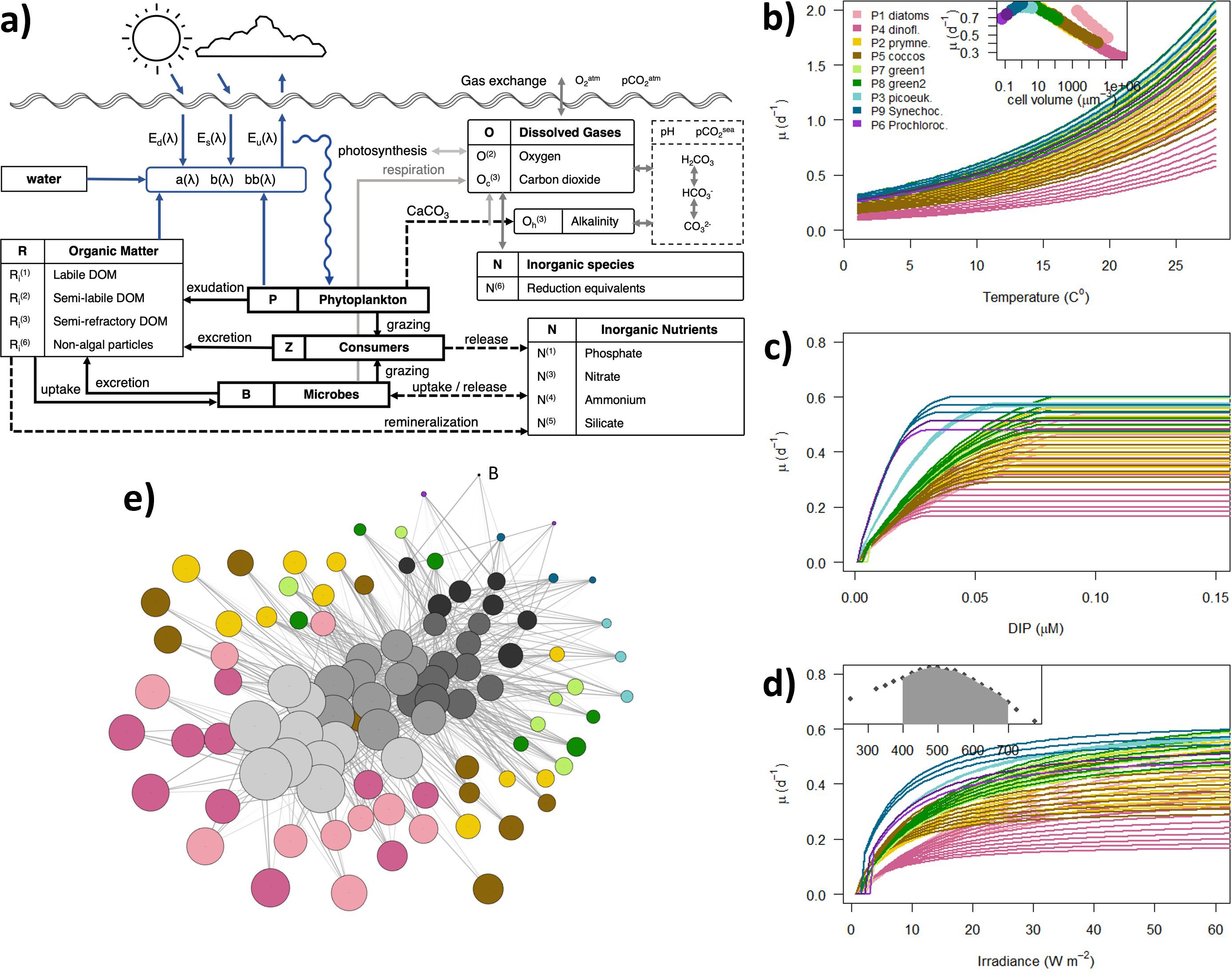
Figure 1. The building of BFM98: (a) General BFM model scheme. Response curves of the growth rate (µ, d^-1) of phytoplankton functional types as a function of model dependencies: (b) temperature, (c) dissolved inorganic phosphorous (DIP) and (d) photosynthetically active radiation (PAR). The curves in panels (b), (c) and (d) were obtained computing the steady state solutions of phytoplankton dynamic (see Phyto.F90 in the Code repository) and considering constant aggregation and grazing; the steady state solutions have been obtained time integrating the model in daily time-steps with an ode solver (library deSolve) until stable stoichiometry was achieved and looping over the shown ranges (x-axis) of model dependencies (temperature and irradiance) and model states (DIP). The insert in panel (b) shows the growth rate as a function of cell volume for a reference temperature of 15°C. The insert in panel (d) shows the spectral composition of incoming irradiance used to compute the steady state solutions. (e) The trophic structure of the biodiversity-capable BFM used in this work. The trophic network has been generated and plotted with the R package igraph 1.5.0 using the Fruchterman-Reingold layout.

2.1 Building the BFM ecosystem with the FABM

The BFM was coded under the conventions of the open-source, Fortran-based Framework for Aquatic Biogeochemical Models (Bruggeman and Bolding, 2014) as described in Álvarez et al. (2023) and now this biogeochemical model, called FABM-BFM hereinafter, is integrated in the distributed version of FABM (Bruggeman et al., 2024). FABM enables complex BGC models to be developed as sets of stand-alone, process-specific modules. These are combined at runtime through coupling links to create a custom-made biogeochemical/ecosystem model. One feature of the modularity of FABM-BFM is that the number of plankton types and their coupling links can be defined at runtime without changing or recompiling the code, by adjusting the fabm.yaml configuration file. The whole structure of the ecosystem used in this work (number of plankton types, size structure, allometric relationships, prey-predator relationships) was defined with the characteristics described in the following sections. The script that generates the fabm.yaml is available in the running repository (see Code Availability Section).

2.1.1 Size structure

In BFM, for phytoplankton (P), we described nine different phytoplankton optical types based on their absorption curves from P⁽¹⁾ to P⁽⁹⁾ (Álvarez et al., 2022). Microbes (B) were only represented by a single type of heterotrofic bacteria (B⁽¹⁾). Phytoplankton and bacteria are grazed by four types of consumers (Z), from Z⁽³⁾ to Z⁽⁶⁾, defined based on their trophic strategy. The existing plankton functional type model (1 B, 9 P and 4 Z) was extended by representing a discrete number of size-classes per functional type, each characterized by a distinct cell volume. We use a geometric scale in octaves (a 2ⁿ series) to discretize the size axis, being size defined as biovolume in µm³. This way, the increasing size-classes turn into equally spaced on a logarithmic scale and the amplitude of the class coincides with the lower limit (Blanco et al., 1994). The whole size rage of the living components goes from n´s of -5 to 31, which represents a total size range from 0.4 µm to 2 mm in equivalent spherical diameter (ESD).

Bacteria was only represented in the smaller size bin, therefore ranging 0.4 to 0.5 µm in ESD. For phytoplankton, P⁽⁶⁾ (Prochlorococcus) has two types ranging from 0.5 to 0.8 µm; P⁽⁹⁾ (Synechococcus) has three types ranging from 0.8 to 1.6 µm; P⁽³⁾ (small-eukaryotes) have three types ranging from 1.24 to 2.5 µm; P⁽⁷⁾ (Chlorophyceae) and P⁽⁸⁾ (Prasinophyceae) have six types each ranging in both cases from 2 to 8 µm; P⁽²⁾ (non-calcifier Prymnesiophyceae) and P⁽⁵⁾ (coccolithophores) have ten types each ranging from 3 to 31.5 µm and from 5 to 63 µm, respectively; P⁽¹⁾ (diatoms) and P⁽⁴⁾ (dinoflagellates) have ten types each ranging in both cases from 15.75 to 159 µm. The four types of zooplankton that BFM defines based on their trophic strategy were extended to represent seven size classes of Z⁽⁶⁾ (heterotrophic nanoflagellates) ranging from 4 to 20 µm in ESD; ten types of Z⁽⁵⁾ (bactivorous/herbivorous microzooplankton) ranging from 10 to 100 µm; ten types of Z⁽⁴⁾ (omnivorous mesozooplankton) ranging from 40 to 400 µm; and ten types of Z⁽³⁾ (carnivorous mesozooplankton) ranging from 200 to 2016 µm.

2.1.2 Phytoplankton (P)

In BFM, the evolution of phytoplankton biomasses is controlled by the net outcome of growth, mortality, aggregation and grazing by zooplankton. Therefore, the formulation of the biological equations is based on mechanistic descriptions of the processes of nutrient uptake, light capture, sinking and predator–prey encounter rates. Phytoplankton growth depends on the nitrogen and phosphate limitations, which are modelled according to a Droop´s quota approach. The production terms for diatoms are defined as for the rest, except that the limitation terms also include silicate. The growth rate of phytoplankton includes a generic temperature dependency (Eppley, 1972).

The size dependence has been included into the formulation of seven phytoplankton traits according to specific literature. The maximum growth rate (P_max) is prescribed to follow a unimodal distribution with cell size (Marañón et al., 2013; Dutkiewicz et al., 2020) (Figure 1b). This way, for a given temperature, intermediate sized individuals have the larger growth rates whereas prokaryotes and small-eukaryotes have intermediate ones and the larger phytoplankton have the smaller ones (see insert in Figure 1b for an example at 15°C). Nitrate and phosphate uptake affinities decrease with cell size (Edwards et al., 2012) as well as the optimum quota of phosphorous (Grover, 1989; minimum and maximum quota were the optimum times 0.55 and 2, respectively). Thus, smaller phytoplankton has advantage at lower nutrients concentrations with respect to larger phytoplankton (Figure 1c). The nine different phytoplankton optical types based on their absorption curves kept all the same photochemical efficiency (4.8·10^–4 mgC µmol quanta^-1) but larger maximum chlorophyll (Chl-a) to carbon ratio (Θ_max) for smaller phytoplankton (Figure 1d). Negative size dependencies have been included into the formulation of the basal respiration rate (Tang, 1995; Irwin et al., 2006) and in the sinking speed (Durante et al., 2019). The volume to carbon conversions were those from Menden-Deuer and Lessard (2000) and differ taxonomically.

2.1.3 Zooplankton (Z)

In BFM, the ingestion rate of the predators varies with the biomass of the predator and the total prey density available to that predator following a Michaelis-Menten function, that depends on the maximum ingestion rate (d^-1), the metabolic temperature response described with a generic temperature dependency (Eppley, 1972) and the relative preference of the predator for each type of prey. The multiple-prey functional response of the predator includes constant preferences fixed in the prey-predator matrix and, optionally, density-dependent preferences.

The size dependence has been included into the formulation of one zooplankton trait and in the grazing preferences according to specific literature. The maximum ingestion rate decreases with organism size following Hansen et al. (1997) and the predetermined prey-predator matrix has been extended by including an explicit size-dependent relationship for the grazing preferences. The grazing preference has a log-normal distribution centered on a predator:prey length ratio of 10 (Kiørboe, 2008) as grazers tend to feed preferentially on preys ten times smaller, with a standard deviation of the logarithm of the preferred length ratio of 0.2 (Banas, 2011). In this work, density dependent preferences have been deactivated (all p_minfood parameters set to 0, see Code repository) and therefore zooplankton types do not modify their attack rate according to the density of individual prey types.

The final trophic network used in this work is shown in Figure 1e where the size of the dots is proportional to the biovolume assigned to the plankton type and color dots represent autotrophic organisms whereas grey-scale dots represent heterotrophic organisms. The width of the coupling links is proportional to the preference in the diet. The graphic tool (library igraph 1.5.0) minimizes the overall length of the predation links, therefore the panel shows how heterotrophic nanoflagellates (darker grey) feed on bacteria (black) and small phytoplankton (blues and greens) whereas larger zooplankton (lighter grey) feeds preferentially on larger phytoplankton (browns and pinks) and zooplankton smaller than themselves (medium grey).

2.1.4 Other BFM compartments

The living components of the ecosystem are completed with a single type of heterotrophic bacteria (B) that feeds on dissolved (DOC) and non-living particulated material (NAP). Bacterial excretion produces semi-refractory dissolved material, contributing to the immobilization of organic carbon, and remineralizes organic compounds to inorganic nutrients (DIN, DIP and Si). Labile and semi-labile DOC is produced as a subproduct of phytoplankton activity and zooplankton-mediated mortality of phytoplankton and bacteria. Detritus (NAP) are produced and a result of zooplankton egestion and slopy feeding. The carbonate system is resolved with DIC and Alkalinity as state variables, and the production of particulated inorganic carbon (PIC) is included as a direct term from DIC to PIC implicitly representing the activity of calcifying phytoplankton (P⁽⁵⁾).

2.2 Testcase 1D

To demonstrate the applicability and how FABM-BFM can be used to develop diversity-capable models, we present the application to the size-structured plankton community model that resolves 60 phytoplankton and 37 zooplankton size classes (BFM98) in a one-dimensional pelagic ocean setting representing an open-ocean ecosystem in the NW Mediterranean Sea, the Bouée pour l’acquisition de Séries Optiques à Long Terme (BOUSSOLE) observatory. The site is visited monthly by oceanographic cruises to collect optical and BGC variables (Golbol et al., 2000). Seawater is generally collected at 12 discrete depths within the 0–400 m water column (5, 10, 20, 30, 40, 50, 60, 70, 80, 150, 200, 400 m). Sampling is performed with a SeaBird SBE911+ CTD/rosette system equipped with pressure (Digiquartz Paroscientific), temperature (SBE3+) and conductivity (SBE4) sensors and 12-L Niskin bottles, from which water samples are collected for subsequent absorption measurements and high-performance liquid chromatography (HPLC) analyses. The HPLC procedure used to measure phytoplankton pigment concentrations is fully described in Ras et al. (2008). The fractions of 3 phytoplankton size classes were calculated following the diagnostic pigments method (DiCicco et al., 2017). Satellite measurements were extracted from the CMEMS daily products of phytoplankton absorption and light extinction coefficient (OCEANCOLOUR_MED_BGC_L3_MY_009_143) averaging a 20x20km box around the BOUSSOLE site (E.U. Copernicus Marine Service Information, 2022).

2.2.1 The 1D vertical setup: GOTM

The General Ocean Turbulence Model (GOTM, Burchard et al., 1999) is a one-dimensional water column build around an extensive library of turbulence closure models that simulates the vertical structure of the water column – notably saline, thermal and turbulence dynamics. The FABM enables the flexible coupling of ecosystem processes into GOTM and therefore allows to perform simulations at 1D locations with GOTM handling hydrodynamics and BFM the biogeochemistry. The vertical setup has the potential to facilitate direct testing of model assumptions in the context of small-scale measurements by observational and laboratory oceanographers. We used the 1D setup for the BOUSSOLE observatory, comprehensively described in Álvarez et al. (2023), where atmospheric forcing is taken from the ECMWF ERA5 dataset, spectral light composition at the top of the ocean from the OASIM model (Lazzari et al., 2021) and T/S and biogeochemical variables from the reanalysis of the Mediterranean Sea biogeochemistry (Cossarini et al., 2021). An initial biomass concentration of 0.1 mg C m^-3 of phytoplankton and 0.08 mg C m^-3 of zooplankton was distributed uniformly over logarithmic size-classes, resulting in concentrations that range from 0.1 to 2·10^–5 mg C m^-3 of each of the 98 possible plankton types (60 phytoplankton, 37 zooplankton and 1 bacteria). To compare BFM98 with a benchmark BFM version, we used the exact same configuration of BFM described in Álvarez et al. (2023) that contains 9 plankton types (4 phytoplankton, 4 zooplankton and 1 bacteria) and called here BFM9. A comparison of computational and storage resources required for running BFM9 and BFM98 is included in the Supplementary Material 1.

2.2.2 Diversity-sustaining mechanism

GOTM-FABM-BFM simulates prognostic 1D distributions of the plankton types concentrations, and the composition of the community emerges from the initial diversity through species sorting (variation of the relative abundance of the species of the system) as a result of the imposed environmental conditions. Most diversity (number of types present) was lost within 10 years if we did not impose diversity-sustaining mechanisms, which indicated that even in a vertically structured setup, the proposed trait variability and the diffusion-mediated dispersal was insufficient for maintenance of a realistic biodiversity. To avoid the loss of diversity (i.e., the restriction of the traits space), as shown by preliminary simulations, we opted for using a species selection approach where all types are present in the system (everything is everywhere) by imposing continuous species immigration and community composition emerges in response to the changing environment (and environment selects). In practice, we imposed the relaxation towards the initial concentrations with a time constant of 5 years to introduce continuously trace quantities of all species that are present at smaller concentrations than their initial values and simultaneously export a fraction of the existing system following Bruggeman and Kooijman (2007). A detailed sensitivity analysis performed to select the minimum immigration rates capable to sustain diversity while keeping the net inflow-outflow of biomass close to zero is included in the Supplementary Material 2.

2.2.3 Final 1D runs: decadal (present) and centennial

The model was integrated forward with a biological time step of 10 min. First, with climatologically averaged atmospheric forcing and T/S profiles for 100 repeated years (CLIM). After approximately 2 years of integration, bulk properties such as total phytoplankton and zooplankton biomass, and diversity indicators, such as number of phytoplankton and zooplankton types present in the community, settled into a repeating seasonal cycle. Secondly, the model was integrated with real-date forcing from 2000 to 2022 (REAL-DATE), and the results compared to observations collected in situ and remotely at the BOUSSOLE site. And third, the model was integrated with climatologically averaged forcing and nutrient concentrations relaxed monthly to decreasing phosphate (N1p) and nitrate (N3n) concentrations from 2000 to 2100 (TREND). The rate of nutrient decrease was set to -13.1% for N1p and -19.8% for N3n, following the trends reported by Reale et al. (2022) for the entire Mediterranean in the first 100m of the water column between present day (2005-2020) and far future (2080-2099) under the 8.5RCP emissions scenario.

3 Analysis

3.1 Model at equilibrium and computing times

Forced with climatologically averaged atmospheric input and initialization, the model settles into a repeated seasonal cycle after approximately 2–3 years of integration. The CLIM simulation does not lose diversity when the biomass of each plankton type is relaxed to their initial concentration with a time constant of 5 years (Supplementary Material 2), which in practice means that all plankton types are always present in the system and the net inflow of biomass to the system is less than 1 ng C L^-1 d^-1. Therefore, from here thereinafter, a plankton type was considered present in the community if the biomass is larger than 0.01 mg C m^-3. Despite the fact that BFM98 contains 386 state variables compared to the 55 of BFM9, the integration and initialization times are less than three times longer (Supplementary Material 1).

3.2 Ecology, biogeochemistry and optics

The annual evolution of real-date bulk biogeochemical properties simulated by BFM9 and BFM98 were compared to observations collected at the DYFAMED and BOUSSOLE observatories. Chl-a concentration (mg Chl-a m^-3) at surface peaks in spring and decreases in summer comparably to in situ measurements (Figure 2a). At the depth of the Chl-a maximum (DCM) the model tends to underestimate Chl-a at the beginning of the summer and overestimate it during summer and autumn. Integrated phytoplankton (Figure 2b) and bacterial biomass (Figure 2c) in the first 130 m of the water column show a clear alternance between phytoplankton and bacterial dominated communities. One remarkable difference between BFM9 and BFM98 is the larger concentrations of phytoplankton in the latter (Figure 2b), concurrent with less bacteria (Figure 2c) and less heterotrophic nanoflagellates (Figure 2d). All zooplankton integrated and mean biomasses tend to peak after spring in relatively good agreement with the scarce observational data (Figures 2e, f), but BFM98 tends to sustain larger biomasses of micro- and meso-zooplankton throughout the year.

Figure 2

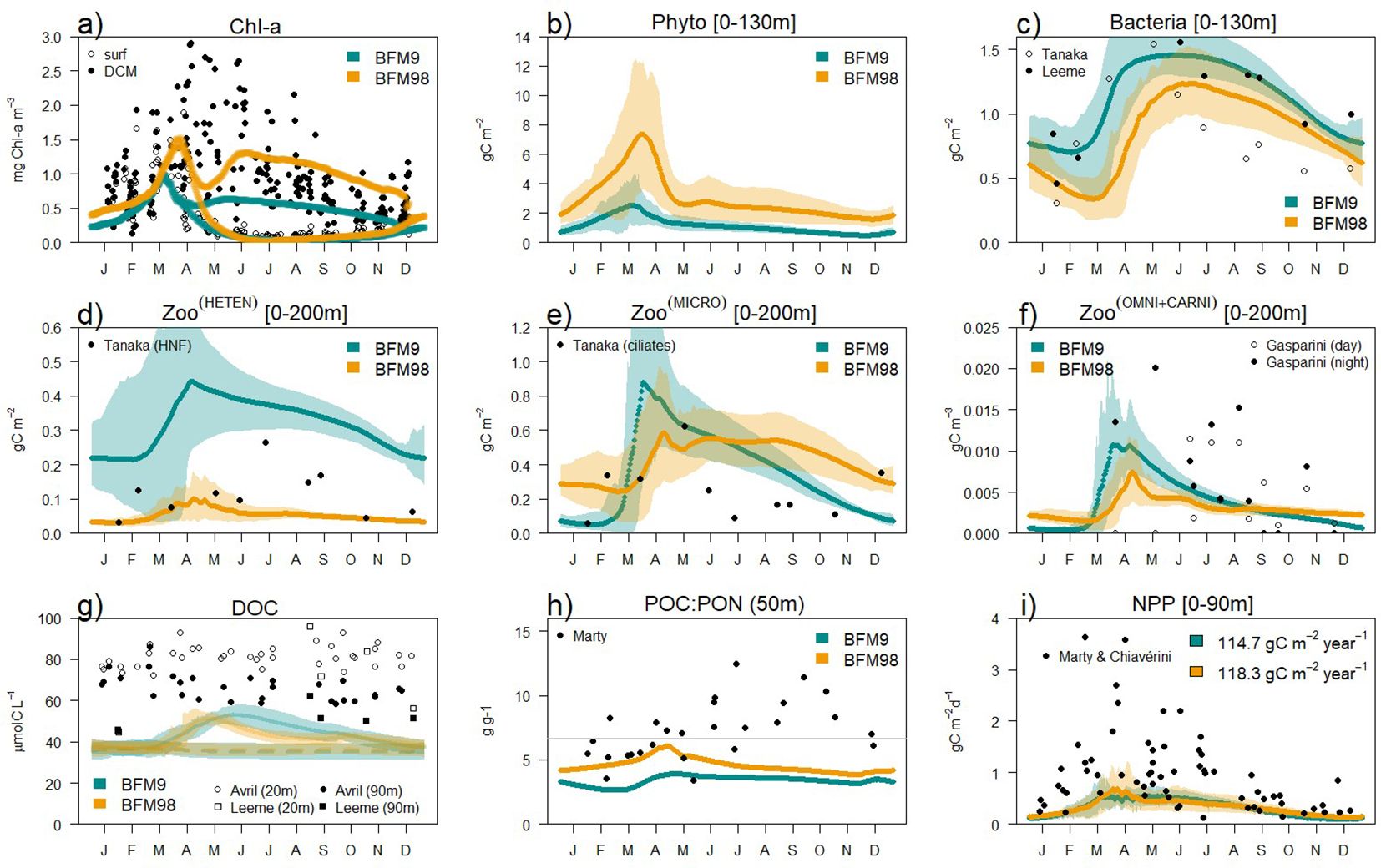
Figure 2. Annual timeseries of biogeochemical indicators simulated by BFM9 (blue solid line) and by BFM98 (orange solid line), with dots showing observations at the BOUSSOLE/DYFAMED sites: (a) Chl-a concentration at surface and at the DCM compared to Antoine and Vellucci (2021); (b) vertically-integrated (0-130m) phytoplankton carbon; (c) vertically-integrated (0-130m) bacterial biomass compared to Lemee et al. (2012) and Tanaka and Marty (2012); (d) vertically-integrated (0-200m) Z⁽⁶⁾ biomass compared to HeteN from Tanaka and Marty (2012); (e) vertically-integrated (0-200m) Z⁽⁵⁾ biomass compared to Ciliates from Tanaka and Marty (2012); (f) mean over 200m of 02 mesozooplankton (Z(3)+Z(4)) biomass, compared to Gasparini et al. (2004); (g) DOC concentration at 20 and 90m compared to Avril (2002) (open dots) and Lemee et al. (2012) (solid dots); (h) POC: PON at 50m compared to Marty (2012); (i) vertically-integrated (0-90m) net primary production, compared to NPP extrapolated from 3-4h incubations and daylength from Marty and Chiavérini (2002).

Dissolved organic carbon concentrations simulated by the model tend to be slightly smaller than those observed but both model configurations are able to capture the accumulation of DOC during summer and autumn in surface (20 m) and the relative lower concentrations at 90m (Figure 2g). The ratio between particulate organic carbon to particulate nitrogen ratio observed at the site tends to be smaller than 6 during spring to become larger in summer, whereas BFM98 (B+P+NAP+Z⁽⁶⁾+Z⁽⁵⁾) tends to be more conservative around the Redfield 6 value and BFM9 be smaller (Figure 2h). Total annual net primary production integrated in the first 90 m simulated is 114.7 and 118.3 gC m^-2 by BFM9 and BFM98, respectively (Figure 2i). In both cases underestimated when compared to short-term incubations done in situ but comparable to estimates in the NW Mediterranean Sea (Siokou-Frangou et al., 2010).

The spectrally-resolved version of BFM resolves light transmission in the water column as it is absorbed and scattered by water, phytoplankton, CDOM and detritus. Figure 3a shows the vertical distribution (0 to 200 m) of total Chl-a concentration along an average year. The simulated Chl-a accumulates in spring in the first 30 m to later remain confined to deeper layers from 40 m at the beginning of the summer to around 55 m in autumn (Figure 3a), in a pattern observed at the site (Antoine et al., 2006) and in general in the open waters of the NW Mediterranean Sea (Lavigne et al., 2015). The inherent optical properties simulated in the proposed configuration were consistent with previous lower complexity versions of the model (Álvarez et al., 2023) with a_PH(450) following the distribution of Chl-a (Figure 3b) and a_CDOM(450) forming a sub-superficial maximum in summer (Figure 3c). The contribution of NAP to total non-water absorption [a_NAP(450)] is slightly larger during spring given a large presence of detritus (not shown). The annual evolution of simulated a_PH(450) (Figure 3d) and light extinction coefficient (k_D(490), Figure 3e) was compared to observations collected remotely in the north west Mediterranean Sea, showing a relative good agreement. BFM98 tends to simulate slightly lower k_D(490) out of the spring bloom compared to BFM9.

Figure 3

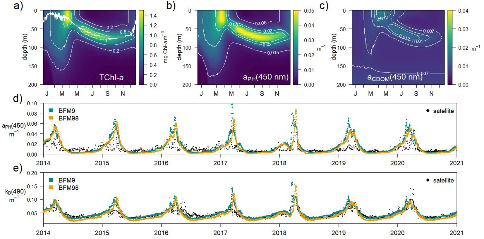
Figure 3. Annually-averaged (a) vertical profile of total Chl-a concentration at the BOUSSOLE site and IOPs: (b) a_PH(450nm) and (c) a_CDOM(450nm), in the BFM98 present simulation. Timeseries of (d) a_PH(450nm) and (e) k_D(490nm) fitted to E₀(490nm) in the first optical depth (z_EU/4.6), in the BFM9 and BFM98 present simulations, compared to the timeseries of CMEMS products at the site (black dots).

3.3 Phytoplankton community composition and diversity indicators

The simulated vertical distribution (0 to 200 m) and temporal variation (January to December) of phytoplankton size classes according to Chl-a concentrations (Figure 4 right panels) is consistent in shape and magnitude with observations derived from HPLC data (Figure 4 left panels), which clearly reveal the dominance of nanoplankton in the site and the importance of diatoms and picoplankton in the bloom and in the summer DCM, respectively (see Álvarez et al. (2023) for the same analysis of PSCs at BOUSSOLE with BFM9). A visual comparison of the dominance of different phytoplankton size classes at the DCM throughout the year (Figure 4 bottom panels) shows how the diatoms in the model seem to peak later than observed and nanoflagellates tend to dominate the early bloom whereas picoplankton dominates later in the year.

Figure 4

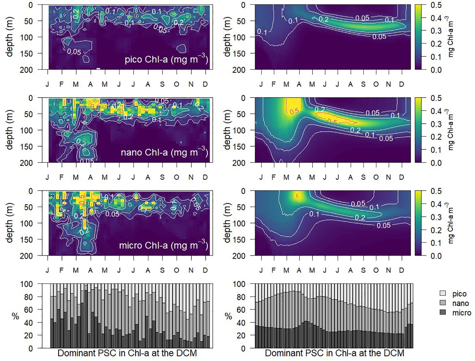
Figure 4. Annually-averaged vertical profiles of Chl-a size-classes (PSC) (pico, nano and micro, from top to bottom) in BOUSSOLE observations (left) and in model simulations (right). Bottom panel shows the relative contribution of PSCs Chl-a to total Chl-a at the depth of the Chl-a maximum (DCM) each week. The asymmetry at the end/start of the year in the BOUSSOLE data is caused by the absence of observational data consistently throughout the timeseries from 17^th Dec to 18^th Jan.

The number of phytoplankton and zooplankton types present in the community (functional richness) across different years indicates seasonal variations and inter-annual trends. On the y-axis, Figure 5 shows the functional richness of both the phytoplankton and zooplankton community. Each line represents the simulation of a different year from 2000 to 2022, color-coded accordingly. For phytoplankton, while most changes in richness at surface are driven by the abrupt increase in biomass of the spring bloom (Figure 5a), when the DCM is formed richness remains low (Figure 5b) despite relatively high values of biomass (Figure 2a). Richness of zooplankton types is less variable; at any given point in time only 14 to 20 types are present in the community both at surface (Figure 5c) and at the DCM (Figure 5d).

Figure 5

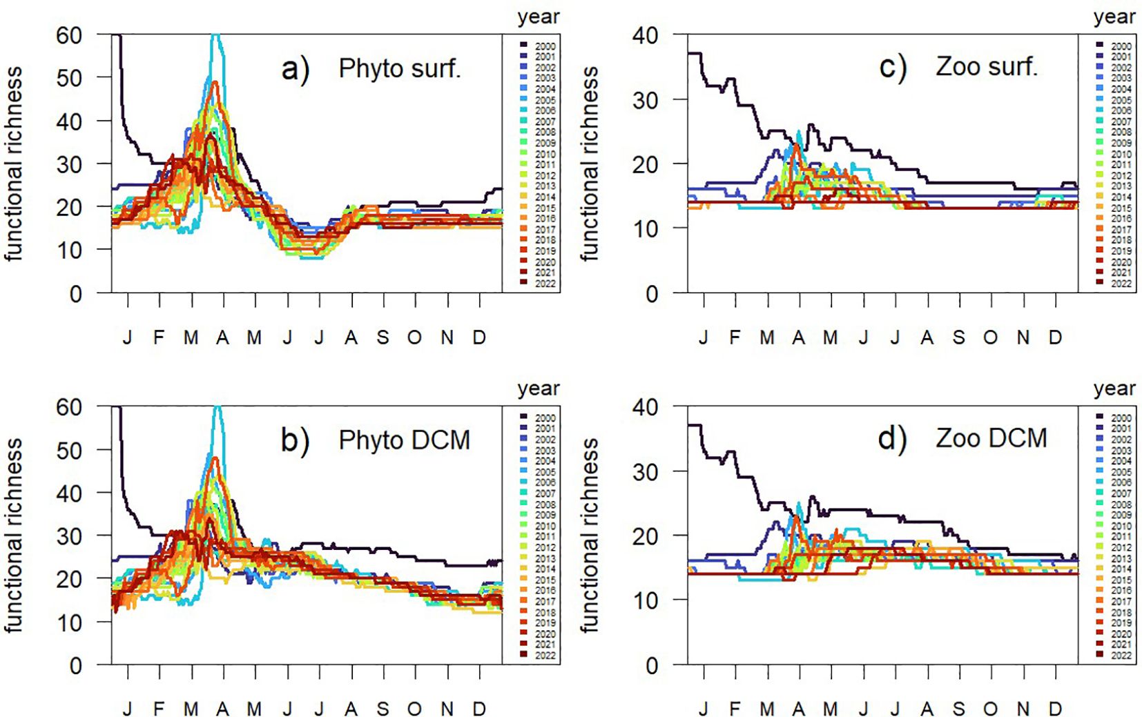
Figure 5. Annual timeseries of the number of phytoplankton and zooplankton types present in the community (functional richness) along the 22 years simulated by BFM98: phytoplankton functional richness (a) at surface and (b) at the depth of the Chl-a maximum (DCM), and zooplankton functional richness (c) at surface and (d) at the DCM.

3.4 Eco-evolutionary history of the simulated plankton community

The CLIM simulations, where BFM98 was integrated forward with climatologically averaged atmospheric forcing during 100 repeated years, showed that after the first 2–3 years, no significant drift in the functional richness of phytoplankton (Figure 6a) nor zooplankton (not shown) was observed. The TREND simulation was identical to CLIM, except that it included a constant decrease in nutrient concentrations from 2005 to 2099 of -13.1% in phosphate and -19.8% in nitrate. Phytoplankton richness in TREND (Figure 6b) showed smaller seasonal amplitude by the end of the hundred years. To explore such differences between CLIM and TREND, we employed community turnover. Community turnover computes the difference in plankton types in two timepoints as the total number of types gained (NG) and/or lost (NL) with respect to the total number of types observed in both timepoints (NT). The month-to-month turnover (Righetti et al., 2019) computes the average turnover ((NG+NL)/NT) between all consecutive months of the year, therefore mainly capturing the seasonal differences in community composition. The seasonal turnover of the climatological run (CLIM) stabilizes after approximately one decade around 0.17 (Figure 6c), but it shows some variability around this value. The seasonal turnover of the TREND run is smaller and reaches 0.10 at the end of the 100 years, corroborating the smaller seasonal differences in phytoplankton community composition with decreasing nutrient availability, and, in practice, indicating that the model diversity is able to change in response to environmental forcing.

Figure 6

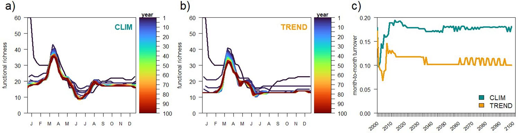
Figure 6. Diversity indicators (richness & turnover) in centennial simulations. Number of phytoplankton types present in the community (functional richness) (a) along hundred repetitions of the same climatological year (CLIM) and (b) along hundred years with decreasing nitrate and phosphate availability (TREND). (c) Annually averaged phytoplankton community month-to-month turnover in the CLIM and TREND simulations.

4 Discussion

We present a coupled optical-biogeochemical ecosystem model designed for exploring the emergent patterns of plankton distributions and understanding current and future changes in marine plankton diversity, while keeping the bulk biogeochemistry and optical behavior consistent with observations. We present a case study at the BOUSSOLE site as our proof of concept, where biogeochemical and optical indicators as well as the general behavior of the modeled ecosystem seem to be in agreement with the observed dynamics at the site. Although further analyses using observed data in other locations are necessary to establish the validity of the results obtained, the tools and configuration presented here will be instrumental for future applications of the Biogeochemical Flux Model (BFM) in 3D domains and under climatic projections.

The development of biodiversity-capable plankton models is rapidly advancing, contributing to a growing but still limited body of literature on biogeochemical models that allow simulating ecosystem diversity (Follows et al., 2007), focused on advancing our understanding of ecological interactions, community dynamics, and evolutionary processes. Our model represents the first diversity-capable mechanistic model implemented in the Mediterranean Sea, aligns with current state-of-the-art ecological models capable of representing a couple of hundreds of discrete plankton types (e.g. Dutkiewicz et al., 2020) while simultaneously being lightweight enough to be integrated at centuries scale.

4.1 Ecological implications

The ability to simulate realistic plankton diversity beyond the current state-of-the-art models that rely on functional types and aggregated taxa, alongside biogeochemistry can reveal previously unrecognized dynamics in plankton community interactions and their cascading effects on biogeochemical cycles. By explicitly representing a diverse plankton community, our model facilitates future research into the interplay between biogeochemical fluxes and biodiversity. Changes in plankton diversity may have profound implications for ecosystem functioning, as they can influence primary production and nutrient remineralization pathways given differential nutrient uptake strategies among coexisting phytoplankton groups (Kwon et al., 2022); alter the efficiency of the biological carbon pump, since size and other particle properties influence particle sinking and fluxes (Cael et al., 2021a); and influence and the energy transfer across trophic levels though shifts in predator-prey interactions and trophic dynamics (Serra-Pompei et al., 2022).

4.2 Evolutionary implications

Our diversity-capable FABM-BFM model incorporates species selection through migration, and thanks to the species selection approach implemented formally through migration (Bruggeman and Kooijman, 2007), effectively representing eco-evolutionary processes that influence community dynamics. By defining a sufficiently complex and broad trait space, the model allows for adaptive shifts in community structure in response to environmental conditions, implicitly capturing how marine communities alter their functional structure, relocate, or adapt in response to environmental shifts. Investigating diversity-sustaining mechanisms is an active area of research and a diversity-capable model as this presented could be used as a laboratory to test those, including the role of trophic interactions (Edwards and Yool, 2000; Vallina et al., 2014), transport (Junger et al., 2023) or even explicit adaptation (Sauterey et al., 2015; Le Gland et al., 2021) could be further explored. The explicit representation of evolutionary dynamics is beyond the scope of this work, but could complement this approach in future studies, given that the role that evolution plays in marine microbial ecology and carbon cycling is intriguing (Ward et al., 2019). Whether it is implicit or explicitly, to incorporate the processes of adaptation into biogeochemical models is a pressing need as there is increasing observational evidence for significant regional regime shifts at the microbial level particularly in response to climate change (e.g Cael et al., 2021b). Exploring the evolutionary aspects of plankton diversity could offer important insights into how these communities may adapt to changing environmental conditions in the coming decades.

4.3 Challenges of representing many discrete plankton types

One of the fundamental challenges that diverse-capable ecosystem models face is the trade-off between increasing complexity and the resulting increase in uncertainty. As models incorporate more plankton types to capture the intricate dynamics of marine ecosystems, they can improve the representation of diverse species interactions, biogeochemical cycles, and ecosystem functions. However, it also introduces greater uncertainty, as more parameters need to be estimated and many interactions remain poorly understood or data-limited. Balancing this trade-off requires careful calibration and validation. A diversity capable module developed within a coupled optical-biogeochemical model permits the whole system to be constrained by multiple observational datasets, including those biogeochemical and optical, and furthermore incorporating novel sources of observational data, such as high-throughput plankton imaging (Pierella Karlusich et al., 2022) or molecular data (Levine et al., 2025).

One key challenge in modeling biodiversity through discrete plankton types is scalability. Like other trait-based models (Dutkiewicz et al., 2020), our model captures only a fraction of biodiversity, highlighting a fundamental limitation of our approach: the trait variability included in the model dictates its ability to simulate biodiversity responses to environmental changes. In the BFM98 configuration, the phytoplankton community composition is dynamic, but future model development should incorporate additional traits (such as temperature optima) to better represent ecosystem shifts under multifaceted environmental change. Such further refinement in resolving species-level interactions and fine-scale ecological processes could enhance the predictive power and accuracy of the proposed model in simulating future changes under varying climatic conditions.

4.4 Advantages of the integrated framework

Under the light of those challenges, the modular and scalable nature of FABM-BFM presents several advantages. Traditional models with discrete plankton types become computationally expensive as the number of state variables increases. However, the flexibility of FABM-BFM allows for dynamic ecosystem configurations at runtime, enabling more efficient computational scaling. The 1D versions of the FABM-BFM are relatively fast, making it feasible to conduct extensive analyses that require numerous simulations, such as sensitivity testing of model assumptions or data assimilation procedures. This also makes century-long experiments highly achievable and facilitates the transition to three-dimensional configurations. Additionally, the possibility to perform multi-model simulations is especially valuable for exploring biodiversity-related questions (Jones and Cheung, 2015). Such multi-model ensemble approach (facilitated by FABM) is an essential aspect to perform scenario simulations and associate uncertainties in model projections, that become more robust with respect to the potential differences among the specific ecological models.

By allowing the representation of multiple traits in a broad trait space, FABM-BFM can simulate biodiversity under climatic projections, and explore how predicted changes in diversity could impact ocean biogeochemistry, ocean-color and ecosystem stability or resilience. A key advantage of the proposed framework in this regard is that it is built on the BFM, which underpins the operational biogeochemical products provided by the Copernicus Marine Service (Coppini et al., 2023). Incorporating biodiversity into the BFM framework enhances its potential for future operational applications, particularly in the context of climate change.

4.5 Limitations and future lines of work

Despite the advancements presented in this study, several limitations remain that future work should address. First, the model does not yet incorporate all relevant ecological traits, such as thermal norms (see Supplementary Material 1) that determine species’ temperature-dependent performance. Including these traits would improve the ability of the model to simulate species distributions and community responses to climate variability. Second, while our approach allows for the representation of several hundred plankton types, it remains a simplified functional-type framework. Furthermore, the model has not yet been systematically compared to more detailed species-level models or real-world plankton community observations. Assessing how well the current biodiversity representation captures observed ecological processes and community dynamics is a necessary step for further validation and refinement. Finally, the absence of lateral transport in the 1D configuration constrains the influence of connectivity, necessitating prescribed migration fluxes to approximate transport effects. A key question for future work is whether the transport processes in a fully three-dimensional implementation would be sufficient to maintain diversity, or if additional ecological processes must be incorporated to sustain realistic plankton community structures over time, such as more complex predator-prey dynamics or automatic differentiation of traits.

5 Conclusions

Our results provide a baseline configuration for future applications of the 1D BFM under realistic external forcing. The diversity-capable BFM presents multiple potential applications, including simulating plankton diversity changes under climate projections, assessing feedbacks between phytoplankton community structure and biogeochemical cycles, and exploring links between biodiversity and ocean color remote sensing. Future work should focus on expanding trait diversity, integrating additional adaptive mechanisms, and transitioning to three-dimensional model configurations to further enhance predictive capabilities in a changing ocean.

Data availability statement

The datasets presented in this study can be found in online repositories. The names of the repository/repositories and accession number(s) can be found below: GOTM: https://www.github.com/gotm-model; FABM: https://github.com/fabm-model/fabm.git; Setup BOUSSOLE: https://github.com/ealvarez-s/setup_BFM1D_BOUSSOLE.git; BOUSSOLE project: http://www.obs-vlfr.fr/Boussole/html/boussole_data/other_useful_files.php; DYFAMED datasets: https://doi.org/10.1594/PANGAEA.803600; https://doi.org/10.1594/PANGAEA.183618; https://doi.org/10.1594/PANGAEA.803612; https://doi.org/10.1594/PANGAEA.803605; https://doi.org/10.1594/PANGAEA.738606; https://doi.org/10.1594/PANGAEA.803611.

Author contributions

EÁ: Conceptualization, Data curation, Formal Analysis, Methodology, Software, Visualization, Writing – original draft, Writing – review & editing, Validation. GO: Data curation, Software, Writing – review & editing. GC: Conceptualization, Funding acquisition, Project administration, Supervision, Writing – review & editing. CS: Conceptualization, Funding acquisition, Project administration, Writing – review & editing. PL: Conceptualization, Funding acquisition, Software, Supervision, Writing – review & editing.

Funding

The author(s) declare that financial support was received for the research and/or publication of this article. This work has received funding from the European Union’s Horizon Europe research and innovation action under grant agreement No 101081273 (project NECCTON) and from the National Biodiversity Future Center (NBFC) funded by the Piano Nazionale di Ripresa e Resilienza (NextGenerationEU). The GOTM-FABM-BFM model has been implemented in the framework of the SEAMLESS project, funded by the European Union’s Horizon 2020 research and innovation program under grant agreement No 101004032. The CINECA HPC consortium provided high-performance computing resources and support.

Acknowledgments

The Laboratoire d’Océanographie de Villefranche provided publicly datasets at the BOUSSOLE and DYFAMED stations. The authors want to acknowledge Jorn Bruggeman (B&B) and Stefano Campanella (OGS) for guiding us on the code profiling and Sergio Vallina (IEO-CSIC) and Pedro Cermeño (ICM-CSIC) for insightful discussions on an early stage of the manuscript.

Conflict of interest

The authors declare that the research was conducted in the absence of any commercial or financial relationships that could be construed as a potential conflict of interest.

Generative AI statement

The author(s) declare that no Generative AI was used in the creation of this manuscript.

Publisher’s note

All claims expressed in this article are solely those of the authors and do not necessarily represent those of their affiliated organizations, or those of the publisher, the editors and the reviewers. Any product that may be evaluated in this article, or claim that may be made by its manufacturer, is not guaranteed or endorsed by the publisher.

Supplementary material

The Supplementary Material for this article can be found online at: https://www.frontiersin.org/articles/10.3389/fevo.2025.1504518/full#supplementary-material

References

Acevedo-Trejos E., Brandt G., Bruggeman J., and Merico A. (2015). Mechanisms shaping size structure and functional diversity of phytoplankton communities in the ocean. Sci. Rep. 5, 8918. doi: 10.1038/srep08918

PubMed Abstract | Crossref Full Text | Google Scholar

Álvarez E., Cossarini G., Teruzzi A., Bruggeman J., Bolding K., Ciavatta S., et al. (2023). Chromophoric dissolved organic matter dynamics revealed through the optimization of a spectrally and vertically resolved model in the NW Mediterranean Sea. Biogeosciences 20, 4591–4624. doi: 10.5194/bg-20-4591-2023

Crossref Full Text | Google Scholar

Álvarez E., Lazzari P., and Cossarini G. (2022). Phytoplankton diversity emerging from chromatic adaptation and competition for light. Prog. Oceanogr. 204, 102789. doi: 10.1016/j.pocean.2022.102789

Crossref Full Text | Google Scholar

Antoine D., Chami M., Claustre H., D’Ortenzio F., Morel A., Bécu G., et al. (2006). BOUSSOLE: A joint CNRS-INSU, ESA, CNES and NASA ocean color calibration and validation activity, NASA technical memorandum no. 2006 – 214147. Available online at: https://ntrs.nasa.gov/citations/20070028812 (Accessed May 5, 2025).

Google Scholar

Antoine D. and Vellucci V. (2021).BOUSSOLE project: HPLC dataset. In: BOUSSOLE project. Available online at: http://www.obs-vlfr.fr/Boussole/html/boussole_data/other_useful_files.php (Accessed November 29, 2022).

Google Scholar

Avril B. (2002). Dissolved organic carbon measured on water bottle samples at time series station DYFAMED. PANGAEA. doi: 10.1594/PANGAEA.803600

Crossref Full Text | Google Scholar

Banas N. S. (2011). Adding complex trophic interactions to a size-spectral plankton model: Emergent diversity patterns and limits on predictability. Ecol. Modell 222, 2663–2675. doi: 10.1016/j.ecolmodel.2011.05.018

Crossref Full Text | Google Scholar

Blanco J. M., Echevarría F., and García C. M. (1994). Dealing with size-spectra: some conceptual and mathematical problems. Sci. Mar. 58 (1-2), 17–29.

Google Scholar

Bruggeman J. and Bolding K. (2014). A general framework for aquatic biogeochemical models. Environ. Modell Softw. 61, 249–265. doi: 10.1016/j.envsoft.2014.04.002

Crossref Full Text | Google Scholar

Bruggeman J., Bolding K., Nerger L., Teruzzi A., Spada S., Skákala J., et al. (2024). EAT v1.0.0: a 1D test bed for physical–biogeochemical data assimilation in natural waters. Geosci. Model Dev. 17, 5619–5639. doi: 10.5194/gmd-17-5619-2024

Crossref Full Text | Google Scholar

Bruggeman J. and Kooijman S. A. L. M. (2007). A biodiversity-inspired approach to aquatic ecosystem modeling. Limnol. Oceanogr. 52, 1533–1544. doi: 10.4319/lo.2007.52.4.1533

Crossref Full Text | Google Scholar

Burchard H., Bolding K., and Villarreal M. (1999). GOTM, a general ocean turbulence model: Theory, implementation and test cases. Report EUR 18745. Available online at: https://op.europa.eu/publication-detail/-/publication/5b512e12-367d-11ea-ba6e-01aa75ed71a1 (Accessed May 5, 2025).

Google Scholar

Cael B. B., Cavan E. L., and Britten G. L. (2021a). Reconciling the size-dependence of marine particle sinking speed. Geophys. Res. Lett. 48, e2020GL09177. doi: 10.1029/2020GL091771

Crossref Full Text | Google Scholar

Cael B. B., Dutkiewicz S., and Henson S. (2021b). Abrupt shifts in 21st-century plankton communities. Sci. Adv. 7, eabf8593. doi: 10.1126/sciadv.abf8593

PubMed Abstract | Crossref Full Text | Google Scholar

Coppini G., Clementi E., Cossarini G., Salon S., Korres G., Ravdas M., et al. (2023). The mediterranean forecasting system – part 1: evolution and performance. Ocean Sci. 19, 1483–1516. doi: 10.5194/os-19-1483-2023

Crossref Full Text | Google Scholar

Cossarini G., Feudale L., Teruzzi A., Bolzon G., Coidessa G., Solidoro C., et al. (2021). High-resolution reanalysis of the mediterranean sea biogeochemistry, (1999–2019). Front. Mar. Sci. 8. doi: 10.3389/fmars.2021.741486

Crossref Full Text | Google Scholar

DiCicco A., Sammartino M., Marullo S., and Santoleri R. (2017). Regional empirical algorithms for an improved identification of phytoplankton functional types and size classes in the Mediterranean sea using satellite data. Front. Mar. Sci. 4. doi: 10.3389/fmars.2017.00126

Crossref Full Text | Google Scholar

Durante G., Basset A., Stanca E., and Roselli L. (2019). Allometric scaling and morphological variation in sinking rate of phytoplankton. J. Phycol. 55, 1386–1393. doi: 10.1111/jpy.12916

PubMed Abstract | Crossref Full Text | Google Scholar

Dutkiewicz S., Cermeño P., Jahn O., Follows M. J., Hickman A. A., Taniguchi D. A. A., et al. (2020). Dimensions of marine phytoplankton diversity. Biogeosciences 17, 609–634. doi: 10.5194/bg-17-609-2020

Crossref Full Text | Google Scholar

Edwards K. F., Thomas M. K., Klausmeier C. A., and Litchman E. (2012). Allometric scaling and taxonomic variation in nutrient utilization traits and maximum growth rate of phytoplankton. Limnol. Oceanogr. 57, 554–566. doi: 10.4319/lo.2012.57.2.0554

Crossref Full Text | Google Scholar

Edwards A. M. and Yool A. (2000). The role of higher predation in plankton population models. J. Plankton Res. 22, 1085–1112. doi: 10.1093/plankt/22.6.1085

Crossref Full Text | Google Scholar

Eppley R. W. (1972). Temperature and phytoplankton growth in the sea. Fish. Bull. 70, 1063–1085.

Google Scholar

E.U. Copernicus Marine Service Information (2022). Mediterranean Sea Ocean Colour Plankton, Reflectance, Transparency and Optics MY L3 daily observations. doi: 10.48670/moi-00299

Crossref Full Text | Google Scholar

Follows M. J., Dutkiewicz S., Grant S., and Chisholm S. W. (2007). Emergent biogeography of microbial. Sci. (1979) 315, 1843–1846. doi: 10.1126/science.1138544

PubMed Abstract | Crossref Full Text | Google Scholar

Gasparini S., Mousseau L., and Marty J.-C. (2004). Zooplankton biomass at DYFAMED time series station. PANGAEA. doi: 10.1594/PANGAEA.183618

Crossref Full Text | Google Scholar

Golbol M., Vellucci V., and Antoine D. (2000). BOUSSOLE. doi: 10.18142/1.

Crossref Full Text | Google Scholar

Grover J. P. (1989). Influence of cell shape and size on algal competitive ability. J. Phycol. 25, 402–405. doi: 10.1111/j.1529-8817.1989.tb00138.x

Crossref Full Text | Google Scholar

Hansen P. J., Bjørnsen P. K., and Hansen B. W. (1997). Zooplankton grazing and growth: Scaling within the 2-2000 μm body size range. Limnol. Oceanogr. 42, 687–704. doi: 10.4319/lo.1997.42.4.0687

Crossref Full Text | Google Scholar

Hood R. R., Laws E. A., Armstrong R. A., Bates N. R., Brown C. W., Carlson C. A., et al. (2006). Pelagic functional group modeling: Progress, challenges and prospects. Deep Sea Res. Part II: Top. Stud. Oceanogr. 53, 459–512. doi: 10.1016/j.dsr2.2006.01.025

Crossref Full Text | Google Scholar

Irwin A. J., Finkel Z. V., Schofield O. M. E., and Falkowski P. G. (2006). Scaling-up from nutrient physiology to the size-structure of phytoplankton communities. J. Plankton Res. 28, 459–471. doi: 10.1093/plankt/fbi148

Crossref Full Text | Google Scholar

Ismail K. A. and Al-Shehhi M. R. (2023). Applications of biogeochemical models in different marine environments: a review. Front. Environ. Sci. 11. doi: 10.3389/fenvs.2023.1198856

Crossref Full Text | Google Scholar

Jones M. C. and Cheung W. W. L. (2015). Multi-model ensemble projections of climate change effects on global marine biodiversity. ICES J. Marine Sci. 72, 741–752. doi: 10.1093/icesjms/fsu172

Crossref Full Text | Google Scholar

Junger P. C., Sarmento H., Giner C. R., Mestre M., Sebastián M., Morán X. A. G., et al. (2023). Global biogeography of the smallest plankton across ocean depths. Sci. Adv. 9, eadg9763. doi: 10.1126/sciadv.adg9763

PubMed Abstract | Crossref Full Text | Google Scholar

Kiørboe T. (2008). A mechanistic approach to plankton ecology (Princeton, New Jersey: Princeton Univ. Press). 209 pp.

Google Scholar

Kwon E. Y., Sreeush M. G., Timmermann A., Karl D. M., Church M. J., Lee S.-S., et al. (2022). Nutrient uptake plasticity in phytoplankton sustains future ocean net primary production. Sci. Adv. 8, eadd2475. doi: 10.1126/sciadv.add2475

PubMed Abstract | Crossref Full Text | Google Scholar

Lavigne H., D’Ortenzio F., Ribera D’Alcalà M., Claustre H., Sauzède R., and Gacic M. (2015). On the vertical distribution of the chlorophyll a concentration in the Mediterranean Sea: a basin-scale and seasonal approach. Biogeosciences 12, 5021–5039. doi: 10.5194/bg-12-5021-2015

Crossref Full Text | Google Scholar

Lazzari P., Salon S., Terzić E., Gregg W. W., D’Ortenzio F., Vellucci V., et al. (2021). Assessment of the spectral downward irradiance at the surface of the Mediterranean Sea using the radiative Ocean-Atmosphere Spectral Irradiance Model (OASIM). Ocean Sci. 17, 675–697. doi: 10.5194/os-17-675-2021

Crossref Full Text | Google Scholar

Lazzari P., Solidoro C., Ibello V., Salon S., Teruzzi A., Béranger K., et al. (2012). Seasonal and inter-annual variability of plankton chlorophyll and primary production in the Mediterranean Sea: A modelling approach. Biogeosciences 9, 217–233. doi: 10.5194/bg-9-217-2012

Crossref Full Text | Google Scholar

Le Gland G., Vallina S. M., Smith S. L., and Cermeño P. (2021). SPEAD 1.0 – Simulating Plankton Evolution with Adaptive Dynamics in a two-trait continuous fitness landscape applied to the Sargasso Sea. Geosci. Model Dev. 14, 1949–1985. doi: 10.5194/gmd-14-1949-2021

Crossref Full Text | Google Scholar

Lemee R., Gattuso J.-P., and Marty J.-C. (2012). Bacterial production and respiration measured on water bottle samples at time series station DYFAMED. PANGAEA. doi: 10.1594/PANGAEA.803612

Crossref Full Text | Google Scholar

Levine N. M., Alexander H., Bertrand E. M., Coles V. J., Dutkiewicz S., Leles S. G., et al. (2025). Microbial ecology to ocean carbon cycling: from genomes to numerical models. Annu. Rev. Earth Planet Sci. 53 (23), 1–23.30. doi: 10.1146/annurev-earth-040523-020630

Crossref Full Text | Google Scholar

Marañón E., Cermeño P., Lopez-Sandoval D. C., Rodriguez-Ramos T., Sobrino C., Huete-Ortega M., et al. (2013). Unimodal size scaling of phytoplankton growth and the size dependence of nutrient uptake and use. Ecol. Lett. 16, 371–379. doi: 10.1111/ele.12052

PubMed Abstract | Crossref Full Text | Google Scholar

Marty J.-C. (2012). Particulate organic carbon and nitrogen measured on water bottle samples at time series station DYFAMED. PANGAEA. doi: 10.1594/PANGAEA.803605

Crossref Full Text | Google Scholar

Marty J.-C. and Chiavérini J. (2002). Primary production at time series station DYFAMED. PANGAEA. doi: 10.1594/PANGAEA.738606

Crossref Full Text | Google Scholar

Menden-Deuer S. and Lessard E. J. (2000). Carbon to volume relationships for dinoflagellates, diatoms and other protist plankton. Limnol. Oceanogr. 45, 569–579. doi: 10.4319/lo.2000.45.3.0569

Crossref Full Text | Google Scholar

Pierella Karlusich J. J., Lombard F., Irisson J.-O., Bowler C., and Foster R. A. (2022). Coupling imaging and omics in plankton surveys: state-of-the-art, challenges, and future directions. Front. Mar. Sci. 9. doi: 10.3389/fmars.2022.878803

Crossref Full Text | Google Scholar

Ras J., Claustre H., and Uitz J. (2008). Spatial variability of phytoplankton pigment distributions in the Subtropical South Pacific Ocean: comparison between in situ and predicted data. Biogeosciences 5, 353–369. doi: 10.5194/bg-5-353-2008

Crossref Full Text | Google Scholar

Reale M., Cossarini G., Lazzari P., Lovato T., Bolzon G., Masina S., et al. (2022). Acidification, deoxygenation, and nutrient and biomass declines in a warming Mediterranean Sea. Biogeosciences 19, 4035–4065. doi: 10.5194/bg-19-4035-2022

Crossref Full Text | Google Scholar

Righetti D., Vogt M., Gruber N., Psomas A., and Zimmermann N. E. (2019). Global pattern of phytoplankton diversity driven by temperature and environmental variability. Sci. Adv. 5, eaau6253. doi: 10.1126/sciadv.aau6253

PubMed Abstract | Crossref Full Text | Google Scholar

Sauterey B., Ward B. A., Follows M. J., Bowler C., and Claessen D. (2015). When everything is not everywhere but species evolve: an alternative method to model adaptive properties of marine ecosystems. J. Plankton Res. 37, 28–47. doi: 10.1093/plankt/fbu078

PubMed Abstract | Crossref Full Text | Google Scholar

Serra-Pompei C., Hickman A., Britten G. L., and Dutkiewicz S. (2023). Assessing the potential of backscattering as a proxy for phytoplankton carbon biomass. Global Biogeochem. Cycles 37, e2022GB007556. doi: 10.1029/2022GB007556

Crossref Full Text | Google Scholar

Serra-Pompei C., Ward B. A., Pinti J., Visser A. W., Kiørboe T., and Andersen K. H. (2022). Linking plankton size spectra and community composition to carbon export and its efficiency. Global Biogeochem. Cycles 36, e2021GB007275. doi: 10.1029/2021GB007275

Crossref Full Text | Google Scholar

Siokou-Frangou I., Christaki U., Mazzocchi M. G., Montresor M., Ribera d’Alcalá M., Vaqué D., et al. (2010). Plankton in the open Mediterranean Sea: a review. Biogeosciences 7, 1543–1586. doi: 10.5194/bg-7-1543-2010

Crossref Full Text | Google Scholar

Tanaka T. and Marty J.-C. (2012). Microbial carbon biomass and abundance measured on water bottle samples at time series station DYFAMED. PANGAEA. doi: 10.1594/PANGAEA.803611

Crossref Full Text | Google Scholar

Tang E. P. Y. (1995). The allometry of algal growth and respiration. (PhD Thesis), McGill University, Montreal. Available online at: https://escholarship.mcgill.ca/concern/theses/7p88cj69p (Accessed May 5, 2025).

Google Scholar

Terzić E., Miró A., Organelli E., Kowalczuk P., D’Ortenzio F., and Lazzari P. (2021). Radiative transfer modeling with Biogeochemical-Argo float data in the Mediterranean Sea. J. Geophys. Res-Oceans 126, e2021JC01769. doi: 10.1029/2021JC017690

PubMed Abstract | Crossref Full Text | Google Scholar

Vallina S. M., Cermeño P., Dutkiewicz S., Loreau M., and Montoya J. M. (2017). Phytoplankton functional diversity increases ecosystem productivity and stability. Ecol. Modell 361, 184–196. doi: 10.1016/j.ecolmodel.2017.06.020

Crossref Full Text | Google Scholar

Vallina S. M., Ward B. A., Dutkiewicz S., and Follows M. J. (2014). Maximal feeding with active prey-switching: A kill-the-winner functional response and its effect on global diversity and biogeography. Prog. Oceanogr. 120, 93–109. doi: 10.1016/j.pocean.2013.08.001

Crossref Full Text | Google Scholar

Vichi M., Pinardi N., and Masina S. (2007). A generalized model of pelagic biogeochemistry for the global ocean ecosystem. Part I: Theory. J. Marine Syst. 64, 89–109. doi: 10.1016/j.jmarsys.2006.03.006

Crossref Full Text | Google Scholar

Ward B. A., Collins S., Dutkiewicz S., Gibbs S., Bown P., Ridgwell A., et al. (2019). Considering the role of adaptive evolution in models of the ocean and climate system. J. Adv. Model Earth Syst. 11, 3343–3361. doi: 10.1029/2018MS001452

PubMed Abstract | Crossref Full Text | Google Scholar

Ward B. A., Dutkiewicz S., Jahn O., and Follows M. J. (2012). A size-structured food-web model for the global ocean. Limnol. Oceanogr. 57, 1877–1891. doi: 10.4319/lo.2012.57.6.1877

Crossref Full Text | Google Scholar