The influence of environmental stability and upwelling variation on copepod diversity in the Humboldt Current System off Chile

Pérez-Aragón, Manuela; Rivera, Reinaldo; Oerder, Vera; González, Carolina E.; Hernández, Cristián E.; Escribano, Ruben

doi:10.3389/fevo.2025.1527735

ORIGINAL RESEARCH article

Front. Ecol. Evol., 03 June 2025

Sec. Biogeography and Macroecology

Volume 13 - 2025 | https://doi.org/10.3389/fevo.2025.1527735

The influence of environmental stability and upwelling variation on copepod diversity in the Humboldt Current System off Chile

Manuela Pérez-Aragón¹

Reinaldo Rivera²

Vera Oerder²

Carolina E. González²

Cristián E. Hernández^3,4†

Ruben Escribano^2,5*

¹Doctoral Program in Oceanography, Facultad de Ciencias Naturales y Oceanográficas, Universidad de Concepción, Concepción, Chile
²Instituto Milenio de Oceanografía, Universidad de Concepción, Concepción, Chile
³Facultad de Medicina Veterinaria, Universidad San Sebastián, Concepción, Chile
⁴Vicerrectorado de Investigación, Universidad Católica de Santa María, Arequipa, Peru
⁵Department of Oceanography, Facultad de Ciencias Naturales y Oceanográficas, Universidad de Concepción, Concepción, Chile

The Humboldt Current System (HCS) is a highly dynamic upwelling system implying a strongly variable environment for zooplankton inhabiting the coastal zone. This variability has major consequences for population dynamics, community composition, and ultimately diversity patterns of planktonic copepods which dominate the bulk of zooplankton biomass. In this work, we tested the hypothesis that environmental stability is the key modulating mechanism of copepod diversity patterns in the HCS. We used a 17-years (1995-2011) database on species occurrence of copepods along with environmental data for the upper 500 m of the ocean (divided into five vertical strata) for the upwelling zone off Chile, distinguishing two regions (northern and southern) having different seasonal regimes of wind-driven upwelling. We estimated indices for copepod diversity and their distribution, segregated by regions and depth strata. The indices were then associated with oceanographic variables forced by upwelling intensity, along with an estimate of eddy kinetic energy (EKE), as a proxy of environmental stability. From the entire community, we found 18 dominant species widely distributed in the study area. Some were exclusive species for the upper depth stratum with differences in the number of exclusive species per region and depth. From Linear Mixed Models we found that the diversity indices significantly differed between regions and strata, and their variance was mainly explained by temperature, salinity, oxygen concentration, temperature stability, and eddy kinetic energy (EKE). Both temperature stability and EKE were the best predictors of copepods diversity, suggesting that climate-oceanographic stability, forced by upwelling intensity, is the key driver for promoting and maintaining copepod diversity in the HCS.

1 Introduction

The Humboldt Current System (HCS) extends from southern Chile (~42-45°S) to northern Peru and Ecuador (~4°S) (Montecino and Lange, 2009; Thiel et al., 2007), being the largest of the four main Eastern Boundary Upwelling Systems, including the California, Canary, and Benguela Currents (García-Reyes et al., 2015). The HCS is also considered an important and unique biogeographic province that contains a large proportion of endemic fauna (Briggs and Bowen, 2012; Costello et al., 2017; Spalding et al., 2007, 2012). It represents the equatorward-flowing, eastern portion of the basin-scale South Pacific Subtropical Gyre which, in terms of atmospheric forcing, is mainly influenced by the South Pacific Subtropical Anticyclone or the South Pacific High (Ancapichun and Garcés-Vargas, 2015; Thiel et al., 2007), which spins counter-clockwise and is predominant off the west coast of South America (Schneider et al., 2007; Strub et al., 1998). The South Pacific Subtropical Anticyclone presents seasonal variation, abiding by its northern position (26°S, 86°W) during the late austral fall and winter, when it is also closer to the South American continent and its intensity is weaker. During austral spring and summer, it moves southwest (37°S, 108°W) and shows its maximum intensity (Ancapichun and Garcés-Vargas, 2015). As a result, winds are upwelling-favorable during the spring- summer in the southern region, and all year round in the northern region (Montecino and Lange, 2009). Regarding hydrographic characteristics, four water masses have been found in the upper 500 m of the HCS: Subtropical Water (STW), Subantarctic Water (SAAW), Equatorial Subsurface Water (ESSW), and Antarctic Intermediate Water (AAIW) (Silva et al., 2009). Of these, STW and SAAW are near surface waters containing the mixed layer. STW is found mostly in the northern region (<23°S) and the SAAW in the southern one (>28°S) (Silva et al., 2009). The HCS is also characterized by the presence of a shallow Oxygen Minimum Zone (OMZ) caused by the shoaling of the oxygen-poor ESSW during the upwelling events. Presence of the shallow OMZ results in low concentrations of dissolved oxygen near the surface (Morales et al., 1999). As forced by upwelling, the distribution of the OMZ along the water column in the HCS obeys latitudinal shifts in the upwelling regimes, with a shallower annual average depth of the upper OMZ in northern Chile (permanent upwelling) than in central south Chile (seasonal upwelling) (Yáñez et al., 2012).

Within the zooplankton community in the HCS, copepods are the most representative components (Escribano et al., 2007). These organisms respond rapidly to oceanographic and environmental variations (Escribano et al., 2014; Medellín-Mora et al., 2016; Peterson and Bellantoni, 1987; Pino-Pinuer et al., 2014; Ruz et al., 2018; Yáñez et al., 2012). In the HCS, a large part of the oceanographic variation is controlled by changes in the wind-driven upwelling over a variety of time and spatial scales. Upwelling variation can have a major influence on the ecophysiology and distribution of copepods (Escribano and Hidalgo, 2000; Peterson, 1998), ultimately affecting their diversity patterns (Hidalgo et al., 2010; Rivera et al., 2023). However, the mechanisms underlying the influence of upwelling variation on copepod diversity remain unclear. From a broad ecological perspective, most studies emphasize the importance of deterministic processes based on species niche differences (niche theory), suggesting that environmental factors maintain species richness and originate from environmental heterogeneity (e.g. Chesson, 2000; Tilman, 2004). On the other hand, Pianka’s major hypotheses (Pianka, 1966) recalled the climate stability hypothesis (Fischer, 1960; Klopfer, 1959) to explain observed patterns of diversity, and this is the only one that remains essentially unchanged and relatively unexplored (Fine, 2015; Fjeldså et al., 1997; Guerrina et al., 2024; Schemske and Mittelbach, 2017). Notably, in the HCS, such environmental stability (or instability) appears to be mostly linked to upwelling intensity, which can affect coastal circulation (Marín et al., 2001), water column stratification and temperature (Schneider et al., 2017), distribution of the OMZ and oxygenation (Sobarzo et al., 2007), and availability of food resources (quantity and quality) (Anabalón et al., 2007; Vargas et al., 2006). All these factors can have a fundamental role in the population and community dynamics of copepods in the HCS (Escribano et al., 2012), ultimately influencing their diversity patterns and potentially uploading the relevance of the climate stability hypothesis to the ocean. This is very relevant, considering that initially, the hypothesis was proposed by analyzing diversity patterns on a terrestrial two-dimensions planar scale. Still, the ocean is a three-dimensional (3D) space, and the habitats of different species in seawater are unevenly distributed within it (e.g. Fang et al., 2024). Consequently, evaluating the climate stability hypothesis from a 3D spatial perspective is necessary, revealing whether different depths in the same sea area can exhibit multiple diversity patterns, attributes, and underlying causes (e.g. Moreno et al., 2008).

Furthermore, marine biodiversity can depend on regional biogeographical limits (e.g. Hernández et al., 2005; Miloslavich et al., 2011; Moreno et al., 2006), thus the relevance of the climate stability hypothesis can potentially change depending on these limits which, in the case of HCS, are over a latitudinal environmental gradient. Particularly on the Southeast Pacific, a review by Camus (2001) suggests two primary limits delimiting three principal spatial units: one at the 30°S limiting the Peruvian Province (18°-30°S) and Intermediate area (30°-41°S), and the second at the 41°S delimiting the southern Magellanic Province (41°-56°S).

In this study, we test the climate stability hypothesis as the central modulating mechanism of copepod diversity patterns in the HCS. We used a long-term (17 years) database on copepod species occurrence in the upwelling zone off Chile. Our approach included the estimates of indices for copepod diversity and distribution from available species records within the upper 500 m, comparing upwelling regions with distinct seasonal regimes: a north zone (NZ, 20°-30°S) characterized by a permanent upwelling regime, and a south zone (SZ, 30°-40°S) characterized by a seasonal upwelling regime; and the association with environmental stability estimated from databases on oceanographic variables, including an estimate of kinetic energy in the water column, as driven by changes in upwelling intensity under different climatic forcing conditions. We evaluated the hypothesis that a more stable system would allow to find greater diversity, as a more stable system in terms of upwelling index, temperature and salinity would support greater diversity than more unstable areas. The objectives were a) to evaluate copepod species diversity variability and compare its vertical structure between north and south zones, at different depth ranges, b) to understand the environmental drivers influencing patterns of distribution of Copepoda as representatives of zooplankton in the HCS, c) to determine whether there are differences between strata and between NZ and SZ in terms of diversity, and d) to assess whether observed patterns obeyed to changes in environmental stability forced by upwelling intensity.

2 Methods

2.1 Study area

The study area is located within the HCS off Chile, between 20°S and 40°S, and between 70°W and 78°W. To reveal when different depths in this sea area exhibit multiple diversity patterns attributes, we consider five depth strata: 0–100 m, 100–200 m, 200–300 m, 300–400 m, and 400–500 m. On the other hand, to consider the effect of regional biogeographical limits we separated between north and south zones (NZ and SZ, respectively) at 30°S (Figure 1). Due to relatively low data availability, this area and strata were divided into 2x2 degrees grid-cells of 100 m depth each, to ensure adequate sample size and visualization of emerging diversity patterns.

Figure 1

Map of Chile showing the western coastline, with highlighted cities: Iquique, Antofagasta, La Serena, Valparaı́so, Concepción, and Valdivia. Red dots mark specific sampling locations offshore. An inset map depicts the location within South America.

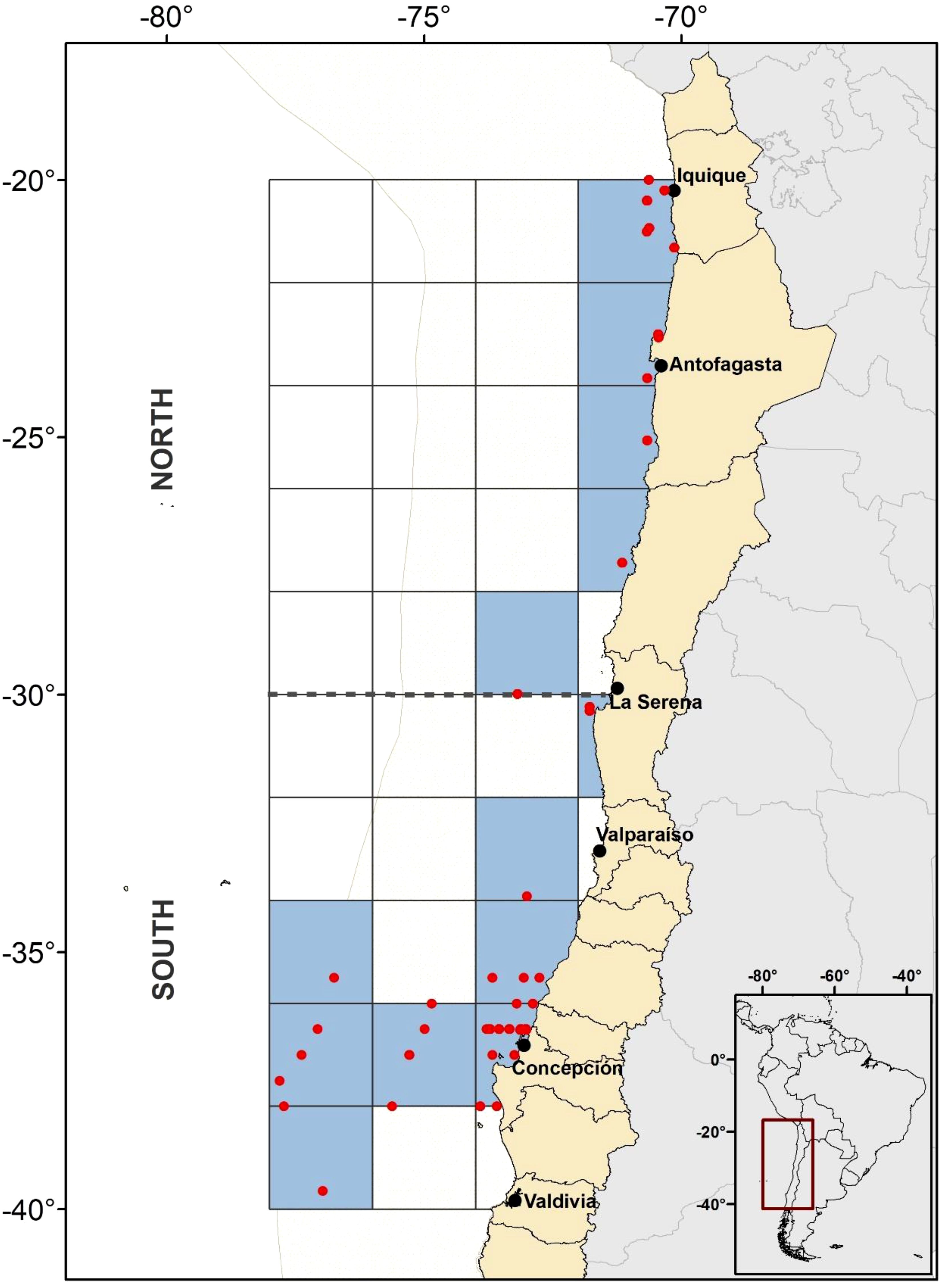
Figure 1. Study area at the Humboldt Current System (HCS, represented by the sand color dotted area) delimiting the 2x2 degrees cells forming the total grid. Blue grids represent the sampled ones, whereas the red dots represent the sampling stations from where data was obtained. The black dashed line at 30°S separates the north zone (NZ) and the south zone (SZ) of the HCS study area. The map projection is WGS 84 (EPSG 4326).

2.2 Data sources—Copepoda species and quality control procedures

Species occurrences were downloaded during August 2023 from the Ocean Biodiversity Information System (OBIS) database using its Mapper tool (https://mapper.obis.org/). The OBIS (Klein et al., 2019) is a global database of marine biodiversity and associated environmental data, which provides critical information to researchers and policymakers worldwide (Gan et al., 2023). OBIS is constructed from various institutions, projects and programs which may not necessarily apply common protocols for sampling. Detailed samplings are not mandatory for data suppliers and responsible people can be contacted using complementary information provided with data sets. The data were obtained by drawing a polygon surrounding the study area coupled with the filters “Copepoda” (taxonID 1080) for the Scientific name, selecting five strata of 100 m each between 500–0 m depth and within the time range from 1995 to 2011. Following the retrieval of the data, five.csv files were obtained with a sheet in Darwin Core format containing all copepod registers for that area, time and depth ranges, that were later depurated by eliminating occurrences without geographic coordinates, coordinates equal to zero, or those located inside the continent. We only selected occurrences at the species level and excluded duplicate records. This procedure allowed us to compile data to estimate species diversity indices, but also resulted in a reduction of information since many records are reported for genera or higher taxonomic levels (e.g. families), and in some cases without clear or wrong georeference. Taxonomy was revised and updated using the World Register of Marine Species (WoRMS) portal (http://www.marinespecies.org) through the match_taxa function of ‘robis’ package (Provoost and Bosch, 2021) implemented in R software (R Core Team, 2021). After we had cleaned and curated the data, a total of 7013 occurrence records of Copepoda species were selected, and the number of species was counted by bathymetric strata and latitudinal zones (Table 1). The data on occurrences of Copepoda species are available in a Zenodo repository: https://doi.org/10.5281/zenodo.15053910 (version 1).

Table 1

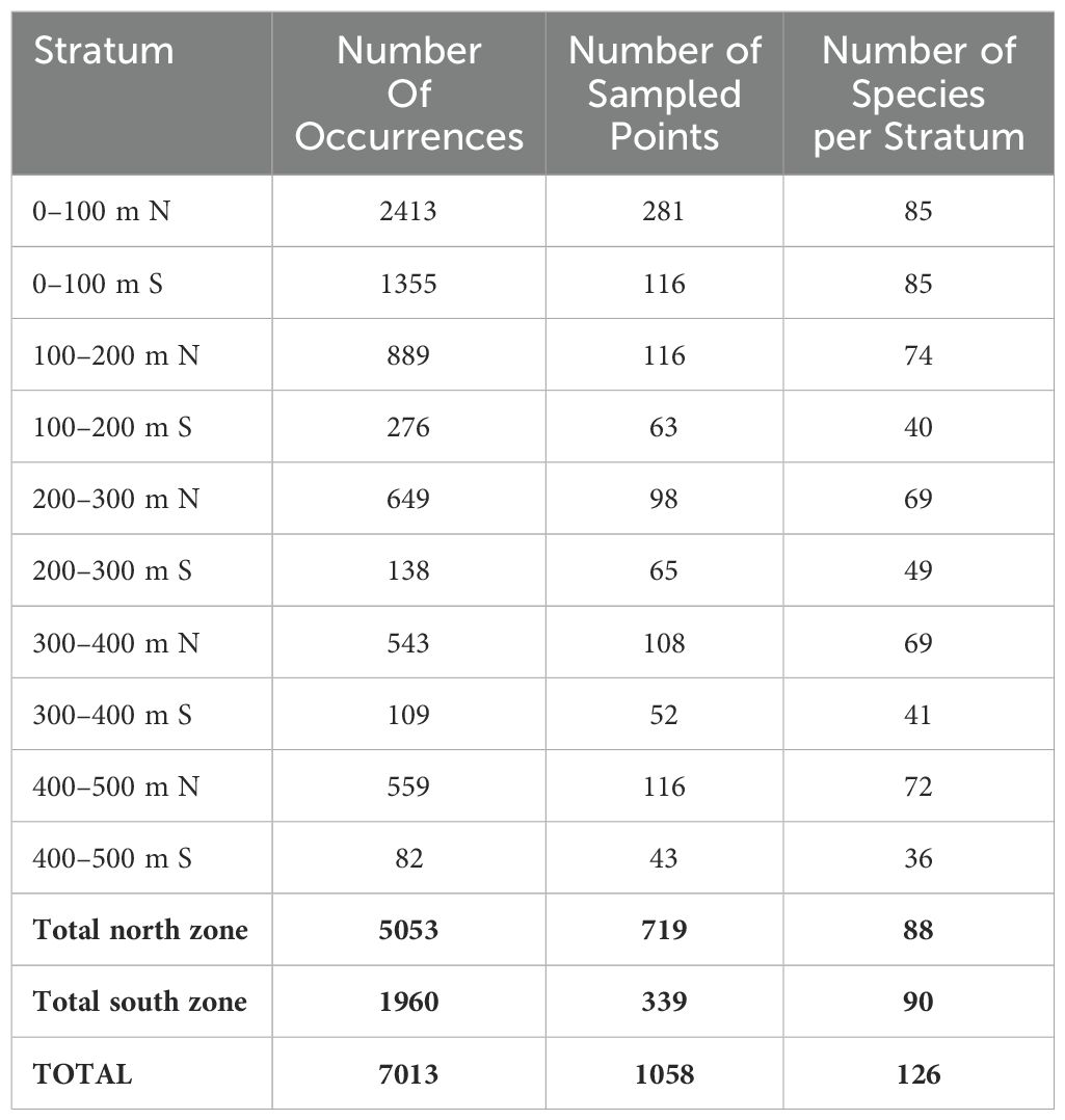
Table 1. Number of occurrence records at species level per strata and zone in the study area. N=north; S=south.

2.3 Data sources—environmental data

Eight oceanographic and two atmospheric variables were selected for the analysis. The oceanographic variables were obtained from Copernicus Marine Environment Monitoring Service (CMEMS, https://marine.copernicus.eu) to a resolution of 1 x 1 degree and 0.25 x 0.25 degrees, namely: mean temperature and mean salinity, from global ocean reanalyzes with data assimilation of satellite and in situ observations (Desportes et al., 2021); total chlorophyll-a concentration, dissolved oxygen concentration and pH from PISCES biogeochemical model forced by daily mean fields of ocean, sea ice and atmosphere coming from numerical simulation and reanalysis (Le Galloudec et al., 2021); geostrophic eastward sea water velocity (ugo) and geostrophic northward sea water velocity (vgo) from reprocessed in-situ and satellite data (Guinehut, 2021); and particulate organic carbon (POC) from reprocessed in-situ and satellite data (Sauzède et al., 2023). The atmospheric variables of eastward and northward components of the wind at a height of 10 meters above the surface of the Earth (u10 y v10, respectively) were obtained from the Copernicus Climate Change Service (C3S) Climate Data Store (CDS) to a resolution of 0.25 x 0.25 degrees from reanalysis combining model data and in situ observations (Hersbach et al., 2023). Monthly surface (10 m height) wind velocity was used to compute the alongshore wind speed climatology. For each latitude, standard deviation is also computed from the monthly alongshore wind series to assess the wind variability.

All variables were retrieved within the time range from 1995 to 2011, except POC—which registers start from 1998, and averaged between those years, as well as for each depth range both in the north and south zones of the study area (i.e., 0–100 m, 100–200 m, 200–300 m, 300–400 m, 400–500 m). They are available in a Zenodo repository: https://doi.org/10.5281/zenodo.15054097 (version 1).

To compute the Eddy Kinetic Energy (EKE), daily currents from the 1/12° horizontal resolution GLORYS12 reanalysis were downloaded from the CMEMS. Zonal and meridional current anomalies u’ and v’ were then computed from seasonal climatology. Finally, EKE is computed as (Jia et al., 2011):

EKE = \frac{1}{2} (u_{}^{'}_{g}^{2} + v_{}^{'}_{g}^{2})

Also, we tested environmental stability for temperature and salinity. The ‘environmental stability’ hypothesis (Pianka, 1966) posits that regions experiencing intense climate fluctuations are likely to exhibit lower biodiversity (Dynesius and Jansson, 2000; Zuloaga et al., 2019), whereas areas less impacted by extreme environmental events foster increased speciation, reduce extinction rates, and promote the accumulation of biodiversity (Dynesius and Jansson, 2000; Sandel et al., 2011). Then, to test the climate stability hypothesis and assess stability for each variable (temperature and salinity), deviation through time is calculated as the means of standard deviations between time slices divided by the time elapsed between time slices. The stability is then defined as the inverse of deviation through time, where the product of the estimates for each variable is rescaled between 0 and 1, here 0 indicates low and 1 indicates high stability (Owens and Guralnick, 2019). This analysis generates a raster showing the geographic distribution of climate deviation through time. The calculations were performed with the ‘climateStability’ package (Owens and Guralnick, 2019).

2.4 Data sources—processing

All species occurring in each stratum from each zone were compared to the total to determine the number of shared and non-shared species and then to determine exclusive (restricted range) and more widely distributed species. These features were analyzed in R software (R Core Team, 2021). The analysis was run by using the %in% operator and the union, intersect and setdiff functions that operate row-wise on data frames (in this case, lists of species as vectors for each stratum and zone). The script used for this analysis is available in a Zenodo repository: https://doi.org/10.5281/zenodo.15054153 (version 1).

All environmental variables were resampled to a resolution of 2 degrees (Figure 1) using QGIS 3.10 (QGIS Development Team, 2022). Initially, nine predictors were considered in our analyses (mean temperature, mean salinity, temperature stability, salinity stability, total chlorophyll-a concentration, dissolved oxygen concentration, pH, particulate organic carbon (POC), and EKE. Then, we obtained the Spearman rank-order correlation coefficient matrix with the ‘corrplot’ package (Wei and Simko, 2024), for visualizing their degree of association. Predictors showing correlation values over 0.7 were removed for further analyses (Dormann et al., 2013); then, particulate organic carbon (POC) and pH were no longer considered (Supplementary Figure S1). The remaining predictors were later used to evaluate species richness, the Shannon-Wiener index, the Hurlbert index, and β-diversity and its additive components: turnover, and nestedness (eg., Baselga, 2010; Baselga and Gómez-Rodríguez, 2019).

2.5 Diversity estimates

We calculated alpha diversity as species richness and beta diversity as species composition. In the latter, we differentiated between turnover and nestedness. Alpha diversity was calculated in Biodiverse 3.1 software (Laffan et al., 2010), whereas beta diversity was estimated using the packages ‘betapart’ (Baselga and Orme, 2012), ‘CommEcol’ (Sanches Melo, 2021) and ‘letsR’ (Vilela and Villalobos, 2015) using the following equation:

β s o r = β s i m + β s n e \equiv \frac{b + c}{2 a + b + c} = \frac{b}{b + a} + (\frac{c - b}{2 a + b + c}) (\frac{a}{b + a})

where βsor is Sørensen dissimilarity, βsim is Simpson dissimilarity (i.e., turnover component of Sørensen dissimilarity), βsne is the nestedness component of Sørensen dissimilarity, a is the number of shared species between two cells, b the number of species unique to the poorest site, and c the number of species unique to the richest site.

The Hulbert diversity index was also calculated, and although it is designed to measure dominance in a community, where a lower value indicates greater diversity and a higher value indicates greater dominance, it can be used for presence-absence data, calculating the proportion of sample units where that species is present. To do this, count the number of sample units with the presence of the species and divide by the total number of sample units, as follows:

H = 1 - \frac{1}{N} \sum_{i = 1}^{S} p_{i}^{2}

where:

● H is the Hulbert diversity index,

● N is the total number of sample units,

● p_i is the proportion of presence of species i in the sample units and

● S is the total number of species.

The calculations were performed with the ‘vegan’ package (Oksanen et al., 2024), and the script is available in the Zenodo repository: https://doi.org/10.5281/zenodo.15054153 (version 1).

Since we only have occurrence records, the Shannon-Wiener index was calculated considering that each species present has the same importance in the community. In this case, the proportions 𝑝i𝑖 will be defined as the proportion of species present with respect to the total species in the set. Then, the Shannon-Wiener index for occurrence data was calculated in Biodiverse 3.1 software (Laffan et al., 2010), according to Laffan (2022):

H = - \sum_{i = 1}^{n} p_{i} \cdot l n p_{i}

where p_i is the number of samples (in this case, occurrences) of the i species as a proportion of the total number of occurrences in the neighborhoods (2° x 2° sampling cells). This proportion is estimated as:

p_{i} = \frac{n_{i}}{N}

where n_i is the number of records of the i species and N is the total number of records at species level in the sampled cell.

For species richness, spatial hotspots were defined using spatial clustering analysis, Getis-Ord G* statistic (Getis and Ord, 1992). This identifies spatial concentrations of an entity (in this case species richness per cell) or areas that contain higher/lower values than expected by chance for a given study area. Significant values of Z>0 provide evidence for significant hotspots whereas values of Z<0 provide evidence for groups of entities with lower values than expected by chance. The statistical determination of hotspots was performed in ArcMap 10.4.1 software (ArcMap™ by Esri® software, 2016) and were plotted by using the package ‘ggridges’ (Wilke, 2024).

2.6 Statistical analysis

To evaluate differences in diversity and richness between strata, as well as between NZ and SZ, we used a two-way Permutational Multivariate Analysis of Variance (PERMANOVA) (Anderson, 2001) since statistical inferences are made in a distribution-free setting using permutational algorithms (Anderson, 2001, 2017). This analysis was performed in PAST v 4.17 software (Hammer et al., 2001).

To assess the effect of the environmental variables on diversity, Linear Mixed Models (LMM) were used, which allow both fixed and random effects, thus serving for analyzing data that are non-independent (Arnqvist, 2020; Bates, 2005; Bolker, 2015). First, we assessed normality using Shapiro-Wilk test. This analysis showed that species richness (W = 0.85695; p-value = 2.399e-05), Shannon index (W = 0.8206; p-value = 2.707e-06), Hurlbert index (W = 0.85695; p-value = 2.399e-05), β-diversity (W = 0.82175, p-value = 2.888e-06), and its additive components: turnover (W = 0.95377, p-value = 0.04883) and nestedness (W= 0.79035, p-value = 5.292e-07) had normal distribution. Then, a set of Linear Models (LM) and Linear Mixed Models (LMM) were developed for species richness, the Shannon-Wiener and Hurlbert indices, β-diversity and its two additive components: turnover, and nestedness. The residual diagnosis was carried out using the simulateResiduals function in ‘DHARMa’ package (Hartig, 2024) to assess the distribution of data and their independence through observing the dispersion in variance. A lack of independence in the data can lead to overdispersion, which can be accounted for by fitting a random effect on the model. The residuals diagnosis showed that residuals for Linear Models (LM) and Linear Mixed Models (LMM) showed no deviation from the expected normal distribution (Supplementary Figure S2, left panel), and that the difference between the observed and expected values was greater in the LM (i.e., they showed more unexplained variation of their residuals shown as an over-dispersion in their variance, Supplementary Figure S2, right panel). Then, the analyses continued with the use of LMM, that included mean temperature, temperature stability, mean salinity, salinity stability, chlorophyll-a concentration, oxygen concentration, and EKE as fixed-effect predictors, whereas bathymetry (every 100 m strata) and zones (north and south) were included as random effects. These analyses were performed with the ‘lme4’ package (Bates et al., 2024). The environmental variables were normalized before the analysis. We generated a series of models to evaluate the drivers of diversity (Supplementary Table S3); the models with the best fit were selected through the corrected Akaike Information Criterion (AICc), through the ‘MuMIn’ package (Bartoń, 2022). Models with ΔAICc values (i.e., the difference in AICc score between the best model and the model being compared), within 2 units of the best model should be selected (Anderson et al., 2008). Finally, a marginal and conditional R² value was estimated for the best models with the r.squaredGLMM function of ‘MuMIn’ package (Bartoń, 2022). The marginal R² (R²m) estimates the fraction of the variance explained by the fixed effects in the model, whereas the conditional R² (R²c) estimates the fraction explained by the fixed and random effects. The script of this analysis is available in the Zenodo repository: https://doi.org/10.5281/zenodo.15054153 (version 1).

3 Results

3.1 Spatial biodiversity

Each stratum at the northern and southern zones (NZ and SZ, respectively), as well as the integration of strata per zone and for the whole study area, showed spatial biodiversity patterns that are summarized in Supplementary Figures S4, S5 and Supplementary Tables S1a,b and S2 (Supplementary Material). Only 18 species are common to all strata, thus distributed from 0 to 500 m at the NZ and SZ of the study area (Supplementary Table S2 Supplemental Material): Agetus typicus, Calanoides patagoniensis, Calanus chilensis, Euchaeta marina, Heterorhabdus papilliger, Metridia brevicauda, Metridia lucens, Oithona plumifera, Oithona setigera, Oithona similis, Oncaea curvata, Oncaea media, Oncaea mediterranea, Paracalanus indicus, Pleuromamma gracilis, Pleuromamma quadrungulata, Triconia conifera, and Triconia minuta. There are 46 common species at the NS and SZ of the 0–100 m stratum (Supplementary Figure S4 and Supplementary Table S2), whereas the 100–200 m, 200–300 m, 300–400 m, and the 400–500 m strata have 26, 29, 28, and 23 common species from the NS and SZ, respectively (Supplementary Table S2).

We found that the NZ and SZ have 32 and 14 exclusive species, respectively (Supplementary Table S1a and S2). This means that those species can only be found at the north or south zone, at different strata. Regarding exclusive species per zone and stratum, only three strata had species that were not repeated elsewhere within the study area: 0–100 m NZ, 0–100 m SZ and 400–500 m NZ. Four species were exclusively registered at the 0–100 m NZ stratum (Supplementary Table S2), twenty-five species were exclusively registered at the 0–100 m SZ (Supplementary Table S2), and two species were exclusively registered at the 400–500 m NZ stratum (Supplementary Table S2).

From the common species for the north and south zone that occur along all strata (Supplementary Table S2) the order Cyclopoida and Calanoida both present 50% relative occurrence, with nine species each (Table 2). From the order Cyclopoida, the family Oncaidae showed the greatest number of representatives (five species), followed by Oithonidae (three species) and Corycaeidae (one species) (Table 2). From the order Calanoida, four species belong to the Metridinidae family, two species to the Calanidae family, and one species to the Euchaetidae, Heterorhabdidae, and Paracalanidae families, respectively (Table 2). The observed distribution of these species occurrences at this study have been previously cited off Chile (Table 2).

Table 2

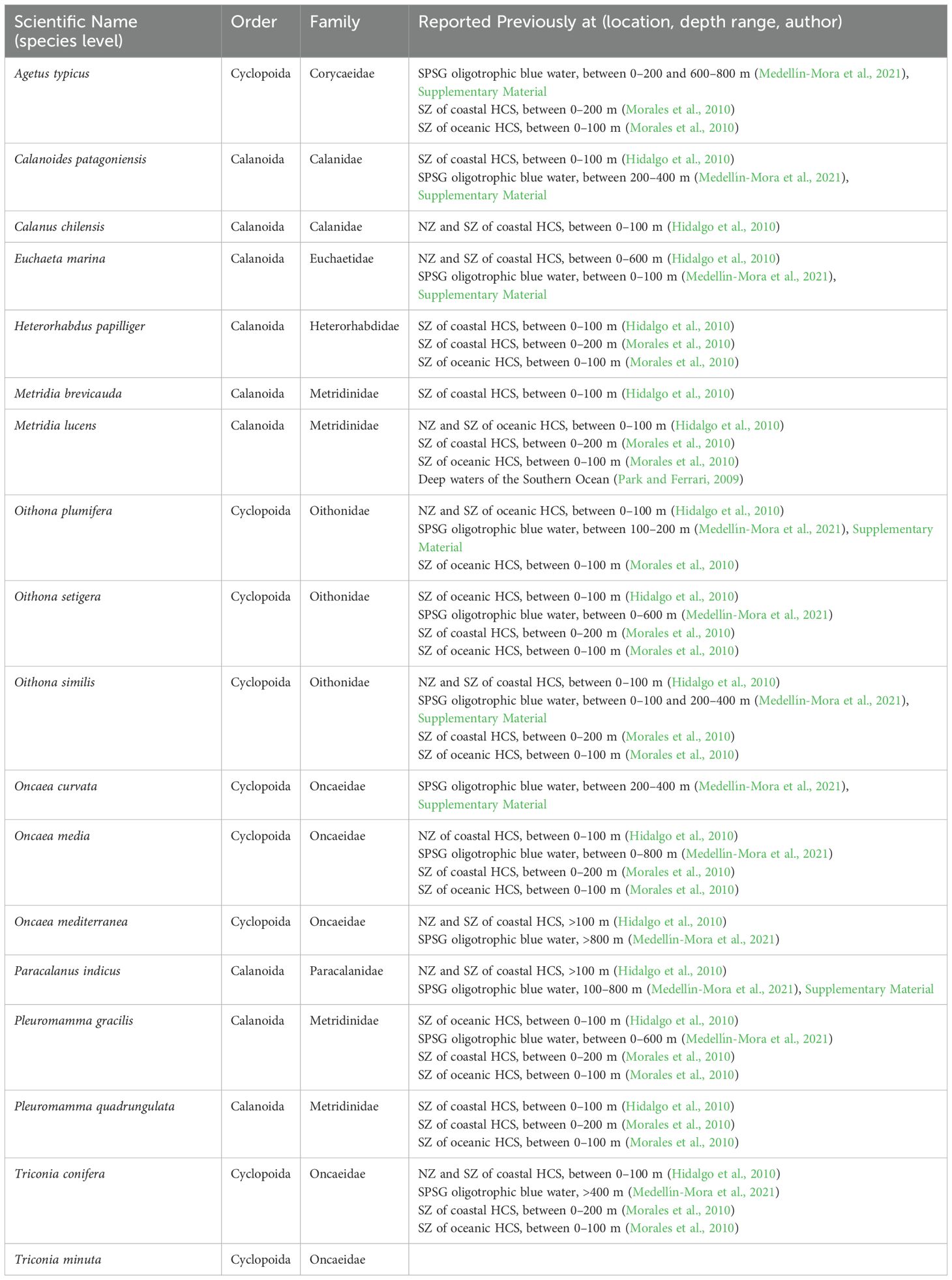
Table 2. Dominant species of the HCS off Chile, occurring between 0 and 500 m depth and between 20°-40°S and 70°-78°S.

3.2 Environmental stability

The Hovmöller diagram of the alongshore winds’ climatology showed that there is seasonal upwelling south of 35°S, whereas north of this latitude upwelling is continuous (Figure 2a). Regarding wind’s variability, its monthly standard deviation is greater towards the south (Figure 2b).

Figure 2

(a) Heat map showing alongshore wind intensity from January to December between latitudes 20 and 40 degrees south. Colors range from blue (low intensity) to red (high intensity). (b) Line graph depicting the standard deviation of monthly alongshore wind, measured in meters per second, across the same latitudes. The trend shows a decrease in standard deviation with decreasing latitude.

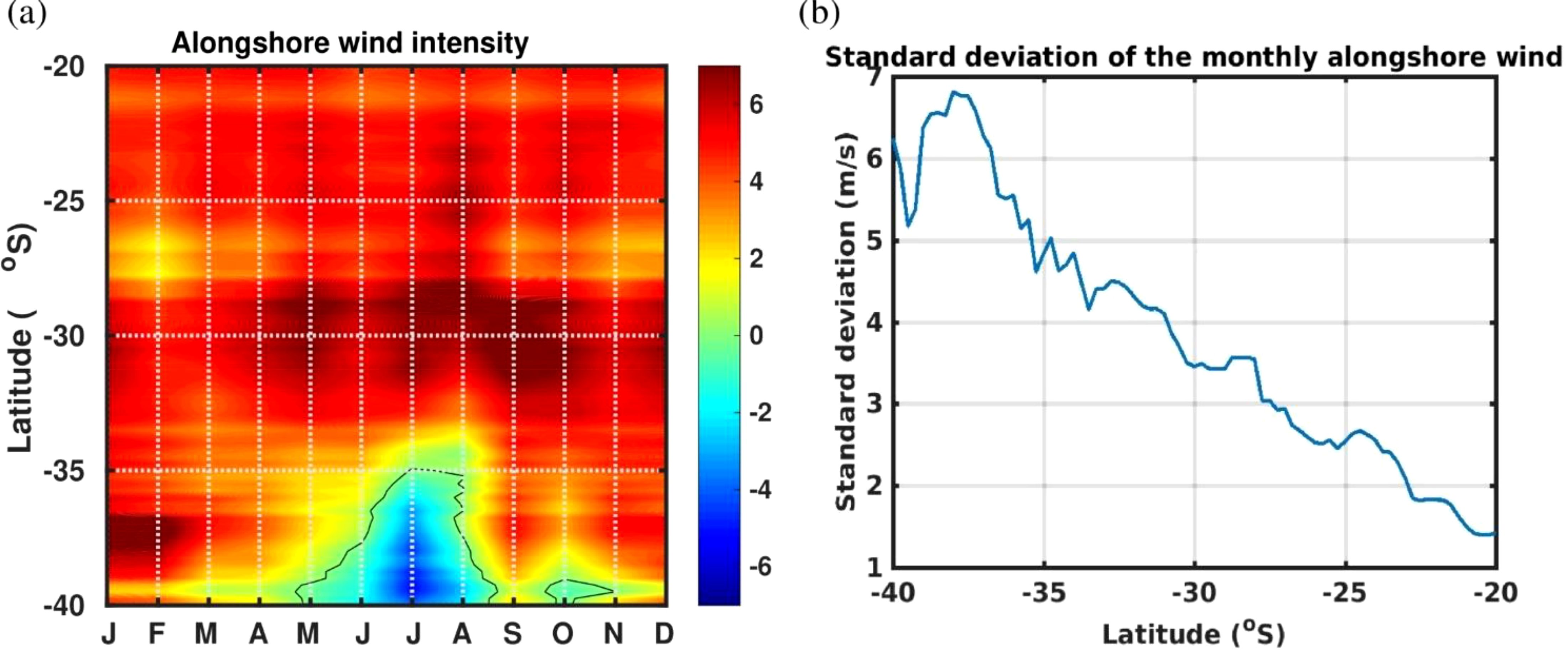
Figure 2. Alongshore surface wind speed (in m s^-1) from ERA5 reanalysis over the 1995–2011 period (a) Hovmöller diagram of the wind speed monthly climatology (b) latitudinal variation of the monthly wind standard deviation.

The turbulent kinetic energy at the surface analysis showed a zone with maximum EKE between 26 and 36°S (Figure 3a, detail in Supplementary Figure S3), whereas the vertical EKE profiles averaged for each zone shows that NZ has a more intense mesoscale activity compared to the SZ (Figure 3b). For better assessing EKE latitudinal variations, it was averaged into 1° latitude band and plotted along the strata, where it shows maximum intensity between 26 and 34°S over 100 m depth, decreasing with depth at all latitudes, and with a stronger decrease in the upper layers in the SZ than in the NZ (Figure 3c).

Figure 3

Figure 3. Mean Eddy Kinetic Energy (EKE in cm²; s^-2;) computed from the daily outputs of the Glorys12 reanalysis over the 1995–2011 period. (a) surface EKE (b) vertical profile of the mean EKE averaged over the 20-30°S region (blue line) and the 30-40°S region (red line) (c) latitudinal variation of the mean EKE averaged from the coast to 78°W and over 1° latitudinal bins, at different depths (0, 50, 100, 200, 300, 400 and 500 m).

3.3 Statistical outcomes

The two-way PERMANOVA analyses showed that species richness and Shannon-Wiener index were significantly different between zones, but not between strata (Table 3). These diversity measures showed that, on average, NZ had higher species richness and a Shannon-Wiener index in all strata, excepting the 300–400 m depth range (Figures 4B, F, respectively). On the other hand, nestedness was significantly different between strata but not between zones (Table 3), indicating greater mean differences in the 100–200 m and the 200–300 m depth ranges, and lower mean differences in the 0-100m, 300–400 m, and 400–500 m depth ranges (Figure 4E). Hurlbert index, species composition and turnover were significantly different between zones, as well as between strata (Table 4). In particular, the Hurlbert index was on average greater in the NZ and upper strata (0–100 m, 100–200 m, and 200–300 m depth ranges; Figure 4D); whereas the species composition and turnover were on average greater in the NZ and lower strata (100–200 m, 200–300 m, 300–400 m and 400–500 m depth ranges; Figures 4A, C, respectively).

Table 3

Table 3. Two-way PERMANOVA results for models of species richness, Shannon-Wiener index, Hulbert index, species composition and its components turnover and nestedness.

Figure 4

Six line graphs labeled A to F, each showing relationships between depth in meters and different diversity indices. Orange lines represent NZ, and blue lines represent SZ. Graphs depict metrics: A) Beta, B) Alfa, C) Turnover, D) Hurlbert, E) Nestedness, F) Shannon, with varying trends across depths from 0-500 meters.

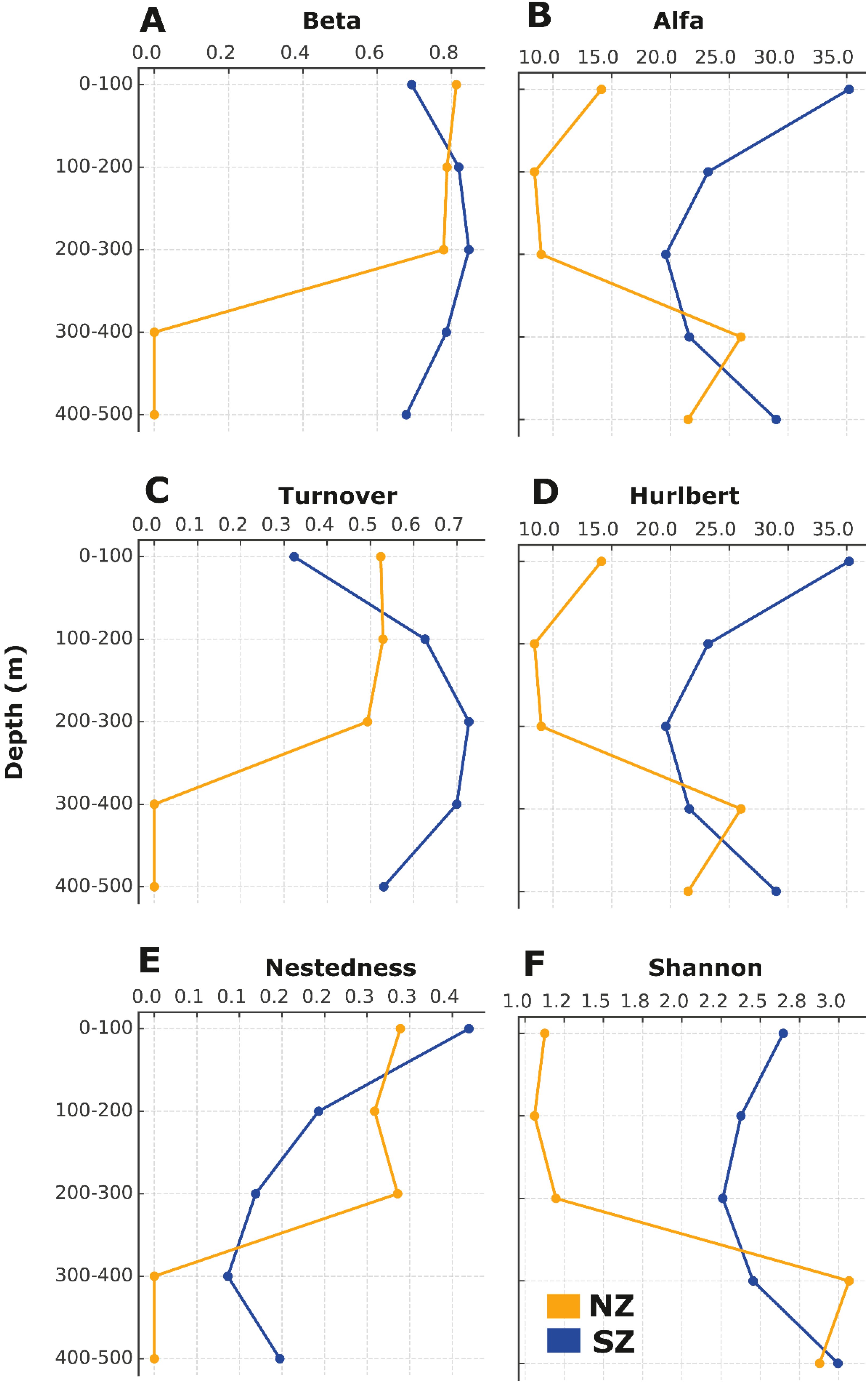
Figure 4. Diversity indices for (A) beta diversity, (B) alfa diversity, (C) turnover component of beta diversity, (D) Hurlbert index, (E) nestedness component of beta diversity, and F) Shannon-Wiener index in the study area, separated by zone (NZ=north zone, orange lines; SZ=south zone, blue lines) and bathymetric range (from 0 to 500 m depth).

Table 4

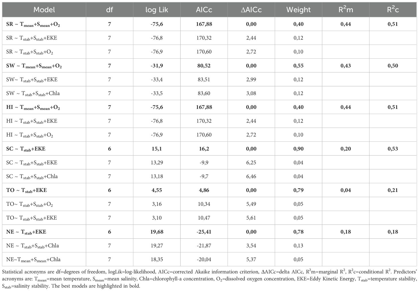
Table 4. LMM for species richness (SR), Shannon-Wiener index (SW), Hurlbert index (HI), species composition (SC) and its components turnover (TO) and nestedness (NE).

The clustering analysis (Getis-Ord Gi*) allowed us to identify high values of richness in all strata at NZ, whereas cold spots (i.e., low species richness values) were greater at SZ and at greater depths (Figure 5).

Figure 5

Density plots illustrate Z-score distributions for North and South zones across five bathymetric ranges: 0-100m, 100-200m, 200-300m, 300-400m, and 400-500m. North data is orange, South is blue.

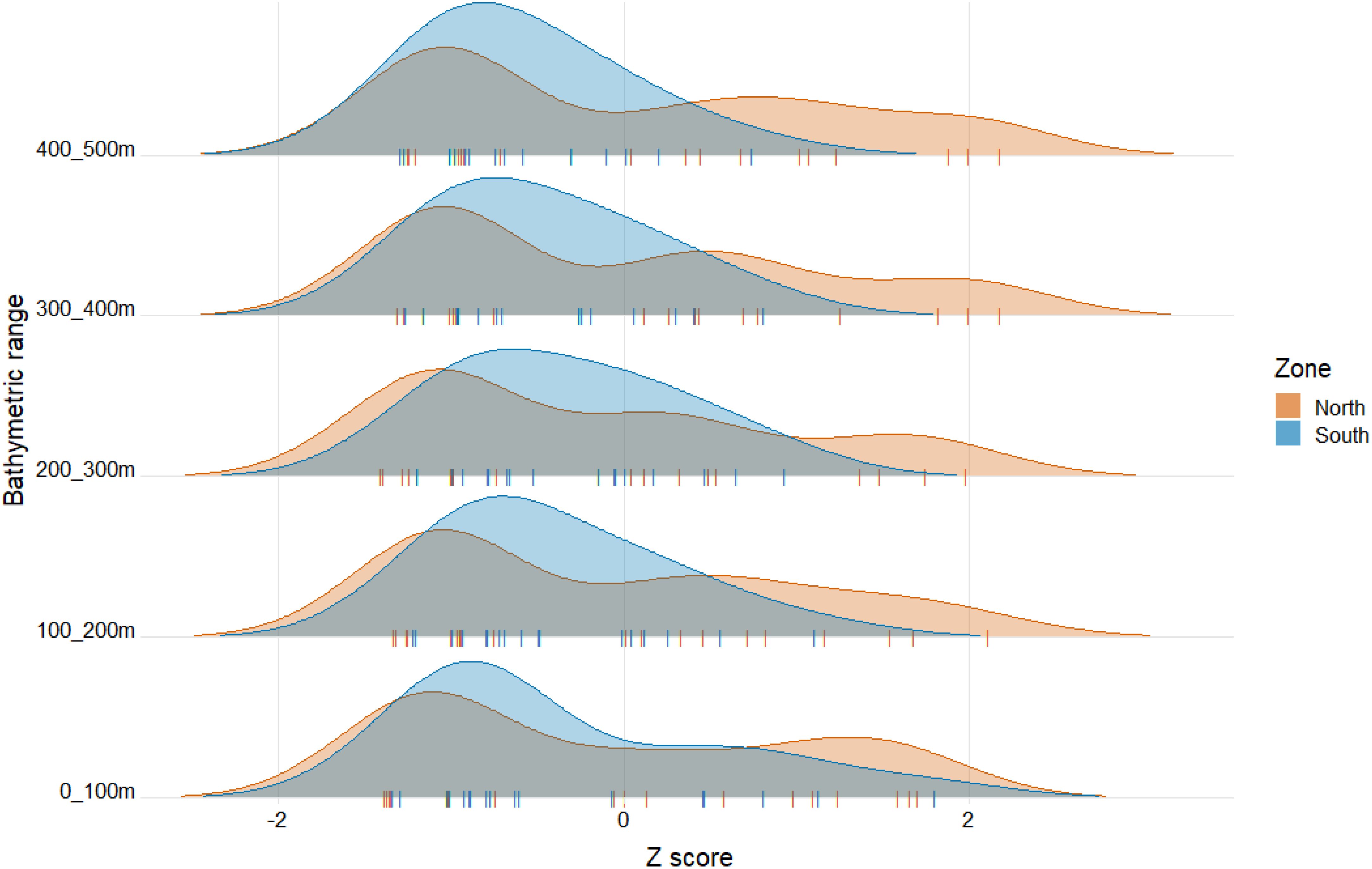
Figure 5. Getis-Ord Gi* statistic of species richness of Copepoda at each depth range and zone of the study area. A positive value for a standardized Z score suggests a hot spot, whereas a negative value indicates a cold spot.

The best-fitting LMM explaining species richness revealed that the variables mean temperature, mean salinity, and oxygen concentration were the most important predictors (Table 4). The R²m and the R²c explain 44% and 51% of the variability, respectively. The environmental predictors that explain the diversity evaluated through the Shannon-Wiener index included mean temperature, mean salinity, and oxygen concentration (Table 4). The R²m and the R²c explain a 43% and a 50% of the variability, respectively. The best-fitting model for diversity assessed through the Hurlbert index indicated that temperature, mean salinity, and oxygen concentration were significant predictors (Table 4). The R²m and the R²c explain 44% and 51% of the variability, respectively. The environmental predictors explaining the distribution of beta diversity (species composition), included temperature stability and EKE (Table 4). The R²m and the R²c explain a 20% and a 53% of the variability, respectively. The environmental predictors that explain the distribution of turnover included temperature stability and EKE (Table 4). The R²m and the R²c explain a 4% and a 21% of the variability, respectively. The environmental drivers that explain the distribution of nestedness included temperature stability and EKE (Table 4). Both the R²m and the R²c explained 18% of the variability.

4 Discussion

The assessment of copepod diversity patterns in the HCS both, over the horizontal and vertical planes, clearly indicated a strong connection between the copepod community and upwelling variation. Changes in upwelling intensity over a seasonal time scale and according to the latitudinal regime can strongly influence the habitat conditions for copepods inhabiting the upper 500 m in the HCS. These changes can affect copepod populations and ultimately the community structure, including biodiversity. It is also important to highlight the strong link between the diversity indices and environmental stability as assessed by temperature stability and kinetic energy (EKE). It has been documented that habitat stability modulates biodiversity along time (Navarro-Mayoral et al., 2024), and that climate change-induced modifications of the mechanisms sustaining ecological stability can result in taxa richness reduction and overall ecosystem malfunctioning (Wang et al., 2023). Then, more stable conditions throughout the year can allow populations to reproduce more continuously and so be present permanently, but also this stability may help maintaining the community composition more stable year-round. In this context, it can be inferred that fewer perturbations or a more predictable environment may also allow that species interactions along with their specific responses to environmental change can function more efficiently (Fischer et al., 2001) to promote a higher species richness.

It is important to stress that both temperature stability and EKE are driven by variation of upwelling intensity. Regarding latitudinal variation, it must be noted that permanent continuous upwelling regime north of 35°S derived from alongshore winds’ climatology (Figure 2a) and greater surface EKE (Figure 3a) are masked by the delimitation of the zones for this study, as the southern region (SZ) starts at 30°S. However, when considering averages for each zone, a lower monthly standard deviation of wind’s variability (Figure 2b) together with greater EKE along depth (Figures 3) can be observed in the northern region (NZ) than in the SZ, indicating more upwelling favorable conditions in the NZ throughout the year, while the SZ shows more variability between seasons, giving lower average values. On the other hand, it has been documented that the SZ (data from 36,4°S) is characterized by a continuous alternation between strong southerly and weak northerlies (UI < 0, downwelling favorable), even at a sub-seasonal scale (Aguirre et al., 2021), with implications on biogeochemical cycles and productivity. In addition, a more poleward location of the South Pacific High during winter has caused more summer-like hydrographic conditions on the continental shelf offshore central Chile (where the SZ was delimited), generating changes in the plankton community (Jacob et al., 2018; Schneider et al., 2017) that may explain increased coastal upwelling in the HCS, and the changes in species dominance associated with it in terms of abundance (Pino-Pinuer et al., 2014), as shifts in the upwelling regimes also affects phytoplankton composition that in turn are determinant for zooplankton reproductive pulses (Vargas et al., 2006). Besides that, wind-forced upwelling can transport naturally occurring low dissolved oxygen waters towards the continental shelf and even cause mortality of different species (Roegner et al., 2011). At the HCS, NZ is characterized by an oxygen minimum zone that is relatively shallow (ca. 10–60 m depth of its upper limit) (Hidalgo et al., 2005; Morales et al., 1999) in the coastal upwelling area and adjacent oceanic waters, generating usually low oxygen concentrations to which organisms may respond in physiological or distributional terms (Morales et al., 1999; Gilly et al., 2012). Despite zooplankton may tend to aggregate above the oxycline associated with more oxygenated surface waters (Tutasi and Escribano, 2020), nauplii, small- and large-sized copepods are able to perform diel vertical migration through the upwelling zone, withstanding severe hypoxia and being able to exhibit a large migration amplitude (∼500 m, large-sized copepods and copepods of the group Eucalanidae), remaining either temporarily or permanently during day or night conditions within the core of the OMZ (Tutasi and Escribano, 2020). Therefore, considering that the OMZ occurs over the whole study area under different conditions and reaches depths of ca. 500 m, it appears that the dominant species described here in terms of occurrence for the HCS (scientific names detailed in Tables 2 and S2) may be adapted or have evolved the capacity to cope with low oxygen conditions, temporally through vertical migration (Tutasi and Escribano, 2020) or during more extended periods (Hidalgo et al., 2005). This also could explain the fewer exclusive species found in the 0–100 m depth range at NZ (Supplementary Table S2), as different species may occur along the whole water column, whereas at the SZ more species may tend to aggregate in the upper layer for oxygen (Tutasi and Escribano, 2020) or when the OMZ becomes shallower. The clustering analysis (Figure 5) indicated a similar tendency, with high values of richness in all strata at the north zone (NZ), whereas low species richness values (cold spots) were found at greater depths in the south zone (SZ).

Regarding copepod species diversity, the species common to all strata and zones (Tables 2 and S2) can be considered, in terms of occurrence, dominant for the HCS off Chile as they occur between 0 and 500 m depth and between 20°-40°S. The observed distribution of these species occurrences at this study have been previously cited off Chile (Table 2), and corroborates, complements or broadens the information previously documented.

From the dominant species of the HCS, Calanus chilensis has been considered as a coastal-neritic species endemic to the eastern South Pacific between 10° and 42°S (Marín et al., 1994), highly adapted to the environmental condition of the HCS (Escribano, 1998), and being later proposed as a biological indicator of the intrusion of the Humboldt Current in the Ecuadorian Pacific (Bucheli et al., 2019). More recently, a continuous distribution for the species has been modeled, that ranges from Ecuador to the southernmost area of South America between 0–200 m depth range, whereas the organisms occurring between 200–400 m have a modeled discontinuous distribution with greater suitability for the coast of Chile (Rivera et al., 2023). The neritic zone comprises the shallow coastal waters (down to 100–200 m) overlying the continental shelf (Boaden and Seed, 1985); however, in this study the occurrence of C. chilensis has been registered down to a depth of 500 m, supporting the modeled projection of this species. Together with C. chilensis, Calanus patagoniensis is another species considered endemic to the HCS, but with a more inshore distribution due to biological behavior involving vertical migration that may avoid them to be transported offshore by mesoscale processes (Morales et al., 2010). When revising our data, we can corroborate that for the south zone, that has more data available towards open ocean, C. chilensis occurs along all its extension, while C. patagoniensis occurrences are restricted until the 73°W centroid. Oithona similis, Paracalanus indicus, Pleuromamma gracilis and P. quadrungulata are species that we found to be dominant in terms of occurrence and that have been described in other studies as dominant for the HCS (Escribano et al., 2012; Pino-Pinuer et al., 2014). Here, we found these species occurrence to be restricted until the 73°W centroid as well. P. indicus dominance in terms of abundance has been documented to vary strongly over the south zone, being outnumbered by Drepanopus forcipatus (Pino-Pinuer et al., 2014). In this study, D. forcipatus did not appear to be dominant in terms of occurrence as it only appeared between 0–200 m at NZ and SZ (Supplementary Table S2), and restricted until the 73°W centroid, which is concordant with its known distribution restricted to coastal and shelf areas along southern South America (Park and Ferrari, 2009). Additionally, it has been reported that the regional distribution of C. chilensis secondary production extends much further offshore in the HCS than what is typical for its ecological counterparts in other coastal upwelling systems, extending the area of high productivity which in turn maximizes trophic transfer efficiency towards economically important pelagic fish (Schukat et al., 2021). These aspects involve specific life-strategy traits and life-cycle adaptations (Schukat et al., 2021) that highlights C. chilensis importance as an endemic species adapted to the environmental variability of the HCS.

Acartia tonsa is a widely studied species in the HCS (e.g., Aguilera, 2020; Aguilera and Bednaršek, 2022; Ruz et al., 2015; Yáñez et al., 2018), considered cosmopolitan and characteristic of estuarine and upwelling systems, while also associated to the inshore area (Morales et al., 2010). In this study, this species did not appear to be dominant for the HCS, however it is present in both NZ and SZ between 0–300 m (Supplementary Table S2) and restricted until the 73°W centroid, thus it may be considered an upper-mesopelagic species.

Paraeuchaeta barbata appeared as an exclusive species for the 400–500 m stratum of the NZ (Supplementary Table S2). This calanoid species occurs in deep water throughout the world oceans (Park, 1994), being a very common species between the Southern Ocean and the Arctic basin (Park and Ferrari, 2009) associated with the Antarctic Intermediate Water (AAIW) during austral summer and winter when migrating from and arriving to the Chilean coast, respectively (Yamanaka, 1976). This demonstrates that vertical zonation occurs in the HCS and is associated with seasonal physical-biological processes that in turn may be linked to temperature. Moreover, various species found in the HCS are characteristic of the Southern Ocean (SO) (Park and Ferrari, 2009), such as Metridia lucens and Pleuromamma quadrungulata, deep water species in the SO considered dominant species in this study (found between 0–500 m depth and in both the NZ and SZ, Table 2); Gaetanus brevispinus, G. kruppii, Lophothrix frontalis (deep water species in the SO), Metridia gerlachei (very common herbivore calanoid in the SO), found between 0–500 m in the NZ in this study (Supplementary Table S2); Calanus propinquus, Neocalanus tonsus. (epipelagic calanoids of the SO, the latter can perform diapause), Gaetanus tenuispinus (very common deepwater species in the SO), found between 0–500 in the SZ in this study (Supplementary Table S2); Haloptilus oxycephalus, Scolecithricella minor (very common deepwater calanoids of the SO that reach temperate and subarctic regions, respectively), Ctenocalanus citer (epipelagic calanoid endemic to the SO) found between 0–100 m in the SZ in this study (Supplementary Table S2). These examples indicate intrusion and colonization of epipelagic and deepwater copepods from the SO, that are adapted to that productive habitat (Park and Ferrari, 2009), into the HCS. Thus, the HCS must be a suitable habitat for increasing regional diversity, especially that of calanoid copepods.

Generally, when several models produce quite similar AICc values (i.e., within 1 to 2 units of each other), it suggests that there is a reasonable amount of redundancy among predictor variables, as several different combinations of them could be used interchangeably to explain the observed relationship (Anderson et al., 2008). In this study, this was not the case (Table 4), so it can be inferred that the predictors are not inter-correlated. The fact that mean temperature, mean salinity, and oxygen concentration are the main predictors for richness indices such as alpha diversity, Shannon-Wiener index and Hurlbert index relates to the kinetic energy and the environmental stress hypotheses, as higher temperatures are beneficial for ectotherms development, which may lead to higher speciation rates (Fraser and Currie, 1996; Tittensor et al., 2010); whereas environmental stress in terms of temperature and salinity extremes (Fraser and Currie, 1996; Brucet et al., 2009; Hamil et al., 2020; Yuan et al., 2020; Jiménez-Melero et al., 2023) and oxygen depletion (Tittensor et al., 2010) is negatively correlated with diversity. This also reflects the relevance that water masses and the OMZ may have on copepod populations, as the environmental conditions they generate have effects on different aspects of copepods ecology in the HCS (Escribano et al., 2014; Ruz et al., 2018). The importance of temperature stability and EKE as main predictors of species composition and its additive components turnover and nestedness, relates to the climate stability and historical factors hypotheses, that assumes higher diversity in more environmentally stable regions (Tittensor et al., 2010) and provide habitat features that favor extant patterns of dispersal and richness (Fraser and Currie, 1996), respectively. Therefore, mesoscale activity seems to be an important feature at a regional scale for zooplankton, as it has been documented how copepods are transported offshore by eddies, with some species potentially coupling their ontogeny to that process, such as Calanus chilensis (Schukat et al., 2021).

Nevertheless, despite our results exhibiting different patterns between zones and strata for the HCS, we may find a potential limitation for studying biogeographic patterns in this area due to the lack of occurrence data for certain regions, that together with the fact that information is derived from different sampling methods, sampling gears and protocols of analysis, may restrict our understanding of the patterns and processes driving copepod diversity in the HCS. However, future research utilizing species distribution models (SDM) could help mitigate these data gaps.

In summary, it appears that even at regional scale, different aspects related to basal hydrographic conditions, as well as the coupling of physical and biological processes are affecting diversity, with responses to their variations in terms of phenotypic plasticity that are species-specific. This, added to the individual variability (Bi and Liu, 2017), may generate a variety of responses on copepod species. Moreover, within the context of climate change and global warming, it has been described that the effects of temperature variation on different marine communities at different scales are translated into a slowly replacement of cold-tolerant species with warm-tolerant counterparts, with the former being redistributed to greater depths (Burrows et al., 2019), without necessarily decreasing the system’s functionality or shifting horizontal patterns, unless the species interact with the surface for the need of light, or as in the case of copepods, for feeding following DVM. Then, some increased depth range found in this study for some copepod species may be related to warming responses and vertical redistribution. However, this may represent an increase in the metabolic activity for some individuals not adapted for low oxygen conditions or that perform their life cycles associated with processes occurring at shallower depths. Considering the dynamism of the HCS and the increased capacity of plankton to rapidly respond to environmental shifts in temporal and special scales, greater assessments are required for better understanding copepods distribution and their shifts extent, with an associated need for an enrichment of ecological data bases in terms of temporal and spatial coverage, for better implementing macroecological modeling techniques that yield more robust spatial patterns and their associated dominant drivers or processes.

Data availability statement

The original contributions presented in the study are included in the article/Supplementary Material. Further inquiries can be directed to the corresponding author/s.

Ethics statement

The manuscript presents research on animals that do not require ethical approval for their study.

Author contributions

MP-A: Conceptualization, Formal analysis, Investigation, Methodology, Writing – original draft, Writing – review & editing. RR: Conceptualization, Formal analysis, Investigation, Methodology, Software, Validation, Writing – review & editing. VO: Formal analysis, Methodology, Software, Validation, Writing – review & editing. CG: Formal analysis, Investigation, Methodology, Software, Validation, Writing – review & editing. CH: Conceptualization, Supervision, Validation, Writing – review & editing. RE: Conceptualization, Funding acquisition, Investigation, Resources, Supervision, Validation, Visualization, Writing – original draft, Writing – review & editing.

Funding

The author(s) declare that financial support was received for the research and/or publication of this article. This work was funded by the Instituto Milenio de Oceanografı́a (IMO) through the Agencia Nacional de Investigación Cientı́fica y Tecnológica de Chile (ANID) Grant AIM23-0003. CEH research is funded by ANID/FONDECYT 1201506, 1220998 and 1240219 Projects. The funders had no role in study design, data collection and analysis, decision to publish, or preparation of the manuscript.

Acknowledgments

We are grateful to all the scientific community providing data on marine biodiversity to OBIS portal, and especially thankful to Unesco/IODE/OBIS/ESPOBIS, the Eastern Southern Pacific-Oceanographic Biodiversity Information System and Programa de Biodiversidad Marina, 2024001000PG, Universidad de Concepción. The work is also a contribution to the Millennium Nucleus of Ocean Deoxygenation (DEOX) NCN 2024_113. CEH research is funded by ANID/FONDECYT 1220998 and 1240219 Projects.

Conflict of interest

The authors declare that the research was conducted in the absence of any commercial or financial relationships that could be construed as a potential conflict of interest.

The author(s) declared that they were an editorial board member of Frontiers, at the time of submission. This had no impact on the peer review process and the final decision.

Generative AI statement

The author(s) declare that no Generative AI was used in the creation of this manuscript.

Publisher’s note

All claims expressed in this article are solely those of the authors and do not necessarily represent those of their affiliated organizations, or those of the publisher, the editors and the reviewers. Any product that may be evaluated in this article, or claim that may be made by its manufacturer, is not guaranteed or endorsed by the publisher.

Supplementary material

The Supplementary Material for this article can be found online at: https://www.frontiersin.org/articles/10.3389/fevo.2025.1527735/full#supplementary-material

References

Aguilera V. M. (2020). pH and Other Upwelling Hydrographic Drivers in Regulating Copepod Reproduction during the 2015 El Niño Event: A Follow-up Study. Estuarine Coastal Shelf Sci. 234, 106640. doi: 10.1016/j.ecss.2020.106640