Spatiotemporal risk avoidance varies seasonally, relative to risk intensity, in a reestablishing predator–prey system

Thompson, Cara J.; Tatman, Nicole M.; Farley, Zachary J.; Boyle, Scott T.; Greenleaf, Allison R.; Cain, James W.

doi:10.3389/fevo.2025.1613904

ORIGINAL RESEARCH article

Front. Ecol. Evol., 17 July 2025

Sec. Behavioral and Evolutionary Ecology

Volume 13 - 2025 | https://doi.org/10.3389/fevo.2025.1613904

Spatiotemporal risk avoidance varies seasonally, relative to risk intensity, in a reestablishing predator–prey system

Cara J. Thompson¹

Nicole M. Tatman²

Zachary J. Farley¹

Scott T. Boyle^1,3

Allison R. Greenleaf⁴

James W. Cain III^5*

¹Department of Fish, Wildlife and Conservation Ecology, New Mexico State University, Las Cruces, NM, United States
²New Mexico Department of Game and Fish, Santa Fe, NM, United States
³Department of Biology, New Mexico State University, Las Cruces, NM, United States
⁴U.S. Fish and Wildlife Service, Southwest Regional Headquarters, Albuquerque, NM, United States
⁵U.S. Geological Survey, New Mexico Cooperative Fish and Wildlife Research Unit, New Mexico State University, Las Cruces, NM, United States

Predation establishes risk, which can indirectly influence prey behavior and ecology. We evaluated the influence of Mexican gray wolves (Canis lupus baileyi) on habitat selection and spatiotemporal predator avoidance strategies of elk (Cervus canadensis). We fit 866 adult female elk with GPS collars across areas of varying wolf densities within the Mexican wolf experimental population area of eastern Arizona and western New Mexico between 2019−2021. Using step-selection functions we examined relative intensity of elk use in relation to landscape attributes, estimated predator/prey diel activity, and measures of risk. Risk metrics included predicted wolf presence, habitat openness, and predicted risky places modeled from attributes of locations where wolves killed elk. Wolf activity varied across seasons and increased midday and night in fall and monsoon seasons. Relative use by elk was best explained by incorporating an interaction between diel period and predicted risky places across all seasons. Elk utilized risky places more in times of nutritional deficit associated with high energetic demands of the third trimester pregnancy and lactation and when forage quality was best, during spring and monsoon season. Particularly, use of risky places increased at less risky times in areas with more established wolf presence, suggesting use of risky places varied relative to exposure to Mexican wolves. These behaviors highlight the importance of temporal avoidance when predators and prey are highly mobile and largely overlap in space. Our research suggests temporally responding to predictable and relatively static environmental characteristics associated with encounter and kill rates may better balance energetic trade-offs than anticipating changes in wolf activity or spatially avoiding areas with higher wolf presence. Thus, elk appear to be more willing to take chances and mitigate cursorial predation risk with a more immediate, reactive approach and make proactive trade-offs during the seasons they can best increase fitness.

Introduction

Habitat selection, movement patterns, and diel activity patterns are the result of responses to dynamic limiting factors and exemplify trade-offs to maximize fitness. Resources needed to meet individual energetic and physiological requirements generally determine species distribution, given the constraints imposed by inter- and intra-specific interactions (e.g., predator–prey relationships, competition). Species select habitat in a hierarchical process, where the extent to which animals select resources changes spatially and temporally (Rettie and Messier, 2000; Boyce et al., 2003, Bastille-Rousseau et al., 2018). Animals must select areas that satisfy their nutritional requirements while integrating smaller scale seasonal limitations like growth stage or access to resources (Johnson, 1980; Dussault et al., 2005; Hebblewhite and Merrill, 2009). Examples of temporal variation in resource selection are migration, seasonally shifting diet composition (Hebblewhite and Merrill, 2009; Middleton et al., 2013a), and changing resource selection across diel periods (Kohl et al., 2018; Courbin et al., 2019; Smith et al., 2019). Results of tradeoffs made in response to costs can influence nutritional condition and fitness (Christianson and Creel, 2008; Hebblewhite and Merrill, 2009; White et al., 2012); however, resource and habitat selection are often adjusted, particularly with experience and as an anti-predator strategy (Gaynor et al., 2018; Cunningham et al., 2019; Palmer et al., 2021).

Predation risk can influence seasonal habitat use (Mao et al., 2005; Hebblewhite and Merrill, 2009), resource selection (Christianson and Creel, 2008), movements (Ditmer et al., 2018), and diel activity of prey species (Kohl et al., 2018; Smith et al., 2019) and can be present both in time (temporally) and in space (spatially). Risk to prey depends on a variety of factors including predator hunting strategy and the degree of spatiotemporal overlap (Suraci et al., 2022), landscape attributes (Kauffman et al., 2007), seasonal and biological differences in prey vulnerability and risk taking (Winnie and Creel, 2007; Oates et al., 2019), and competition between multiple predator species (Sih et al., 1998). For example, ambush predators use stalking cover and darkness to increase hunting success, therefore, the risk they present may be more concentrated in time and space and more predictable than risk posed by cursorial predators (Preisser et al., 2007).

The perception of risk by prey species is spatially and temporally dynamic (Kohl et al., 2018, 2019, Smith et al., 2019). A risky place indicates an area of increased danger, but the level at which danger persists fluctuates in time. When risk is predictable, prey are more likely to limit exposure using proactive measures, such as grouping-up to dilute individual risk, isolating from a group to reduce detection, avoiding areas of high risk, or adjusting activity patterns (Basille et al., 2015; Creel, 2018; Kohl et al., 2019; Courbin et al., 2019). However, proactive risk mitigation may result in decreased foraging efficiency or nutritional intake (Brown et al., 1988; Creel, 2018). Conversely, reactive responses occur when risk is unpredictable and therefore consistent spatial or temporal avoidance is not worth the energetic costs. Instead, prey flee, hide, increase induced vigilance, or display defenses when encountering predators and may experience elevated hormone-based stress and/or reductions in time spent foraging (Creel, 2018). Recently, it has been debated whether indirect or non-consumptive effects from predation risk might have ecological and demographic consequences of greater magnitude than direct predation (Winnie and Creel, 2017; Say-Sallaz et al., 2019; Sheriff et al., 2020). For example, physiological stress, caused by elevated glucocorticoid levels and/or nutritional deficiencies related to changes in habitat selection or decreased foraging activity may affect pregnancy rates, offspring survival, and/or body condition, potentially influencing population productivity (Christianson and Creel, 2008; Winnie and Creel, 2017; Allen et al., 2022).

Knowledge of spatiotemporal strategies used by large mammalian prey to balance risk is incomplete and inconclusive, particularly in multi-predator systems. Most existing research takes place in protected areas and further research is needed to understand if similar responses occur in unprotected areas, which often experience more complex human–predator–prey relationships (Hebblewhite and Merrill, 2009). Restoration of once extirpated predators may reestablish constraints on prey behavior and population growth by forcing prey species to cope with risk that has been absent from these systems for decades. Because predation is a limiting factor for behavior and resource selection strategies of ungulates (Lima and Dill, 1990; Fortin et al., 2005; Creel et al., 2005; White et al., 2012; Farley et al., 2024), there is a need to assess how prey are affected by reestablishing predators in both protected areas and working landscapes to better understand the dynamic relationships between predators, prey, and their habitats.

In the southwestern United States, Mexican gray wolves (Canis lupus baileyi) were extirpated from the wild by the 1970s and reintroduced to eastern Arizona and western New Mexico by the U.S. Fish and Wildlife Service (USFWS) in 1998 (U.S. Fish and Wildlife Service, 2017). Population growth initially was slow, but in recent years the minimum number of individuals counted between 2010−2023 has increased 414% (U.S. Fish and Wildlife Service, 2017, 2024). As of 2023, there were a minimum of 257 Mexican wolves in the United States—slightly more than 80% of the original recovery goal of 320 (U.S. Fish and Wildlife Service, 2017, 2024). At the beginning of this research there were several suitable regions within the recovery area with no known established packs (USFWS unpublished), however, each subsequent year the occupied range has expanded and the population has shown continuous growth since 2015. Elk are the primary prey of Mexican wolves (Smith et al., 2023; Martinez, 2024) and recent research suggests Mexican wolves influence the foraging and vigilance behavior of elk (Farley et al., 2024; Olson, 2024). Yet, the indirect impact(s) they may have on elk resource selection is unknown.

If predation risk is partially dependent upon predator density (Vucetich et al., 2002) and strength of predator avoidance changes with levels of risk (threat-sensitive hypothesis; Helfman, 1989; Basille et al., 2015), it is important to understand if, and at what scale, elk are adjusting their movement and habitat use patterns in response to the growing population of Mexican wolves. Elk distribution has both management and ecological implications. Elk distribution can influence the nutritional condition and survival of individuals, erosion, post-fire aspen establishment (Fortin et al., 2005), and nutrient cycling (Huntly, 1991). In turn, elk distribution may also impact where wolves expand their range. In this study, we developed multiple indices of Mexican wolf predation risk to investigate the influence of predation risk on diel and seasonal elk habitat selection patterns and spatiotemporal predator avoidance strategies. We predicted elk would: 1) spatiotemporally avoid areas of high wolf use during times of peak wolf activity, 2) continue to select for areas and resources which optimize fitness, and 3) be most responsive to wolf utilization as a risk index, rather than wolf resource selection or landscape characteristics that indicate risk.

Study area

This study occurred within the Mexican Wolf Experimental Population Area (MWEPA) in New Mexico and Arizona. The area is predominately public land managed by the U.S. Forest Service and Bureau of Land Management, with private and state trust lands occurring throughout. The western edge is composed of tribal lands of the White Mountain and San Carlos Apache (Figure 1). Elevations range from 1,700 to 3,477 m. Topography consists of rolling hills, sandy washes, moderately steep canyons, rugged slopes, rock cliffs, and elevated mesas. Eight wilderness areas and one primitive area occur within the study area, primarily at higher elevations. Cattle grazing is common throughout the MWEPA, and small towns are scattered throughout along the main highways. Outdoor recreation is popular, particularly during summer months and fall hunting seasons.

Figure 1

Maps show Mexican wolf territories from 2017 to 2021 in parts of Arizona and New Mexico. Territories are color-coded by year: 2017 in purple, 2018 in red, 2019 in orange, 2020 in pink, and 2021 in yellow. Black dots indicate GPS-collared elk. Also shown are surface ownership types such as tribal lands, Bureau of Land Management areas, and US Forest Service regions. A small inset map indicates the states and study area.

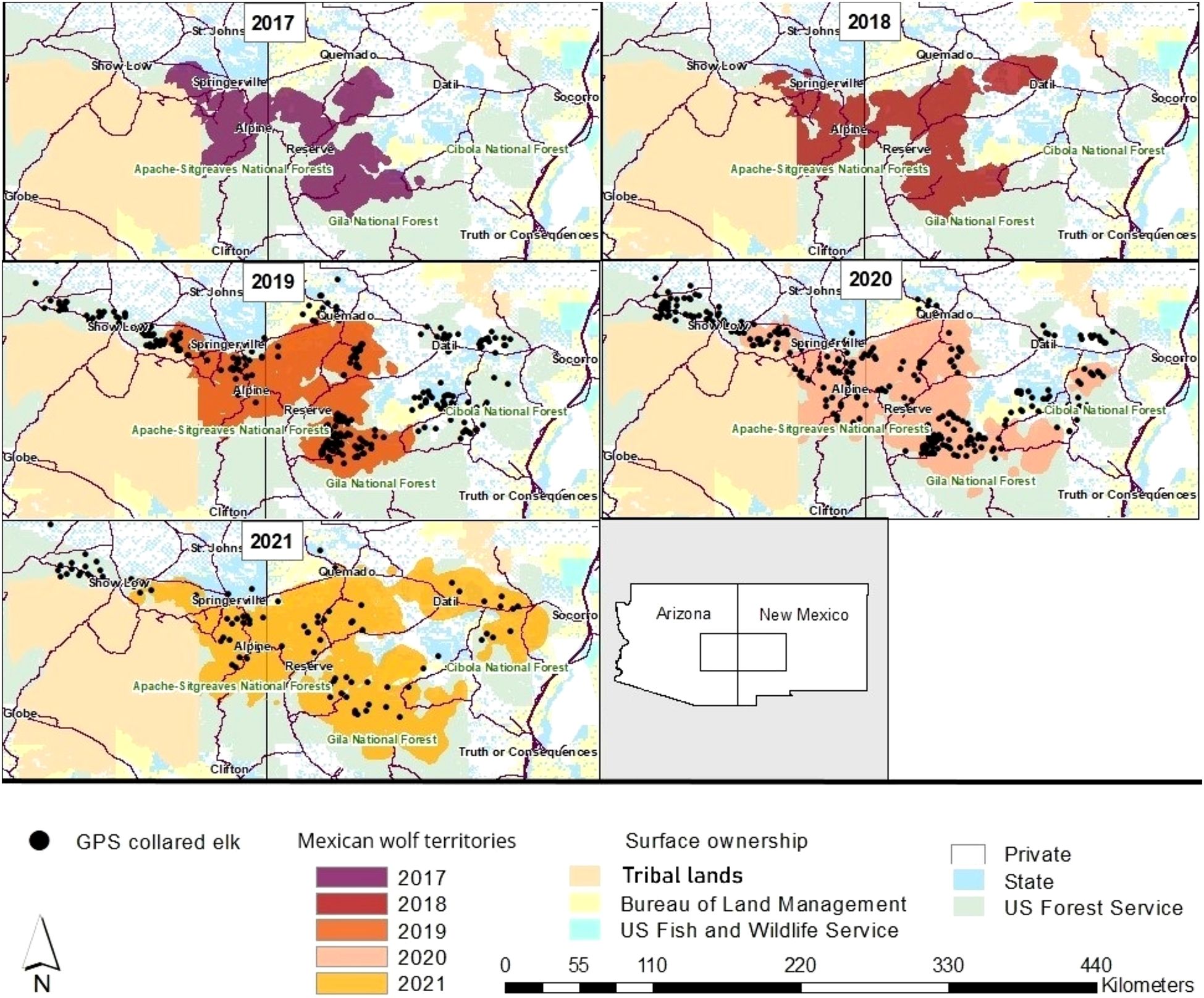
Figure 1. Map of GPS collared elk (n = 439) used in the step-selection analysis in relation to wolf territories in the Mexican wolf experimental population area. Consistently occupied territories typically indicate more established or “high” wolf density areas. Note that over the duration of this project there have been collared elk in areas that have gone from no wolves to low or moderate wolf density areas. An agreement between local tribes and USFWS restricts depictions of wolf data on tribal lands, thus wolf use and elk locations in these regions are excluded from figures. Each elk point reflects one randomly selected GPS location per individual for each respective year. Data in 2021 represent January to June.

Dominant vegetation communities at higher elevations are primarily spruce-fir and mixed conifer forests which include Engelmann spruce (Picea engelmannii), sub-alpine fir (Abies lasiocarpa), Douglas‐fir (Pseudotsuga menziesii), white fir (Abies concolor), and aspen (Populus tremuloides). Ponderosa pine (Pinus ponderosa) and Gambel oak (Quercus gambelii) compose mid-elevation vegetation communities and low elevation areas primarily consist of alligator juniper (Juniperus deppeana), oneseed juniper (J. monosperma), and piñon pine (Pinus edulis). Cool and warm season grasses are interspersed throughout and produce large swaths of high elevation montane grasslands and low elevation plains. Forest fires are common, with large (> 297,844 acre) stand replacing fires occurring in 2011 and 2012. Aside from elk, native ungulates include mule deer (Odocoileus hemionus), Coues white-tailed deer (Odocoileus virginianus couesi), pronghorn (Antilocapra americana), javelina (Pecari tajacu), and Rocky Mountain bighorn sheep (Ovis canadensis canadensis). Predators in addition to Mexican wolves include mountain lion (Puma concolor), black bear (Ursus americanus), coyote (Canis latrans), and bobcat (Lynx rufus).

Climate is generally mild with warm summers and moderate to cold winters. Average annual precipitation is 68.7 ± 12.1 cm (SD) for high elevation areas (≥ 2,684 m) and 36.7 ± 6.7 cm (SD) for low elevation areas (≤ 1,975 m), with snowfall averaging 193.2 ± 105.3 cm (SD) and 44 ± 43.4 cm (SD) in high and low elevations, respectively (30-year normals; PRISM Climate Group, 2021, Western Regional Climate Center, 2019). Approximately half of precipitation falls during monsoon season (June through September). Mean daily high/low temperatures for high elevation areas are 22.5°C/7.7°C in summer and 5.2°C/−7.7°C in winter (PRISM Climate Group, 2021). Mean daily high and low temperatures for lower elevation areas are 30.2°C/11.9°C and 10.6°C/−6.2°C for summer and winter respectively (PRISM Climate Group, 2021).

Methods

Study animal capture

Between January 2019 and April 2021, we captured 866 adult female elk using net-guns from helicopters, ground darting, clover traps, and corral traps. Captures primarily occurred between January and early April each year. All captured elk were fitted with GPS-Iridium collars (Advanced Telemetry Systems, model G5-2D Iridium, Isanti, MN). Collars were initially set to a 2-hour GPS fix interval but in July 2020 were changed to a 4-hour fix interval to conserve battery. Approximately half (47%) of the captures were in areas with high wolf densities while the other half (53%) occurred in areas with low wolf densities or regions without established packs (Figure 1). All capture and handling procedures were approved by New Mexico State University Institutional Animal Care and Use Committee (IACUC permit #2021-012).

The Mexican Wolf Interagency Field Team annually captured and fitted Mexican wolves with GPS collars using helicopters and foothold traps as part of their routine monitoring efforts. Helicopter captures typically occurred in January−February and foothold trapping took place late summer through fall. Collars were typically set to a 13-hour GPS fix interval, but occasionally collars were set to 6-hour, 2-hour, or 1-hour intervals depending on the age and make of the collar and specific management or research goals. Approximately 60% of Mexican wolves were fitted with GPS collars and nearly all known packs contained at least one functioning GPS-Iridium collar for the duration of this study.

Temporal partitions

We identified ecologically relevant seasons and daily activity periods for elk (Roberts et al., 2017; Kohl et al., 2018). We grouped months with similar average temperature and precipitation using PRISM 30-year averaged climate data with respect to seasonal variation in elk body condition, available nutrition, and external pressures such as hunting. The resulting seasons were winter (Dec.–Mar.), spring (Apr.–Jun.), monsoon (Jul.–Sept.), and fall (Oct.–Nov.). Following Ensing et al. (2014) and Kohl et al. (2018), we used locomotion as an index of elk activity to delineate diel periods in which behavior would be similar. For each season, we calculated movement rate (km/2 hrs) and defined diel periods in relation to civil twilight (winter n = 661,915 locations [662 elk]; spring n = 940,938 [743 elk]; monsoon n = 455,867 [527 elk]; fall n = 244,159 [374 elk]). Activity was consistently bimodal across seasons where the first peak in movement (i.e., dawn) began approximately an hour before morning civil twilight and lasted two hours after, and the second peak in activity (i.e., dusk) began approximately two hours prior to evening civil twilight and lasted for an hour after (Figure 2). We classified periods of low activity following each peak as midday (reference category) and night.

Figure 2

Line graphs display movement rates of elk and wolves across four seasons: winter, spring, monsoon, and fall. The elk's movement, indicated by a blue line, peaks during civil twilight hours, marked by shaded areas. The wolf's movement, shown by a green dashed line, remains higher throughout the day. X-axis represents time of day; y-axis shows movement rate in kilometers per hour.

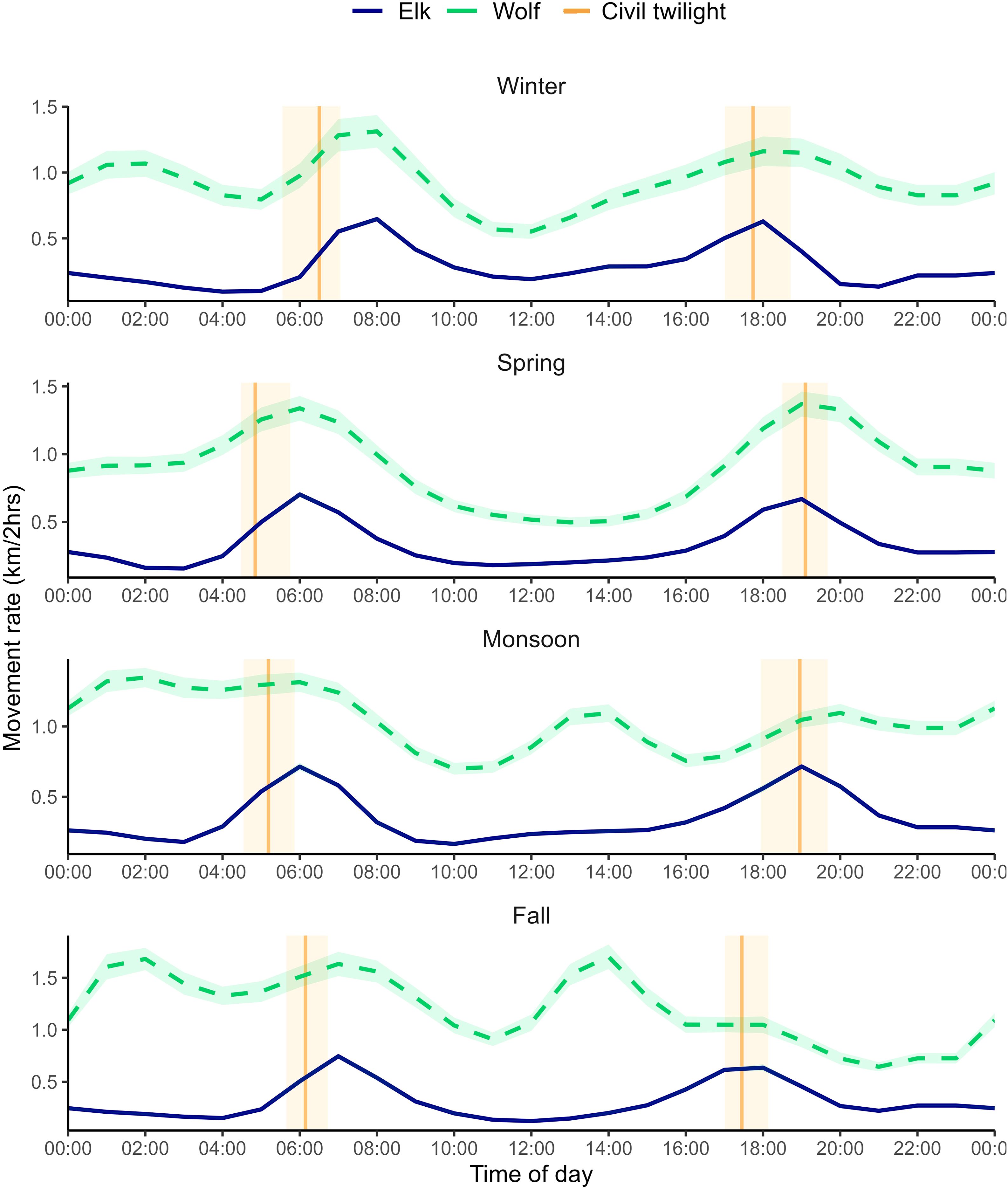
Figure 2. Activity rate (km/2 hrs) of Mexican wolves from 2017–2021 and elk from 2019–2021 in the Mexican wolf experimental population area for each season with 95% confidence bands. Vertical bands indicate seasonal civil twilight with the darker vertical line depicting the average (UTC −7). The confidence bands around elk activity are narrow, but present.

Landscape covariates

Using LANDFIRE data on vegetation communities (2016) and ArcGIS (version 10.6, Esri, 2017), we condensed existing vegetation types into eight categories to reflect dominant vegetation communities in the study area: oak/shrubland, aspen, piñon-juniper, ponderosa, grassland, mixed conifer, wet meadow/pasture and other. We then created an ecotone layer depicting where forested vegetation types met with open vegetation types to calculate distance to ecotone. We derived fire age, burn perimeters, and burn severity from the National Interagency Fire Center (NIFC, 2021) and Monitoring Trends in Burn Severity (MTBS Project, 2019) data repositories and condensed burn severity categories into unburned, low severity, moderate severity, and high severity, integrating the increased greenness category with low severity burns and the masked category with unburned. Following Crabb et al. (2022), we converted the reclassified severities into a continuous predictor, which is appropriate for ordinal data and reduces the number of parameters estimated. Because burn severity is most meaningful in relation to fire age, we included it as a predictor interacting with fire age. We classified fire age as: 0 (unburned or > 17 years old; reference category), 1 (> 0 and ≤ 5 years old), 2 (> 5 and ≤ 13 years old), and 3 (> 13 and ≤ 17 years old). We also evaluated a binary burned variable to evaluate whether a simpler representation of fire on the landscape may be more parsimonious. To assess the influence of solar radiation, terrain, and aspect related vegetation patterns, we extracted slope, elevation, and aspect from 30 x 30 m LANDFIRE data (2016) to each location and transformed aspect into continuous northness index ranging from −1 to 1, with values closer to 1 representing north facing aspects. Peterson et al. (2021) indicated metrics of topographical complexity might capture how elk perceive risk more accurately, so we created a vector ruggedness measure (VRM) and terrain ruggedness index (TRI) using the spatialEco package in R (Evans and Murphy, 2021; R Core Team, 2021). To evaluate water, we combined U.S. Geological Survey National Hydrography Datasets with locations of anthropogenic water sources provided by the U.S. Forest Service and Bureau of Land Management and calculated distance to nearest perennial water sources for each location. To assess recreational features, we extracted minimum distance to trails, developed campgrounds and lakes, ski resorts, and high-traffic areas of Sipe White Mountain and Wenima Wildlife Areas. To quantify the effects of roads, we classified roads into three categories: paved or well-maintained dirt roads with a relatively high degree of travel (1), gravel and dirt roads which experience less travel and/or require moderate clearance (2), and unmaintained dirt roads requiring a high clearance vehicle (3). Using these reclassified road layers, we generated road density rasters at a 1.5 x 1.5 km scale. To represent forage conditions, we calculated the Normalized Difference Vegetation Index (NDVI) from 8-day and 16-day MODIS satellite imagery. We acquired daily snow depth data, representing a measure of winter severity, from the National Oceanic and Atmospheric Administration’s National Operational Hydrologic Remote Sensing Center Snow Data Assimilation System. To assess how visual obstruction influenced elk habitat selection, we extracted percent canopy cover from the National Land Cover Database (Multi-Resolution Land Characteristics Consortium, 2016) and developed an index of horizontal cover derived from LANDFIRE existing vegetation cover and height layers (2016). We reclassified vegetation height to reflect an elk’s potential to visually detect a predator; 0- indicating vegetation < 1 m tall (open), 1- indicating vegetation 1–2 m high (tall enough to potentially hide a wolf or lion), and 2- indicating vegetation ≥ 2 m in height (full visual obstruction to an elk). Then, we reclassified vegetation cover in context to dominant structure where open areas (0) were locations with woody vegetation cover < 30% and closed-canopy areas (1) were areas with ≥30% woody cover. We multiplied the two reclassified metrics together to create the horizontal cover covariate.

Spatial risk covariates

In addition to landscape covariates, we created three metrics representing spatial variation in wolf predation risk because it is unclear how elk perceive spatial risk (Moll et al., 2017). Risk metrics included openness, predicted wolf presence, and a “risky places” index derived from landscape attributes of wolf-killed elk.

Openness

Elk appeared to associate openness with perceived wolf predation risk in the Greater Yellowstone Ecosystem (Creel et al., 2005; Mao et al., 2005; Kohl et al., 2018). Therefore, we created indices of openness at two spatial scales, where the number of open pixels (< 30% canopy cover) were summed around a focal pixel centered within a 250 x 250 m or 500 x 500 m moving window (Boyce et al., 2003; Kauffman et al., 2007).

Predicted wolf presence

Because the Mexican wolf population has been expanding in size and distribution on the landscape, we calculated multiple measures of wolf presence as proxies for predation risk. These risk indices are products of a wolf habitat selection function (HSF) and various wolf utilization distributions (hereafter referred to as UDs; Hebblewhite and Merrill, 2007). To create seasonal wolf HSFs, we tested 40–45 a priori models (Supplementary Table S2) for each season using a 1:10 used:available ratio of 129,925 spatiotemporally independent GPS locations collected from 137 wolves from January 2017 through June 2021 (See Supplementary Material: Predicted wolf presence index for details).

We estimated wolf UDs using kernel density estimators in the R package adehabitatHR (Calenge, 2006; R Core Team, 2021). We created population-level and pack-level UDs for each year (_Y) and seasonally within each year (_SY) from December 2018 through June 2021. To assess whether the presence of wolves, regardless of how many, affects elk habitat selection we used population-level UDs of one wolf per pack, pooled across packs, representing the general occupancy of wolves within the study area. To create pack-level UDs, we utilized all spatiotemporally independent locations within a pack and multiplied each UD by its corresponding pack size per temporal scale (max [_m] and average[_a]), then merged the pack UDs, adding values that overlapped in space (See Supplementary Material: Predicted wolf presence index for details). Prior to multiplying the HSFs and UD values together, we added 1 to the HSF values and 2 to the UD values. This prevents an area with no wolves (UD value = 0) canceling out the value of the HSF (and vice-versa) and places more weight on actual use rather than predicted use based only on the HSF. Multiplying the values accounts for landscape attributes that elk may evolutionarily associate with wolf presence, weighted by actual relative intensity of wolf use.

Risky places

Because kill sites represent the endpoint of an accumulation of predation risk, we compared site characteristics from confirmed wolf-killed elk to random locations within respective wolf territories using mixed-effects logistic regression with a random intercept for wolf pack (Kauffman et al., 2007). Mortalities included collared elk and carcasses discovered during wolf cluster investigations, however, we only analyzed female elk and elk calf mortalities (n = 306) because male ungulates utilize the landscape differently (Christianson and Creel, 2008; see Supplementary Material: Risky places index for details). Parameter estimates derived from the most-supported model reveal landscape characteristics that likely contribute to kill success, which elk may perceive as risky.

Temporal variation in predation risk

To represent temporal variation in wolf predation risk, we used wolf diel activity because movement rate of wolves has been directly associated with encounter rates of elk and successful kills (Kohl et al., 2018). Additionally, Ensing et al. (2014) found movement to be a meaningful representation of foraging activity for large mammals. We matched the temporal interval of wolf and elk movements and seasonally calculated kilometers traveled per two hours using data from 57 spatially independent, non-dispersing wolves with GPS collars programmed to 1–2-hour fix rates (winter n = 9,727 [24 ind.]; spring n = 15,192 [39 ind.]; monsoon n = 11,115 [22 ind.]; fall n = 5,617 [13 ind.]; Kohl et al., 2018; Figure 2). Due to the 2-hour lag inherent in the distance calculations, we shifted movement rates back one hour. This captures the activity as occurring between the start and end times, rather than at the end time. To estimate population-level patterns of wolf activity, we fit a generalized additive mixed model using a negative binomial to address the skewed nature of the movement data (Fortin et al., 2005; Kohl et al., 2018) and included a random intercept for wolf ID to account for individual variation in movement rates. Each seasonal model utilized a cyclic cubic regression basis spline with 12 knots.

Using seasonal activity rates of wolves, we created a categorical diel period variable to account for temporal variation in wolf habitat selection. For each season, consecutive times with similar activity rates were grouped together and defined relative to seasonal average civil twilight as either morning, midday, evening or night (such as with elk in Temporal partitions). For each GPS location, civil twilight was calculated based on date and location and diel period was assigned based on the time of the fix relative to that day’s civil twilight and the season.

Analysis of elk habitat selection

We resampled elk locations to 4-hour fix intervals and truncated locations from seven days post-capture through one day prior to mortality. Following Fortin et al. (2005), we paired each GPS location, or “step”, with ten random alternative points (originating from the same starting location) drawn from individual-specific distributions of turn angles and step lengths using the amt package in R (Signer et al., 2019). To reduce spatiotemporal autocorrelation, we thinned steps where locations of multiple elk were ≤ 500 m from each other at the same date/time and for each individual, where used locations were ≤ 100 m from each other within a 24-hour period. At 4-hour fixes, the truncated and thinned data amounted to over 2 million used locations, so to improve computational speed, we reduced the used data to a random 75% of locations for each animal and required individuals to have data for > 65% of a season and > 50% of a year. We extracted landscape covariates and calculated estimated predation risk for observed and alternative (available) locations in R. Prior to model building, we centered and scaled predictor variables by season and tested for multi-collinearity using Spearman’s correlation coefficient for pairs of continuous and/or ordinal variables and chi-squared tests for categorical variables, in addition to assessing if variables had near-zero variance. Predictors with a Spearman’s correlation coefficient (|ρ|) ≥ 0.7 or with near-zero variance were not included together in model building. Elevation was highly correlated with predicted wolf presence and dominant vegetation was highly correlated with risky places and thus were excluded from the analysis. Due to collinearity between openness at the 500 m scale and canopy cover, only openness at the 250 m scale was evaluated. Preliminary modeling revealed parameter estimates stabilized at a 1:5 used:available ratio (Fieberg et al., 2021; Supplementary Figure S8), so we randomly selected 5 alternative locations per used step, considering points in water bodies or on extreme slopes (> 60 degrees) as unavailable, then re-centered and scaled predictors.

We partitioned and modeled the data seasonally to reflect ecologically relevant scales of selection (Ensing et al., 2014; Roberts et al., 2017). Using the inhomogeneous Poisson process (IPP) methodology described in Muff et al. (2020), we estimated relative intensity of elk use via a mixed-effects step-selection function (SSF; Duchesne et al., 2010) using the glmmTMB package (Brooks et al., 2017). Models were conditional on step ID and included random slope terms for predictors and a random intercept for animal ID to account for potential functional responses (fall n = 414 ind.; spring n = 433 ind.; monsoon n = 439 ind.; winter n = 204 ind.; Gillies et al., 2006; Muff et al., 2020). Because we were interested in the role of wolf predation risk on elk habitat selection, we first tested 62 a priori base models for each season to establish elk habitat selection relative to landscape characteristics and resources (Johnson et al., 2021; Crabb et al., 2022). Model formulas were designed to explore relationships between elk and seasonal environmental elements based on peer-reviewed literature and expert knowledge. We incorporated distance to private land, recreation sites, and high-use roads to account for the influence of human presence on elk. Public land tends to have higher concentrations of hunters, which can cause ungulates to take refuge on private lands (Sergeyev et al., 2022), whereas during calving season, elk may utilize human refugia as predators tend to avoid people (Hebblewhite and Merrill, 2009). Building upon the best base model for each season, we incorporated spatial risk covariates and interactions between spatial and temporal risk to capture the dynamic nature of predation risk (Kohl et al., 2018; Johnson et al., 2021; Supplementary Material: Analysis of elk habitat selection). Spatial risk metrics included openness, predicted wolf presence (wolf HSF*wolf UD), intensity of wolf use (UDs), risky places, risky places relative to wolf use, interactions between openness and predicted wolf presence, and openness relative to wolf use. For temporal risk, we evaluated interactions between spatial risk with both elk diel period and wolf activity. We selected the best models for each season using AIC. We validated the most-supported models using 50 repeats of a 10-fold cross-validation appropriate for mixed models (Spearman’s rho [ρ]) and assessed used-habitat calibration plots (Fieberg et al., 2018) as they may be more appropriate than k-fold techniques, given the conditional nature of SSFs. We also verified independence between predictors by ensuring variance inflation factor (VIF) scores were < 2.5.

Following Avgar et al. (2017), we calculated the relative selection strength (RSS) of predation risk by using the most-supported model for each risk index. This method quantifies the average change in probability of space use as predation risk changes, while all other covariates are at their mean/reference value. We log-transformed RSS so negative values indicate avoidance and positive values indicate selection (Avgar et al., 2017; Crabb et al., 2022). Using the most-supported wolf use x temporal risk model for each season we investigated how use of landscape terms was affected by changes in spatiotemporal risk. This analysis utilized wolf UDs to avoid potential circularity between risk metrics derived from landscape covariates (e.g., predicted wolf presence and risky places) and base elk SSF terms. For all interaction terms evaluated, relative intensity of use was compared to the estimated use of the standardized average value (0) of the landscape term at the smallest UD value. We examined how spatiotemporal predation risk affects selection of TRI (Mao et al., 2005), burn, canopy cover (Fortin et al., 2005), distance to ecotone, and distance to roads by elk because these relate to forage opportunity and quality, but are also relating to hunting and space use by wolves (Hebblewhite et al., 2005; Dickie et al., 2017).

To investigate if habitat selection changes in relation to the intensity of wolf use, for each elk we extracted wolf use values for GPS locations during the initial season-year the elk was captured, then calculated the median wolf UD value to assign one of four risk levels. We designated risk categories based on where the median value fell in relation to the quartile distribution for the Pack_Ym UD (Supplementary Material: Analysis of elk habitat selection). Elk in the first quartile were considered naïve or minimally exposed to wolves, with no known established wolf territories occurring in these areas (denoted as “no known” in initial risk strata). Elk with low initial risk typically occurred in the periphery of occupied wolf territories or in newly established wolf territories with a small number of individuals, whereas elk with high initial risk primarily spent their time in the core area of a larger pack or in locations frequented by multiple packs; elk with moderate initial risk lay in-between criteria. We partitioned the data by season and initial UD quartile and evaluated the top spatiotemporal risk models using AIC. For each of these models, we then calculated the log-RSS to depict the magnitude of the effect a spectrum of risk has on elk habitat selection and evaluated how exposure to risk might influence use.

Results

Spatial risk proxies

Predicted wolf presence

Relative selection for environmental variables was similar across seasons except for fire age and distance from trails and recreation areas (Supplementary Figure S4). Models including interaction terms with diel period did not perform better than those without the interaction (Supplementary Table S4). Cross-validation indicated high model predictive accuracy for all seasons (ρ ≥ 0.99). Wolves selected areas closer to water, moderate elevations, farther from private land, and closer to unmaintained, high clearance roads, trails, and recreation areas. Wolves strongly selected for burns ≤ 5 years old and avoided intermediate aged burns throughout the year compared to unburned areas. During spring and monsoon, wolves moderately selected older burn scars, but avoided such burns in fall and winter (Supplementary Figure S4).

Risky places

The top performing model describing wolf-killed elk sites included dominant vegetation type, openness at the 500 m scale, slope, northness, distance to all roads, distance to recreation areas, and whether the area had been burned in the past 17 years (Supplementary Figure S5). The Spearman’s ρ value in 10-fold cross validation was 0.99. Dominant vegetation was the most influential predictor, followed by distance to trails/recreation sites, distance to all roads, burn, slope, and openness. Kills were more likely to occur in aspen and wet meadow/pasture than grassland and less likely to occur in piñon-juniper and ponderosa compared to grassland. The likelihood of kills occurring in mixed conifer and oak shrubland did not differ from grassland. Areas that were riskier included those closer to roads and recreation sites, burn scars, more open areas, intermediate slopes, and south-facing aspects.

Temporal risk

Seasonal wolf activity patterns were variable, but generally were highest at dawn, followed by the middle of the night (except in spring), dusk, early night (shortly after dark), then midday (except for fall and monsoon; Figure 2). Spring wolf activity exhibited a bimodal pattern where movement rates associated with hunting were greatest at dawn and dusk, followed by moderate movement at night, and low activity at midday. Winter activity patterns were similar to spring, however, there was less of a midday lull in activity and movement after midnight increased to create a third peak in activity (Figure 2). A “trimodal” pattern is also seen in monsoon season, where movement rates are highest at night through morning—followed by smaller peaks in activity mid-afternoon and evening. In fall, activity peaks after midnight, at dawn, and mid-afternoon, with movement lowest after sundown. Activity patterns were relatively variable across years except in spring (Supplementary Figure S15).

Elk habitat selection

Base models

The most-supported landscape models for fall, spring, and monsoon season included fixed effects for canopy cover, distance to ecotone, distance to all roads, TRI, a quadratic term for 16-day NDVI, northness, burn, interaction terms between diel period and canopy cover, distance to ecotone, and distance to all roads (Supplementary Table S9). The best winter model was similar to other seasons but excluded NDVI and northness and instead contained quadratic terms for distance to water and TRI. Elk selected for intermediate vegetation greenness and more north-facing slopes spring through fall, while in winter they selected for moderate distances to water. Adult female elk selected for low to moderate terrain ruggedness and burned areas, and selected for areas closer to roads, with less canopy cover, and closer to ecotones during dawn, dusk, and night, compared to midday (Supplementary Figure S9). All most-supported models had VIF scores < 2 and 10-fold cross validation indicated high predicative performance of the top seasonal models (all ρ ≥ 0.93 Supplementary Material: Analysis of elk habitat selection).

Spatial risk

Across seasons, adding a spatial risk term to the base landscape model improved performance, regardless of the risk metric used. However, the most influential spatial risk metric in elk habitat selection changed with each season (Table 1; Supplementary Material: Analysis of elk habitat selection). In all instances, the effect of risk appeared to be non-linear and models containing quadratic main effects outperformed those with only linear terms (Table 1). In fall, the most-supported spatial risk metric was predicted wolf presence, while in winter, openness was most supported (Figure 3). In spring, openness relative to predicted wolf presence was most supported and during monsoon season, risky places was the most influential index of risk (Figure 3). Overall, seasonal, population-level wolf UDs were more supported than yearly and pack-level UDs, except during winter and fall, when metrics accounting for pack size were more influential (Table 1). Additionally, there was no substantial difference between pack-level UDs which used the maximum versus mean number of individuals per year; each had nearly identical effects across seasons, typically being within ΔAIC ≤ 3 of each other. Models containing random slopes for predation risk terms consistently outperformed those without (Supplementary Material: Analysis of elk habitat selection).

Figure 3

Four-panel plot showing the relationship between risky places and log RSS across different times of day: Dawn, Midday, Dusk, and Night. Lines represent seasons: Winter (red), Spring (green), Monsoon (blue), and Fall (purple), with shading indicating confidence intervals. Dawn, Dusk, and Night show increasing trends, while Midday shows a decrease.

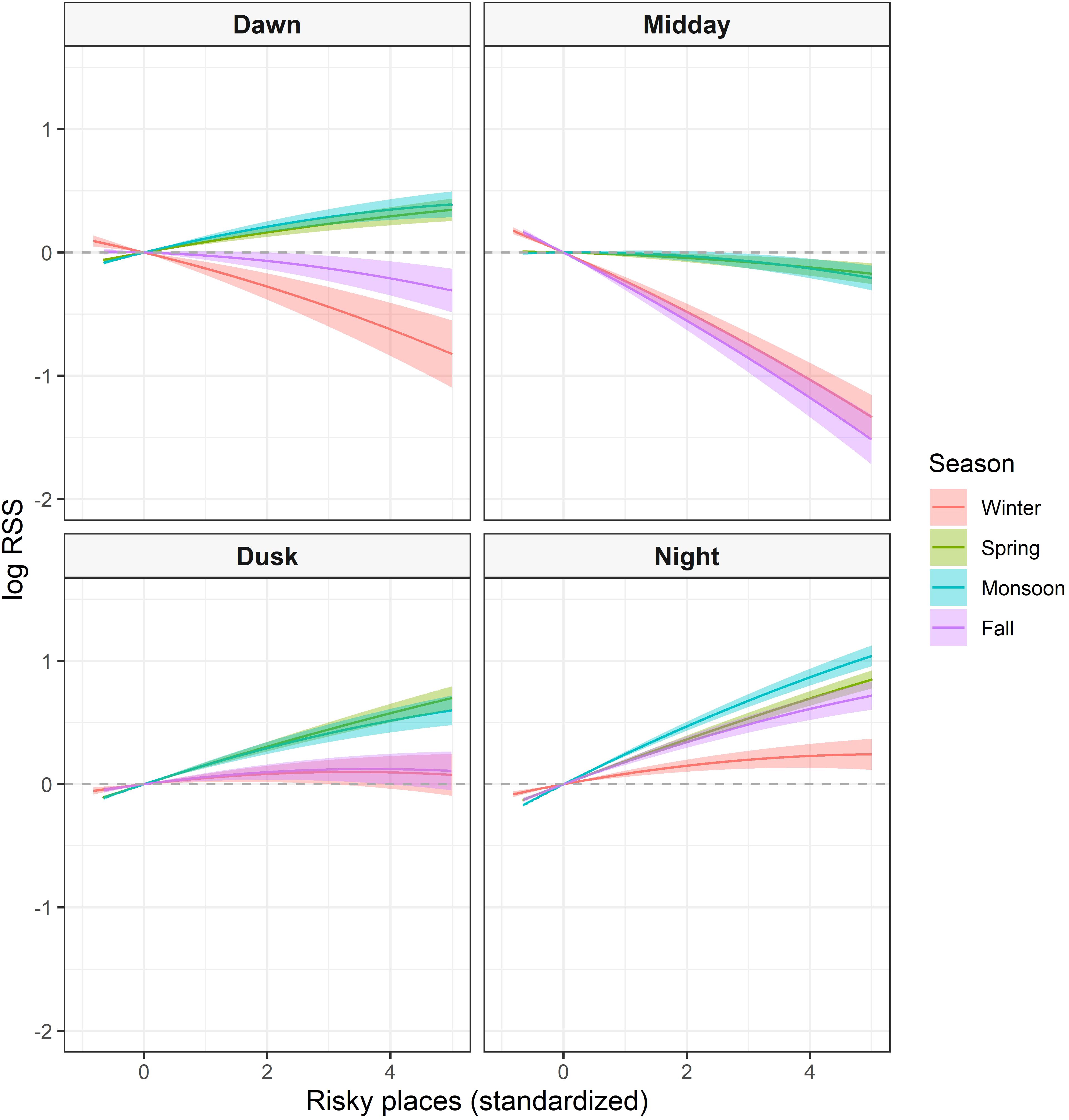
Figure 3. Seasonal log relative selection strength (RSS) with 95% confidence bands of elk within the Mexican wolf experimental population area between 2019–2021 comparing the difference in relative intensity of use between the average risk value of the landscape to all other locations. For ease of interpretation, results were truncated to display 99.8% of data.

Table 1

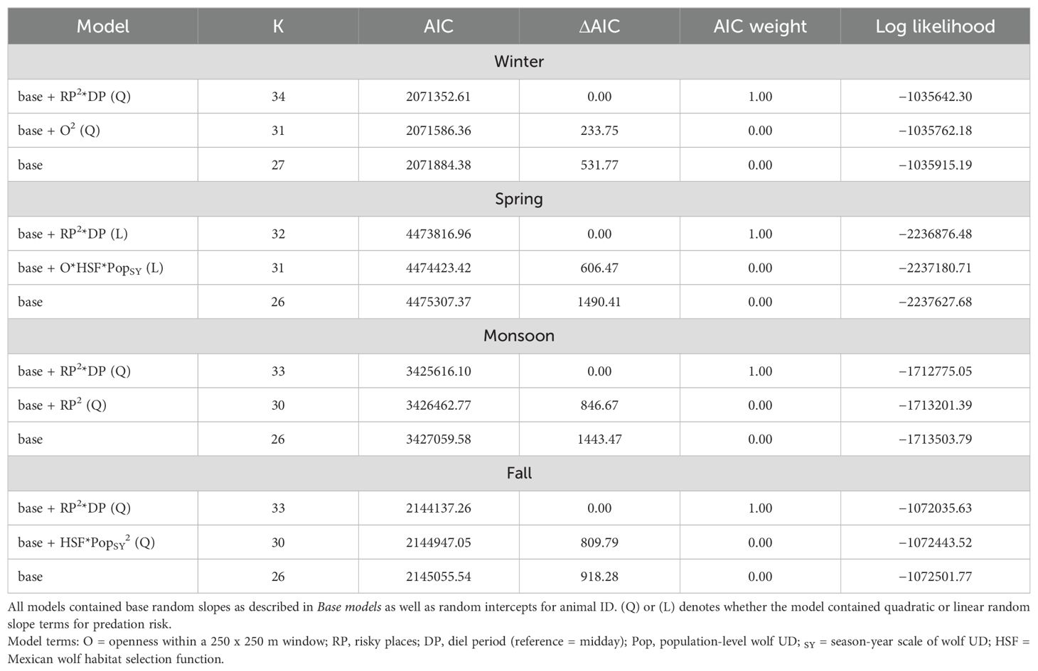
Table 1. Comparison between best base model (Supplementary Table S9), base + spatial risk model, and base + spatiotemporal risk models for each season evaluating influence of predation risk in elk habitat selection in western Arizona and eastern New Mexico, 2019–2021.

Spatiotemporal risk

Incorporating an interaction between spatial and temporal predation risk indices improved model performance (Table 1). Diel period was influential across seasons and improved all spatial risk models whereas wolf activity was not as influential (Table 1; Supplementary Table S10). Once an interaction with diel period was included, the top performing risk metric changed for winter, spring, and fall to risky places. Therefore, across seasons, risky places with respect to diel period and the base landscape variables best explained relative elk use on the landscape.

Across seasons, use of areas with higher-than-average risky places values by elk was more likely during dusk and highest during night (Figure 4). Use of risky places during dusk occurred more intensely during spring and monsoon seasons and was less intense at night and dusk during winter. In fall and winter there was a strong avoidance of riskier places midday, while in spring and monsoon seasons there was only a slight avoidance for areas associated with wolf-killed elk sites. At dawn, elk avoided riskier places most intensely during winter but also during fall, whereas in spring and monsoon seasons, elk conversely selected for riskier areas. Top performing spatiotemporal risk models had VIF scores < 2.5 and 10-fold cross validation revealed strong predicative performance of the top seasonal models (all ρ ≥ 0.99; Supplementary Material: Analysis of elk habitat selection). Used-habitat calibration plots also indicated adequate to strong model performance, across seasons, for each covariate (Supplementary Figure S11).

Figure 4

Graph grids showing the effect of initial wolf risk strata (no known, low, medium, high) at different times (dawn, midday, dusk, night) for each season (winter, spring, monsoon, fall). Each grid displays curves showing relative selection of risky places with shaded areas representing variability. The x-axis represents standardized risky places, while the y-axis depicts log relative selection strength on a negative to positive scale, with negative numbers representing avoidance and positive numbers indicating selection.

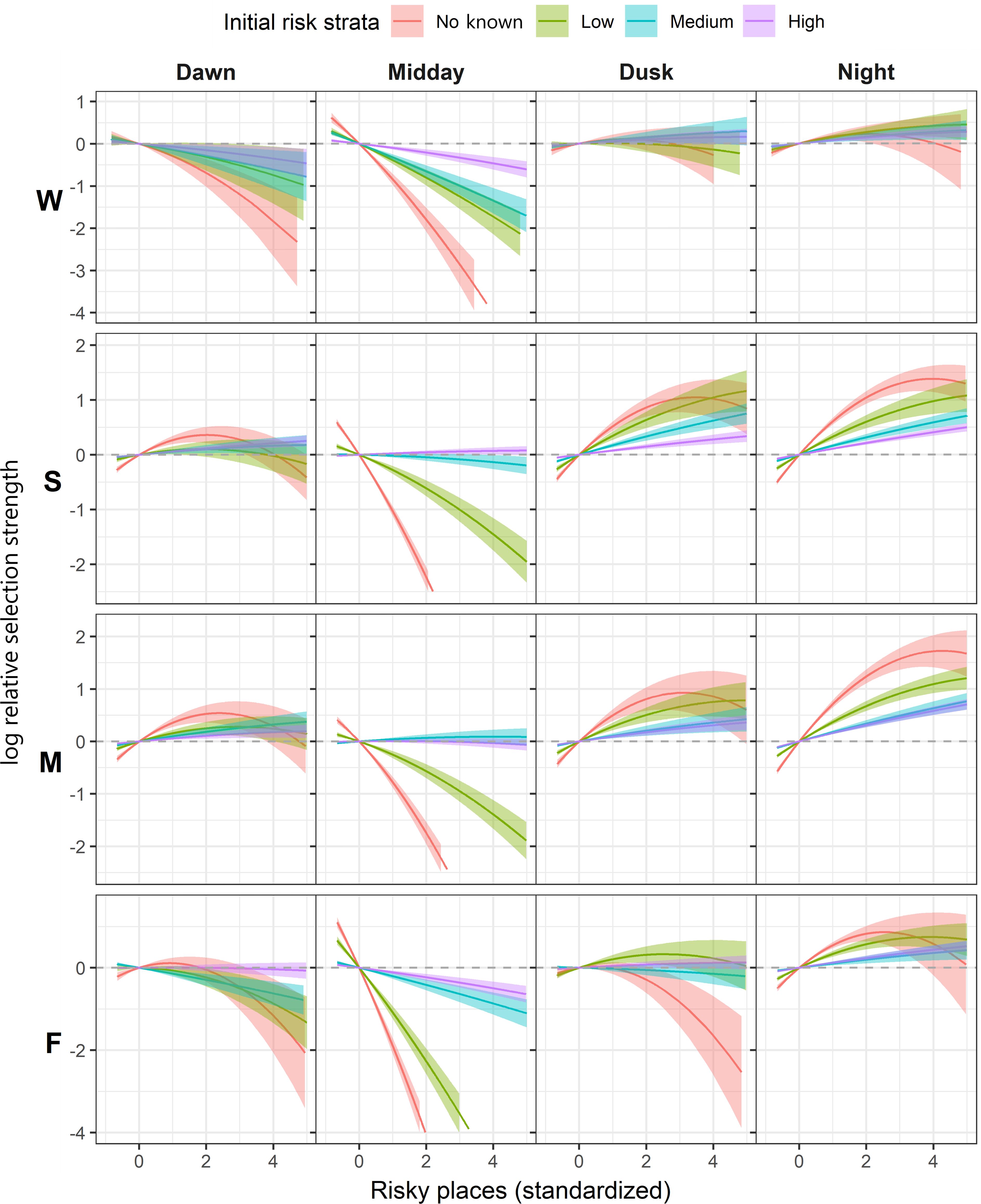
Figure 4. Seasonal log relative selection strength (RSS) with 95% confidence bands of elk within the Mexican wolf experimental population area between 2019–2021 comparing the difference in relative intensity of use between the average risk value of the landscape to all other values in relation to intensity of wolf presence at time of capture. W, winter; S, spring; M, monsoon; F, fall. For ease of interpretation, results were truncated to display 99.8% of data.

The post-hoc analysis evaluating the top performing wolf use x temporal metric interacting with base landscape covariates revealed use of canopy cover by elk was most affected by wolf use, while distance to ecotone and use of burned areas were not dependent upon how intensely wolves used those features (Supplementary Material: Analysis of elk habitat selection). In areas with no to low wolf use elk were significantly more likely to use open areas at dusk for all seasons and forested areas during midday, but as intensity of wolf use increased, differences in relative use by elk of different canopy cover levels diminished at these times for all seasons but fall (Supplementary Figure S12). A loss of distinct use patterns between different levels of terrain ruggedness and distance to roads also occurred as wolf use increased, but to a lesser degree (Supplementary Figures S13, S14). Additionally, elk were consistently more likely to use open canopy at night than closed canopy in all seasons but winter, regardless of wolf use (Supplementary Figure S12). In all cases, the interaction model outperformed the additive spatiotemporal model.

Risk strata and habitat use

Partitioning the collared elk by their initial risk strata revealed a functional response, indicating use of risky places by elk changes relative to the amount of risk encountered within their home ranges. For elk with moderate to high initial risk strata use in relation to risky places was more conservative (whether selecting or avoiding), compared to more naïve elk with low wolf exposure. More naïve individuals often exhibited the most dramatic response to risky places, particularly in spring and monsoon seasons. When compared to the relative intensity of use of the average risky places value on the landscape, elk residing in areas where wolves were least likely to be encountered strongly avoided areas with high risky places values midday, followed by elk with low wolf exposure (Figure 4). Elk with moderate or high initial exposure to wolves also avoided riskier areas midday in fall and winter, but to a much lesser extent; during spring and monsoon their relative use of risky places midday was significantly more intense than individuals with less wolf exposure (Figure 4). Across seasons and diel periods, the relative intensity of use of riskier areas declined in naïve elk and to a lesser degree, elk with lower wolf exposure. Interestingly, across risk strata and seasons, elk selected for riskier places at night, despite relatively high levels of wolf activity during most seasons and more wolf kills occurring at night (49%) than any other diel period.

Discussion

Adult female elk within the MWEPA employed spatiotemporal avoidance strategies at both a seasonal and diel scale to mitigate predation risk from Mexican wolves. Elk also showed a functional response, suggesting the way elk used risky places depended on their level of exposure to wolves. Our results are consistent with research emphasizing the importance of accounting for temporal variation in predation risk (Lima and Bednekoff, 1999; Creel et al., 2008; Kohl et al., 2018, 2019, Smith et al., 2019), but also reveal the hierarchal nature of changes in elk habitat selection over time by examining variation in spatiotemporal avoidance strategies in different seasons in relation to wolf presence. Once a temporal component is incorporated into habitat selection models including spatial risk metrics, it becomes evident that risk avoidance also occurs at a finer scale in space and time that corresponds with activity budgets and dynamic behavior of both predator and prey (Lima and Bednekoff, 1999; Middleton et al., 2013b; Kohl et al., 2019).

The type of risk which was most influential changed with the inclusion of an interaction with diel period and the risk term, resulting in risky places being the most-supported risk metric across all seasons. Within every season, all top spatiotemporal models contained either a risky places or openness metric. These spatial risk indices are the most predictable predation risk cues for elk as they are relatively static in space. Metrics like relative intensity of wolf use and predicted wolf presence may have been less supported because they represent a coarser temporal scale of risk and wolf use on the landscape is much more dynamic than landscape characteristics, thus less predictable. Predicted risky places are associated with more direct consequences for adult female elk, representing the capture component of predation risk (Hebblewhite et al., 2005), and thus it is most beneficial for elk to mitigate the component of risk which affects fitness the most (Lima and Dill, 1990; Lima and Bednekoff, 1999). Conversely, all other metrics represent various forms of encounter risk, which is a component of predation, but is not necessarily correlated with kill success (Hebblewhite et al., 2005; Kauffman et al., 2007; Moll et al., 2017). While the predicted risky places metric does not capture the nuances and compounding elements involved in predation (e.g., the age and health of predator and prey and the landscape features encountered during pursuit), habitat features significantly influence the outcome (Hebblewhite et al., 2005; Kauffman et al., 2007). Habitat characteristics associated with a higher probability of being killed also tended to be associated with higher availability and better forage quality for elk: pasture/wet meadows and more open areas, aspen stands, burns, and areas closer to roads, where diversity of plants may have often been higher due to seeds dispersed from vehicles and presence of ditches which concentrate water (Creel et al., 2005; Fortin et al., 2005; Spitz et al., 2018). Thus, impediments to escape and early predator detection, such as downed woody debris and thick regenerating vegetation, may make elk vulnerable to predation once encountered by wolves. This was supported by the significant role of fire scars and aspen stands in areas where elk were killed and has been demonstrated in other studies (Hebblewhite et al., 2005; Halofsky and Ripple, 2008). Additionally, in an exploratory analysis of risky places, the top performing model included a term for mean distance to fence, where it was the second most influential variable among predictors, however geospatial fence data were not available for tribal lands within the study area, so models containing this variable were removed from consideration as predictions of risky places needed to be made on tribal lands as well (Supplementary Material: Risky places index). Although distance to fence was purely an exploratory element in this analysis, it appears to be an important factor in risk, particularly to neonates, and should be considered in future studies if possible. Because wolves primarily occurred at moderate to high elevations during this study, kill site characteristics reflected this influence. Kill site characteristics may vary as wolves expand to lower elevations areas with different vegetation and habitat structure.

When individuals are nutritionally deficient, anti-predator strategies may not be implemented as intensely (Winnie and Creel, 2007, Oates et al., 2019). Our results supported this as adult female elk increased use of risky places at risky times during spring and monsoon seasons, particularly during diel periods associated with foraging (dawn and dusk) and midday. This contrasts to winter and fall behavior where elk only slightly selected and even avoided risky areas at dawn and dusk. Adult female elk may be more vulnerable in spring, and to a lesser degree during monsoon, because the nutritional demands required for late gestation and lactation are high and elk are recovering from winter months with low forage quality (Parker et al., 2009; Huggler et al., 2022). Average digestible protein and energy within this region appear to increase the most in May following snowmelt, but herbaceous biomass is generally low at this time (J. Cain, NMCFWRU, unpublished data), thus most nutritional forage does not become widely available until late June when monsoons begin, particularly during years with low winter snowfall. Average annual precipitation between 2019 and 2021 was 92% lower than the 30-year average (PRISM Climate Group, 2021) and may have exacerbated energetic and nutritional constraints of female elk and influenced the results herein. Because of the nutritional benefits that riskier places might afford, especially during spring and monsoon, female elk appear to be more willing to take chances and make trade-offs during the seasons they can best increase nutritional condition, which can influence fitness. Additionally, wolf activity is lowest during midday and is more predictable in spring due to denning, providing support for both the risky times hypothesis and risk allocation hypothesis, where female elk are likely balancing fitness costs and benefits by exploiting riskier places at less risky times (Lima and Dill, 1990; Lima and Bednekoff, 1999; Creel et al., 2008; Kohl et al., 2018). Furthermore, a concurrent behavioral study observed that during spring and monsoon the probability that an adult female elk would be foraging midday increased as predation risk increased, further supporting our findings (Farley et al., 2024). Moreover, the similar response across risk strata in winter and more pronounced differences in elk response between strata in spring and monsoon provide further evidence of the link between risky places and forage conditions because in winter there is less nutritional benefit in exploiting risky places.

The risk strata analysis revealed a functional response, where the intensity of use of risky places gradually changed as initial wolf exposure of elk increased. Elk with the least amount of wolf exposure used riskier places more intensely at dawn, dusk, and night during spring and monsoon and strongly avoided riskier places midday. In contrast, elk initially exposed to moderate to high wolf presence selected for riskier areas less intensely at dawn, dusk, and night in spring and monsoon and more intensely during midday than other seasons. These results suggest that elk may become more cautious to perceived risky places with prolonged exposure to established wolf presence and support the risk allocation hypothesis (Lima and Bednekoff, 1999). Additionally, a learning curve appears to occur, where the typically more intense selection of risky places by naïve elk decreases at very risky places. Further, this functional response to predation risk has also been observed in mule deer (Huggler et al., 2022). During our study, at dawn and dusk, elk sought areas with good foraging conditions, which typically exhibit characteristics that facilitate success of cursorial predators (Creel et al., 2005; Hebblewhite et al., 2005; Preisser et al., 2007). Additionally, wolf activity was also consistently higher at dawn and dusk. Thus, elk occupying areas with higher wolf presence may have more limited options for selecting perceived safe areas with preferred foraging conditions. This limitation may cause elk to use preferred foraging areas less during times wolves are most active to spatiotemporally mitigate predation. Elk with moderate to high initial wolf-exposure may balance increased predation costs with potential nutritional benefits that may correspond with risky places during spring and monsoon by shifting use of riskier areas during less risky times. Elk with little exposure to wolves likely do not need to temporally shift behavior patterns in order to balance wolf encounters and nutritional intake, thus select for risky places associated with foraging opportunities more intensely at dawn and dusk and prioritize thermal refuge and resting midday, supported by intense avoidance of risky places midday and more midday resting behavior than elk in moderate to high wolf risk areas (Farley et al., 2024).

In all instances, incorporating diel period improved spatial risk models and, in most instances, had more support than models with wolf activity as the temporal component, revealing mixed evidence of elk utilizing areas proportional to perceived risk and wolf activity (Kohl et al., 2018, 2019). The inconsistent response to wolf activity could be due to variability in daily wolf activity patterns across seasons within the MWEPA (French et al., 2022). Activity patterns were relatively variable across years except in spring, likely due to fluctuations in sample size, weather conditions, and human influence (e.g., hazing, recreationists, and livestock operations). Thus, we examined diel period as an alternative representation of temporal risk which is broadly representative of wolf activity but is less variable and related to specific environmental cues like sun angle and ambient temperature. Elk habitat selection in relation to predation risk was likely more responsive to diel period because it is more predictable than anticipating the variable movements of a highly mobile and wide-ranging predator and is more directly related to the behavioral state of elk. Response to predation risk should, at least in part, be related to the primary behavioral state across the diel period. For example, during foraging periods, elk may have to accept higher levels of risk to access forage than they would during diel periods when they are typically resting.

On a finer spatial scale, interaction effects between wolf use and base model terms revealed how areas with more wolf use affected the influence of other landscape characteristics on relative intensity of elk use. However, due to intensity of wolf use representing a temporally broad metric of encounter likelihood, results examining how elk respond to landscape elements differently in relation to wolf use should be interpreted with caution, as cursorial predators often overlap heavily in space with prey (Schmitz et al., 2017) and encounter metrics only represent one component necessary for predation (search–encounter–kill; Lima, 1992; Hebblewhite et al., 2005). Relative intensity of use between intermediate canopy cover often did not differ from closed or open canopy cover, which may have reflected the effects of reclassifying a continuous variable into a discrete one for visualization purposes. However, as wolf use increased, the degree of overlap between all canopy cover levels, and to a lesser degree terrain ruggedness and road use, increased. This supports the idea that seasonal predator use is too broad of a predation risk metric for species that heavily overlap in space and time and suggests elk may respond to increased encounter likelihood by shifting selection reactively, at a finer and more immediate scale, thus causing an averaging effect in selection for specific levels of landscape elements over a season (Creel et al., 2005; Middleton et al., 2013b; Basille et al., 2015). For example, open canopy is associated with increased wolf encounters, but it also provides greater nutritional benefits for elk and is easier to detect wolves in. It is unlikely elk are pursued by wolves every time they forage in open spaces, so instead of avoiding these areas, elk continue to use open spaces and rather react once wolves are detected, which may include fleeing into cover or staying in cover for a few hours longer. The variable use of open spaces dependent on wolf presence would show up as overlapping use of canopy cover types over the course of a season. The control of risk hypothesis (Creel, 2018) suggests anti-predator responses are either proactive or reactive depending on the prey’s ability to perceive, predict, and control risk. Wolves typically travel farther than elk, therefore, wolves may not frequent the same areas as often or encounter the same elk herd/individuals for several days and thus may not be perceived by elk as a persistent threat needing severe mitigation, particularly within the MWEPA as diel patterns in wolf activity are less predictable for some seasons (Schmitz et al., 2004; Preisser et al., 2007; Middleton et al., 2013b). Further research is needed to evaluate spatiotemporally fine-scale wolf–elk interactions and whether potential shifts in selection are significant enough to cause population-level non-consumptive effects.

Across all seasons, elk used riskier places at night, which may have been a product of balancing risk mitigation strategies for two predators with opposite hunting modes. Elk are the primary prey for not only Mexican wolves in the study area, but also for mountain lions (Martinez, 2024). Wolf kill sites within the MWEPA were generally associated with more open areas, consistent with Kohl et al. (2019), which found female elk utilized areas with a higher spatial likelihood of wolf predation (open areas) at night when wolves were less active to avoid mountain lions in forested areas. At night, despite moderate to high wolf activity during most seasons, elk consistently selected for open spaces over closed canopy in areas with high wolf use, except in winter when pack cohesion was greatest (Metz et al., 2011; Benson and Patterson, 2015) and the nutritional reward of open places was most limited, suggesting elk were prioritizing avoidance of mountain lions at night and potentially taking advantage of foraging opportunity. Cursorial predators may encounter elk more but have higher success in killing non-prime age individuals or those in poorer body condition (Metz et al., 2012), whereas lions may have lower encounter rates with elk, but once encountered, kill success is higher and they are less discriminate among age and condition of elk (Hornocker, 1970). Therefore, due to differences in hunting style, wolves may not be perceived by a healthy adult female elk as more lethal or risky than a mountain lion (Morosinotto et al., 2010; Kohl et al., 2019). Additionally, as ambush predators, lions are more reliant on cover and darkness for stealth, which are recognizable environmental cues predictable to prey (Hornocker, 1970; Smith et al., 2019).

Although spatiotemporal avoidance of wolves is exhibited on a seasonal and diel scale, it more proactively occurs and is strongest during seasons when the loss of associated foraging opportunities is lowest (winter, fall) and during time periods where wolf activity is more predictable (i.e., dawn). It is likely energetically inefficient for female elk to spatiotemporally avoid areas of high wolf risk completely during times of high nutritional reward due to lack of consistent spatial/temporal cues to indicate wolf presence. It does, however, seem energetically efficient for adult female elk to proactively mitigate risk from a more lethal, more spatiotemporally predictable predator with fewer nutritional costs associated with avoidance (Kohl et al., 2019). Therefore, when it comes to mitigating risk, it appears elk employ a combination of proactive and reactive responses, and shift strategies seasonally in accordance with physiological demand and reward, supporting the risk allocation hypothesis (Lima and Bednekoff, 1999). Proactive responses can have detrimental effects on nutritional condition if loss of foraging efficiency is not mitigated (Creel, 2018). Reactive responses are linked to more predator–prey encounters and thus result in learned behaviors but also can result in physiological and psychological stress such as increased glucocorticoid levels and decreased body condition (Creel, 2018). Negative effects from both strategies have the potential to affect demographic parameters like survival and pregnancy rates, thus it is necessary to consider how predation pressure, from the suite of predators elk are exposed to, can indirectly affect elk fitness in addition to consumptive effects.

Understanding non-consumptive effects requires knowledge of the mechanisms driving them (Gude et al., 2006). Thus, ongoing research is currently evaluating pregnancy rates, survival, and body condition of elk within the MWEPA to determine if non-consumptive effects are occurring because of anti-predator responses to increased wolf presence (J. Cain, NMCFWRU, unpublished data). It is important to acknowledge however, that elk co-evolved with both wolves and mountain lions and natural selection tends to favor anti-predator strategies that optimize fitness. Shifts in habitat selection and foraging behavior in areas of higher wolf presence and during times of greatest nutritional reward presumably help maintain healthy nutritional condition, however, not avoiding risky areas likely increases encounters and reactive avoidance (Winnie and Creel, 2017, Creel, 2018; Farley et al., 2024). Elk appear to compensate for increased predation pressure by exploiting risky places that likely have greater foraging opportunities at less risky times, particularly during seasons of greatest nutritional demand.

It is important to consider the effects that competing predators have on elk habitat selection. To fully understand the suite of anti-predator responses occurring and their effects on elk populations, future work could evaluate risk from mountain lions, wolves, and humans and with respect to maternal status. Although humans do not hunt elk year-round, hunter harvest was a large source of mortality for elk in this study and the perception of human risk and its interaction with other predators warrants further investigation. Furthermore, research has shown movement rates to be related to risk, which would reveal an additional mitigation strategy elk might employ in relation to predation risk (Basille et al., 2015; Ditmer et al., 2018). Predator–prey relationships are typically complex and dynamic, and it is critical to evaluate multiple representations of spatial and temporal risk. Existing research on the effects of predation risk of cursorial predators is often based on data from protected areas, lacking diversity in human land uses and activities (Moll et al., 2017; Say-Sallaz et al., 2019). This study revealed that in working landscapes, a more predictable diel period metric may better represent temporal risk compared to wolf activity and emphasizes how elk habitat use and response to risk is dynamic and temporally hierarchal at the seasonal and diel scale. Accounting for spatial and temporal differences in use provides insight to managers wishing to anticipate how elk populations may be affected by predators indirectly. It is also important for managers to consider non-consumptive effects and the mechanisms behind them as they can underly demographic parameters and may be less straightforward to quantify or mitigate. Increasing our understanding of prey responses in a variety of ecosystems, especially those which are multiple-use and have complex human–predator–prey–habitat interactions is necessary, particularly as wolves recover throughout the United States and elsewhere.

Data availability statement

The raw data supporting the conclusions of this article will be made available by the authors, without undue reservation.

Ethics statement

The animal study was approved by New Mexico State University, Institutional Animal Care and Use Committee. The study was conducted in accordance with the local legislation and institutional requirements.

Author contributions

CT: Conceptualization, Data curation, Formal analysis, Funding acquisition, Validation, Investigation, Methodology, Project administration, Visualization, Writing – original draft, Writing – review & editing. NT: Conceptualization, Funding acquisition, Project administration, Investigation, Resources, Writing – review & editing. ZF: Investigation, Funding acquisition, Methodology, Project administration, Writing – review & editing. SB: Investigation, Project administration, Writing – review & editing, Funding acquisition. AG: Data curation, Investigation, Writing – review & editing. JC: Conceptualization, Data curation, Formal analysis, Funding acquisition, Investigation, Methodology, Project administration, Resources, Supervision, Validation, Writing – original draft, Writing – review & editing.

Funding

The author(s) declare that financial support was received for the research and/or publication of this article. This study was funded by New Mexico Department of Game and Fish, Arizona Game and Fish Department, The U.S. Geological Survey, New Mexico State University, Rocky Mountain Elk Foundation, Arizona Elk Society, Houston Safari Club, Vortex Optics, and T&E Inc.

Acknowledgments

We are grateful to the Mexican wolf interagency field team for their collaboration and data provision and to the many people that helped collect field data and provide logistical support: J. Alder, H. Barton, N. Bealer, K. Culbertson, S. Currier, D. Deming, K. Durglo, K. Gehrt, K. Gerena, A. Hartzell, A. Hiott, J. Lamb, R. Langley, R. Logan, S. Martinez, M. Montoya, A. Munig, New Mexico State Land Office, S. Norland, J. Olson, E. Roach, A. Rutherford, K. Schumacher, S. Williams, the U.S. Forest Service, and the White Mountain Apache Tribe. We are also deeply appreciative of the reviewers who provided constructive feedback on this manuscript. Any use of trade, firm or product names is for descriptive purposes only and does not imply endorsement by the U.S. Government.

Conflict of interest

The authors declare that the research was conducted in the absence of any commercial or financial relationships that could be construed as a potential conflict of interest.

Generative AI statement

The author(s) declare that no Generative AI was used in the creation of this manuscript.

Publisher’s note

All claims expressed in this article are solely those of the authors and do not necessarily represent those of their affiliated organizations, or those of the publisher, the editors and the reviewers. Any product that may be evaluated in this article, or claim that may be made by its manufacturer, is not guaranteed or endorsed by the publisher.

Supplementary material

The Supplementary Material for this article can be found online at: https://www.frontiersin.org/articles/10.3389/fevo.2025.1613904/full#supplementary-material

References

Allen M. C., Clinchy M., and Zanette L. Y. (2022). Fear of predators in free-living wildlife reduces population growth over generations. Proc. Natl. Acad. Sci. 119, e2112404119. doi: 10.1073/pnas.2112404119

PubMed Abstract | Crossref Full Text | Google Scholar

Avgar T., Lele S. R., Keim J. L., and Boyce M. S. (2017). Relative selection strength: quantifying effect size in habitat-and step-selection inference. Ecol. Evol. 7, 5322–5330. doi: 10.1002/ece3.3122

PubMed Abstract | Crossref Full Text | Google Scholar

Basille M., Fortin D., Dussault C., Bastille-Rousseau G., Ouellet J. P., and Courtois R. (2015). Plastic response of fearful prey to the spatiotemporal dynamics of predator distribution. Ecology 96, 622–2631. doi: 10.1890/14-1706.1

PubMed Abstract | Crossref Full Text | Google Scholar

Bastille‐Rousseau G., Murray D. L., Schaefer J. A., Lewis M. A., Mahoney S. P., and Potts. J. R. (2018). Spatial scales of habitat selection decisions: implications for telemetry‐based movement modelling. Ecography 41, 437–443.

Google Scholar

Benson J. F. and Patterson B. R. (2015). Spatial overlap, proximity, and habitat use of individual wolves within the same packs. Wildlife. Soc. Bull. 39, 31–40. doi: 10.1002/wsb.506