Assessing the effects of engineered oyster reefs on shoreline change using drones

Introduction: Coastal infrastructure and property, as well as intertidal wetlands, are increasingly being threatened by shoreline erosion; a consequence of human activities and climate change. Nature-based solutions, such as intertidal engineered oyster reefs, can reduce erosion and promote sediment accretion, thereby promoting the restoration and persistence of salt marshes and preventing the loss of coastal lands. Engineered oyster reef substrate and design options have rapidly expanded in the last decade, yet our understanding of how these approaches influence ecosystems and intertidal morphology is limited. Drones (or small uncrewed aerial systems [sUAS]) coupled with structure-from-motion (SfM) photogrammetry have recently been suggested as a low-cost method that offers optimal spatial coverage, fine-scale resolution, and high vertical accuracy for monitoring changes around living shorelines.

Methods: We evaluated how using different vertical and horizontal uncertainty thresholds for detection of drone-based shoreline change can influence interpretation of performance of engineered oyster reefs on coastal morphology and vegetation. We monitored three sites with engineered oyster reefs installed in 2020 and one reference site located on Carrot Island along Taylor Creek in Beaufort, NC, USA.

Results: Comparisons of the Digital Elevation Models (DEMs) and orthomosaics derived from the drone imagery revealed all sites saw marsh edge retreat from 2022 to 2023 (2-3 years post-restoration), and all sites except one low-relief oyster reef site saw elevation loss. Elevation loss was highest at the control site, but marsh edge retreat was highest at one of the engineered oyster reefs.

Discussion: While horizontal thresholds did not yield statistically different results, vertical thresholds did. Our results support using a 95% confidence interval for conservative volumetric estimates and recommend that future studies consider aligning uncertainty thresholds with monitoring goals and timelines.

1 Introduction

Human population growth has caused increased coastal development which exacerbates coastal ecosystem loss and associated ecosystem services, such as wave energy dampening and sediment stabilization, thereby causing widespread coastal erosion that in turn threatens coastal communities and infrastructure (Mentaschi et al., 2018; Barbier et al., 2011; Lee et al., 2006; Coleman and Williams, 2002; Hoegh-Guldberg and Bruno, 2010). To address these risks, nature-based solutions (NbS), such as living shorelines, are becoming increasingly popular (Bilkovic et al., 2016; Smith et al., 2020). Living shorelines encompass a range of coastal protection methods from planted marsh species to engineered structures created from natural materials or a combination of these strategies (NOAA, 2015). These designs not only dissipate wave energy and reduce erosion but also provide habitat for aquatic species (Manis et al., 2015; Polk and Eulie, 2018; Polk et al., 2021; Gittman et al., 2016; Smith et al., 2021, 2024). The growing popularity of living shorelines has resulted in the development of new materials and designs. However, research demonstrating the ability of these new structures to reduce erosion and stabilize sediments has been limited (Walters et al., 2022; Polk et al., 2021; Walles et al., 2016; Barry et al., 2024). Most studies evaluating the ability of living shorelines with engineered structures to provide coastal protection have been conducted on granite rock or loose or bagged oyster cultch (e.g., Chowdhury et al., 2019; Scyphers et al., 2011; Polk and Eulie, 2018, 2021, Kingsley-Smith et al., 2023). We now have many engineered options for improved erosion control, but the extent to which they protect land and salt marshes needs to be evaluated, especially over longer time scales (Scyphers et al., 2015; Walters et al., 2022).

To evaluate the coastal protection properties of living shorelines, the surrounding topography and vegetation need to be monitored over time (Baker and Gittman, 2024). Traditional methods of monitoring sediment deposition include placing feldspar horizons and sediment tiles in vegetated areas or mudflats (Callaway et al., 2013; Pasternack and Brush, 1998). However, feldspar horizons can wash away in areas with high wave energy, and both sediment tiles and feldspar horizons do not allow for deposition monitoring over large areas. Surface elevation tables (SETs) can be used to monitor both deposition and erosion rates (Callaway et al., 2013), but they can be impractical or impossible to install near living shorelines located on private property. Elevation and horizontal vegetation migration can be quantified by taking precise horizontal and vertical measurements using a Real-time Kinematic Global Navigation Satellite System (RTK-GNSS) (Geis and Bendell, 2010; Eulie et al., 2013, 2017; Polk and Eulie, 2018; Polk et al., 2021). Yet, using RTK-GNSS alone does not allow continuous mapping of entire sites (Goldman Martone and Wasson, 2008; Minchinton et al., 2019). Remote sensing data collected onboard satellites and occupied aircraft allow for monitoring coastal habitats with less disturbance, but the associated error is often high and does not allow detection of fine-scale changes in the environment (Shuman and Ambrose, 2003; Attard et al., 2024). In contrast, drones (also known as small uncrewed aircraft systems [sUAS]), are relatively low cost, and they allow for relatively low-disturbance and high-resolution monitoring (Morgan et al., 2022; Klemas, 2015; Adade et al., 2021). Drones and structure-from-motion (SfM) techniques allow for user-defined deployment (e.g., targeting low tides), can produce products with centimetric and millimetric resolutions, and are well suited for small-scale projects like monitoring changes occurring around living shorelines (Ridge and Johnston, 2020; Young et al., 2021). SfM is a technique which involves producing 3-D surfaces from 2-D images (Braunstein, 1990), enabling the generation of orthomosaics and Digital Elevation Models (DEMs) for analyzing topographic and volumetric changes (Wheaton et al., 2010). Using high resolution DEMs and orthomosaics allows for vegetation and volumetric change detection even over short time periods, allows for detection of erosion before loss is extreme (in the range of meters), and improves comparisons of the coastal protection properties of different NbS (Kumar et al., 2021). This method allows repeatable, less-invasive monitoring of both shoreline elevation and marsh edge position across entire sites.

In this study, we evaluate how different horizontal and vertical uncertainty thresholds in SfM-based change detection influence the interpretation of shoreline response to the installation of engineered oyster reefs. We monitored three biodegradable engineered oyster reefs and a reference site with no reef, installed along an eroding shoreline in the Rachel Carson Reserve, North Carolina. We quantified vertical and horizontal shoreline change 2–3 years post restoration between 2022 and 2023 using drone-SfM-derived products. By utilizing fine-scale remote sensing with site-specific field measurements, this study aims to advance our understanding of best practices for monitoring the effectiveness of nature-based shoreline protection strategies in intertidal environments.

2 Methods

2.1 Study area

We focused on a stretch of shoreline located in the Rachel Carson National Estuarine Research Reserve along Taylor Creek in Carteret County, North Carolina (Figure 1). This area was identified as a region experiencing high rates of erosion by the reserve staff. Observed erosion is likely due to longshore current velocities caused by the 0.86m tidal range (NOAA, 2025) and the small fetch and high levels of boat traffic in Taylor Creek. To reduce shoreline erosion and trap sediment, as well as protect and restore salt marsh vegetation, engineered intertidal oyster reefs were constructed using a biodegradable substrate (Oyster Catcher™) in July 2020. Oyster Catcher™ reefs are constructed by Sandbar Oyster Company using plant-fiber cloths and a mineral-based hardening agent. If the reef is not colonized by oysters, the material is expected to biodegrade (Lindquist and Cessna, 2018).

Figure 1

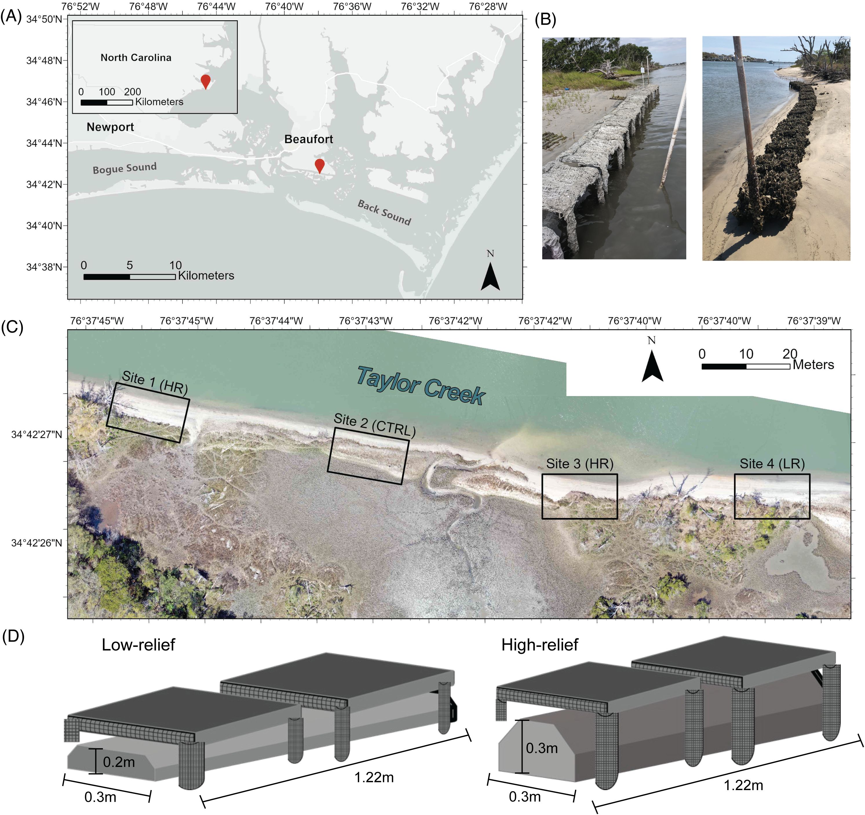
Figure 1. (A) Map showing study site location within the Rachel Carson Reserve along Taylor Creek in North Carolina (marked by red pin). (B) Images of Oyster Catcher™ reefs immediately post-installation in 2020 (left) and after oyster recruitment in 2022 (right). (C) Study site area before oyster reef installation in 2020 (imagery captured using a drone on April 6, 2020 for pre-construction assessment). Site areas are within the black rectangles. (D) Diagram of Oyster Catcher™ reefs.

We conducted this study on three engineered oyster reefs and one control site with no oyster reef. Two of the oyster reefs measured 12m*2m*0.3m (length x width x height) and one measured 12m*2m*0.2m (Figure 1D). All sites, including the control site (CTRL), were 12m in length. Hereinafter, the oyster reefs with a height of 0.3m above the sediment surface will be referred to as high-relief (HR) reefs, and the oyster reef with a height of 0.2m above the sediment surface will be referred to as a low-relief (LR) reef. These two heights were chosen because they are in the range of elevations that are optimal for oyster growth in the Rachel Carson National Estuarine Research Reserve (Fodrie et al., 2014; Ridge et al., 2015). Taylor Creek is dredged for boat passage, and it was dredged during the study period in March of 2022. All three reef sites lacked low marsh but all sites including the control site had a landward high marsh consisting mostly of Juncus roemerianus (black needlerush). The control site also had a section of low marsh with Spartina alterniflora (also known as Sporobolus alterniflorus) as the dominant vegetation type.

We collected wave energy, sediment composition, oyster abundance and height, reef surface complexity, and slope data to characterize the study sites (Table 1, see Supplementary Material for methods). The average wave height was similar across all sites, with an average wave height of 0.92cm in 2021 (±0.55cm, p =0.08, Table 1). Along the marsh edge, the ratio of mud to sand was similar in 2021 and 2023 (Supplementary Figure 1). The average mud percentage across sites with engineered oyster reefs was 2.95% (± 0.99%) while the average mud percentage at the control site was 6.78% (± 1.48%; Table 1). Oyster abundances and lengths were higher at sites 1 (HR) and 3 (HR) when compared to site 4 (LR) (p<0.01; Supplementary Figure 2). We calculated a steeper drop off in elevation seaward of the oyster reefs at sites 1 (HR), 2 (CTRL), and 4 (LR) 13°, 11° and 16°, respectively) while site 3 (HR) is characterized by a more gradual decline in elevation (2°) (Table 1; Supplementary Figure 4). However, these bathymetric data were collected prior to oyster reef installation, and the authors qualitatively observed the seaward slope increase in steepness at sites 1 (HR), 2 (CTRL), and 4 (LR) after oyster reef installation. Water levels during the study period (March 2, 2022 – April 18, 2023) were slightly lower (1.3cm) than expected based on trends from the previous 10 years (March 2, 2012 – March 1, 2022).

Table 1

Table 1. Site characteristics.

2.2 RTK-GNSS and drone data

We surveyed Ground Control Points (GCPs) using RTK-GNSS to align drone imagery with real-world XYZ coordinates. To increase accuracy, we created a survey-grade benchmark using the Trimble Spectra Precision SP80 system, which has a high-precision static post-processed accuracy of 3mm horizontally and 3.5mm vertically (Root Mean Squared Error [RMSE]) (SP80 manual, 2019). For benchmarking, we collected data continuously in 1-second intervals for a minimum of 2 hours. The ground-level GCPs consisted of orange squares with a black border and central X hammered flush to the ground with a surveyor’s nail. In 2022, we also included elevated GCPs, consisting of a rebar staked into the ground with an orange square cap placed securely on top, and in 2023, our elevated GCPs consisted of raised PVC pipes driven into the ground with blue disks screwed to the top. We placed the elevated GCPs seaward of the oyster reefs at heights comparable to the reefs to enhance georeferencing around the oyster reefs. We recorded a total of 4 elevated and 18 ground-level GCPs in 2022, and in 2023, we recorded 6 elevated and 11 ground-level GCPs (Supplementary Table 1). The SP80 receiver was placed over the center of each GCP, recording 1-second intervals at 60 fixed epochs. The overall (XYZ) benchmark RMSE for each year is shown in Table 2. To estimate total positional uncertainty, we conservatively added the benchmark RMSE (base station error), horizontal rover precision, and vertical rover precision for each survey, as shown in Table 2. This resulted in total RTK-GNSS uncertainties of 0.021 m in 2022 and 0.022 m in 2023.

Table 2

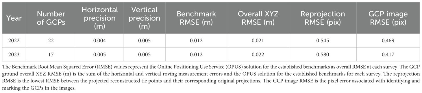
Table 2. Errors used when assessing GCP error and generating precision estimates and number of GCPs collected each year along with the RTK-GNSS maximum horizontal and vertical standard deviations (roving measurement error).

After surveying GCPs using RTK-GNSS, we conducted drone flights using a DJI Phantom 4 Pro with a 1” CMOS Red-Green-Blue sensor. Federal Aviation Administration Part 107 certified remote pilots operated all flights. Wind speeds were monitored to ensure they were below 15 mph for flight safety and to minimize motion blur in the images. Optimal flight times relative to the predicted Mean Lower Low Water (MLLW) tide were determined using the Beaufort, Taylor Creek, NC station (ID: 8656518) (NOAA) (Supplementary Figure 5). Flights were scheduled near MLLW to maximize topographic exposure; however, environmental conditions could not be fully standardized due to tidal and weather constraints. Variations in predicted low tide levels and cloud cover were unavoidable, but surveys were conducted around the same time of year: March 2, 2022 and April 18, 2023 – to maintain temporal consistency. Flight plans were created using DJI Ground Station Pro with consistent settings across years: 15 m altitude, gimbal pitch angle of -60°, a front overlap ratio of 75%, side overlap ratio of 80% to reduce error (Nesbit and Hugenholtz, 2019). Each survey included two crosshatch flights, one at 30°course angle and another at 90°. We used an oblique gimbal pitch angle because when combined with a crosshatch pattern flight, image geometry is enhanced which reduces systematic error in the DEMs (Nesbit and Hugenholtz, 2019). To help minimize motion blur, photos were captured while hovering at each waypoint. Flights covered 0.26 ha at 4.7 m/s, capturing a total of 182 waypoints across both years. Drone flights were conducted for pre-construction site assessment, but these were not included due to differing global navigation systems used which led to a higher overall RMSE than that of the data included in this study.

2.3 Drone data processing and analyses

2.3.1 Drone imagery data processing

We used SfM photogrammetry in Agisoft Metashape Pro (v. 1.8.3) to generate DEMs and orthomosaics for assessing topographic changes and delineating the marsh edge. Our workflow followed principles outlined by Cooper et al. (2021) and Guan et al. (2022) but incorporated some modifications given our unique study site. To minimize the impact of poorly focused imagery on image alignment, we used the automatic image quality feature to exclude images with a quality lower than 0.6 units. We then matched overlapping image features into tie points using the “align images” function with a key point limit of 40,000 and tie point limit of 4,000. Tie points with reprojection errors greater than 0.7, 0.5, and 0.3 were tested and filtered to eliminate outliers. The threshold that most effectively improved our accuracy was 0.3. For quality control, we optimized the initial image network based on the lowest RMSE between the projected reconstructed tie points and their corresponding original projections (i.e., reprojection RMSE, as shown in Table 2). All GCPs were identified and marked on the images using a combination of guided and manual approaches, providing further quality control for determining GCP RMSE in pixels (GCP image RMSE shown in Table 2).

We then used the RTK-GNSS data collected for each GCP to georeference the images to the North American Datum of 1983 (NAD83) (2011), UTM Zone 18N (EPSG:6318), with elevations referenced to the North American Vertical Datum of 1988 (NAVD88) using the Geoid 18 model accompanied by a bundle adjustment using all GCPs as control. All bundle adjustments were performed using the camera parameters of focal length (f), principal point (cx, cy), and radial distortion (k1, k2, k3). Since the principle of Monte Carlo simulation follows the law of large numbers theorem by averaging the results of different GCPs over many trial runs, it provides a more reliable result of the expected elevation error (Cooper et al., 2021). Therefore, we adopted the Monte Carlo approach by James et al., 2012, simulating 100 iterations using a random subset of 70% of GCPs as control to build the model and a 30% subset as quality checkpoints to assess the accuracy of the model. This method was used to quantify the final XYZ error as one standard deviation (SD) for our SfM-derived products. A dense point cloud was generated and filtered to isolate ground points, which formed the basis for creating our DEMs. This filtering process involved manual classification and subsequent visual inspection. We then used the DEMs to generate the orthomosaics. Our DEMs from 2022 and 2023 had resolutions of 0.88 cm² and 0.98 cm², and our orthomosaics had resolutions of 0.44 cm² and 0.49 cm².

2.3.2 Image analysis and classification

To define the marsh edge where it transitions into foreshore topography, we applied digital image analysis and manual classification techniques. We used image segmentation to delineate the marsh edge, which supports reproducible shoreline mapping and enables consistent assessment of horizontal marsh retreat or expansion over time (e.g., Sirianni et al., 2022). We implemented image segmentation in ArcGIS Pro (v. 3.2) using the Segment Mean Shift (Spatial Analyst) algorithm to group pixels with similar spectral characteristics into segments (Comaniciu and Meer, 2002). Through trial and error, we selected optimal parameters for the algorithm: 20 for spectral detail, 9 for spatial detail, and a minimum segment size of 3,000, given the sub-centimeter fine resolution drone orthoimagery (0.44 cm² and 0.49 cm² per pixel).

After image segmentation, we overlaid the DEM, orthomosaic, and segmented image in ArcGIS Pro to manually classify each image segment into habitat types, including sandflat, water, low marsh, and high marsh. Classifications were conducted at visual scales ranging from 1:15 to 1:100 using our sub-centimeter resolution drone orthoimagery, informed by extensive field knowledge and on-site observations. For consistency and to reduce classification errors, all classifications were conducted by a single researcher using standard decision rules. We then converted the classified marsh polygons to line features representing the marsh edge. The resulting marsh edge delineation at each spatial scale used in the classification process is demonstrated in Supplementary Figure 6, showing how segmentation and manual labeling were applied to generate reproducible and reliable shoreline boundaries.

2.3.3 Horizontal marsh edge movement

The changes in the horizontal position of the high marsh edge were assessed using the software package Analyzing Moving Boundaries Using R (AMBUR) (Jackson et al., 2012; Polk and Eulie, 2018; Polk et al., 2021). AMBUR generates transects between two baselines and uses the end point rate (EPR) to calculate the change between two marsh edge positions (Jackson et al., 2012). The End Point Rate Tool for QGIS and the Digital Shoreline Analysis System (DSAS) are also useful tools for calculating EPR, but they do not allow the use of two baselines for generating transects (Terres De Lima et al., 2021; Himmelstoss et al., 2018). In addition, AMBUR allows users to “filter” transects to reduce issues related to crisscrossing transects along irregular shorelines (Jackson et al., 2012). Because of the irregularity of the marsh edge delineations caused by the small pixel size of the orthomosaics, we selected AMBUR to ensure accurate EPR calculations using both an inner and outer baselines and utilizing the “filter” feature. We used a transect spacing of 1m and created inner and outer baselines for each site’s marsh edge using the buffer tool in ArcGIS Pro. Though it is generally advised to use a transect spacing slightly greater than the resolution of your imagery, we chose a transect spacing of 1m to align with the methodologies of other studies in our region to allow for comparisons of our results (Polk and Eulie, 2018; Polk et al., 2021). The rate of change is equal to the change in horizontal edge positions divided by the time elapsed between the two marsh edges, with positive values indicating expansion seaward and negative values indicating retreat (Fletcher et al., 2003; Cowart et al., 2010; Currin et al., 2015). We calculated the EPR error using the following formula:

$\begin{array}{ll}\text{EPR error}=\frac{\sqrt{{(h unc A)}^2+{(h unc B)}^2}}{elapsed time}& (1)\end{array}$

where, in our case, h unc A is the Monte Carlo horizontal RMSE of 2022 (± 5.99cm) and h unc B is the Monte Carlo horizontal RMSE of 2023 (± 3.47cm), and elapsed time is the time between the data collected in 2022 and the data collected in 2023 (1.13 years) (Jackson et al., 2012). We calculated horizontal marsh edge migration results in 3 ways; one in which all transects are included in the analysis, one in which transects within the EPR error were converted to a value of zero to indicate that no significant change had occurred, and one in which transects within the 95% confidence interval (CI) of the EPR error were converted to zero. We calculated the mean EPR value for each site to determine the average high marsh edge migration rate.

2.3.4 Volumetric changes

The influence of engineered oyster reefs on the development of the foreshore topography can be assessed using the DEM of Difference (DoD) approach, which is used in various morphological change detection studies (e.g., Lane et al., 1994; Wheaton et al., 2010; James et al., 2017; Sirianni et al., 2024). The DoD approach involves subtracting the older DEM from a newer DEM using the following equation:

$\begin{array}{ll}\text{DoD}=\text{DEM}2-\text{DEM}1& (2)\end{array}$

where in our case, DEM2 is the 2023 DEM and DEM1 is the 2022 DEM. To isolate changes specific to intertidal zones, we applied the habitat map as a mask, extracting areas classified as sandflat for analysis. Before subtracting our DEMs, we resampled the DEM with the lower cell size (0.88cm²) to the DEM with the higher cell size and alignment, resulting in a matching and aligned resolution of 0.98cm².

To determine significant elevation changes in the DoD analysis, we applied four minimum critical threshold approaches to account for elevation uncertainty. First, we consider the annualized Monte Carlo simulated vertical precision estimate as a SD (3.79 cm, the largest vertical uncertainty between the two surveys), which is assumed to follow a normal distribution and is equivalent to the RMSE. Based on this assumption, we also apply a more conservative approach to estimate the linear error at the 95% CI (LE95) by multiplying the Monte Carlo error by 1.96, following guidelines by the National Standards for Spatial Data Accuracy (FGDC, 1998; Cooper et al., 2013). We determined this minimum threshold by multiplying the Monte Carlo simulated error $(M{C}_{\sigma })$ by 1.96:

$\begin{array}{ll}LE95=1.96\times M{C}_{\sigma } & (3)\end{array}$

The third approach provides a more robust estimate because it calculates the minimum level of detection (_minLOD) by incorporating error from both DEMs used in the DoD analysis. We calculated the _minLOD using the following equation:

$\begin{array}{ll}{ }_{min}\text{LOD}=\sqrt{\frac{{(v unc A)}^2+{(v unc B)}^2}{elapsed time}}& (4)\end{array}$

where v unc A is the Monte Carlo vertical RMSE of the 2022 DEM (± 4.29cm) and v unc B is the Monte Carlo vertical RMSE of the 2023 DEM (± 3.53) (Fuller et al., 2003). The final approach builds on the LE95 and _minLOD by applying the 95% CI (CI95) of the _minLOD (Wheaton et al., 2010). We calculated this threshold using:

$\begin{array}{ll}CI95=1.96\times \min LOD& (5)\end{array}$

To assess significant elevation changes, we applied each uncertainty threshold to the DoD grid. Cells with elevation differences within +/-uncertainty were set to zero, indicating no significant change had occurred. We then multiplied the DoD grid cell values by their respective cell area to estimate erosion (negative values) and deposition (positive values) volumes of the nearshore topography for each oyster reef and reference site. To standardize comparisons, we divided the total erosion, deposition, and net volumetric change by the site area to obtain an average measure of sediment redistribution at each site.

2.4 Statistical analyses

We conducted Kruskal-Wallis tests and Dunn’s tests to determine if net volumetric changes varied significantly between site or uncertainty threshold used. We used one-way ANOVAs and Tukey’s post-hoc test to determine if EPRs were significantly different between sites or uncertainty thresholds.

3 Results

3.1 Horizontal marsh edge movement

Marsh edge retreat was observed across all sites (Table 3). The magnitude of marsh edge retreat was not significantly different across sites. At site 1 (HR), site 2 (CTRL), site 3 (LR), and site 4 (HR), the marsh edge retreated by 0.29 ± 0.42 m/year, 0.35 ± 0.32 m/year, 0.48 ± 0.24 m/year, and 0.38 ± 0.39m/year, respectively. There was no significant difference between average marsh edge retreat values calculated using different uncertainty thresholds (no transects removed, transects within the EPR error removed (±5.60cm), and transects within the 95% CI of the EPR error removed (±10.97cm) (p = 0.9998). Across all sites, the marsh retreated an average of 0.38 ± 0.34 m/year.

Table 3

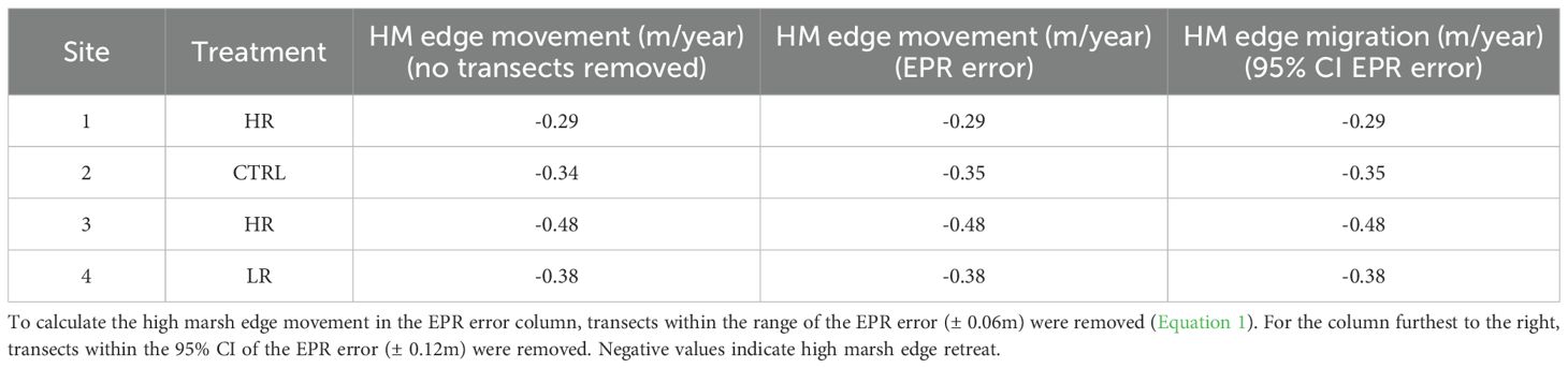
Table 3. Annualized high marsh (HM) edge movement.

3.2 Elevation and volumetric changes

Using the _minLOD uncertainty threshold (uncertainty ±4.91 cm), all sites except site 4 (LR) experienced net volumetric losses (Table 4). Site 2 (CTRL) experienced the greatest average net volumetric loss (-6.91 cm/year), followed by site 1 (HR) (-5.65 cm/year). Net volumetric changes were significantly different between each site (p<0.01). Site 3 (HR) experienced the most average deposition of sediment (0.17 cm/year), but not enough to offset losses. Site 4 (LR) experienced no net volumetric change (0.00 cm/year). Site 2 (CTRL) had the greatest percent area of erosion at 98% while site 4 (LR) eroded at only 4.2% of the total area.

Table 4

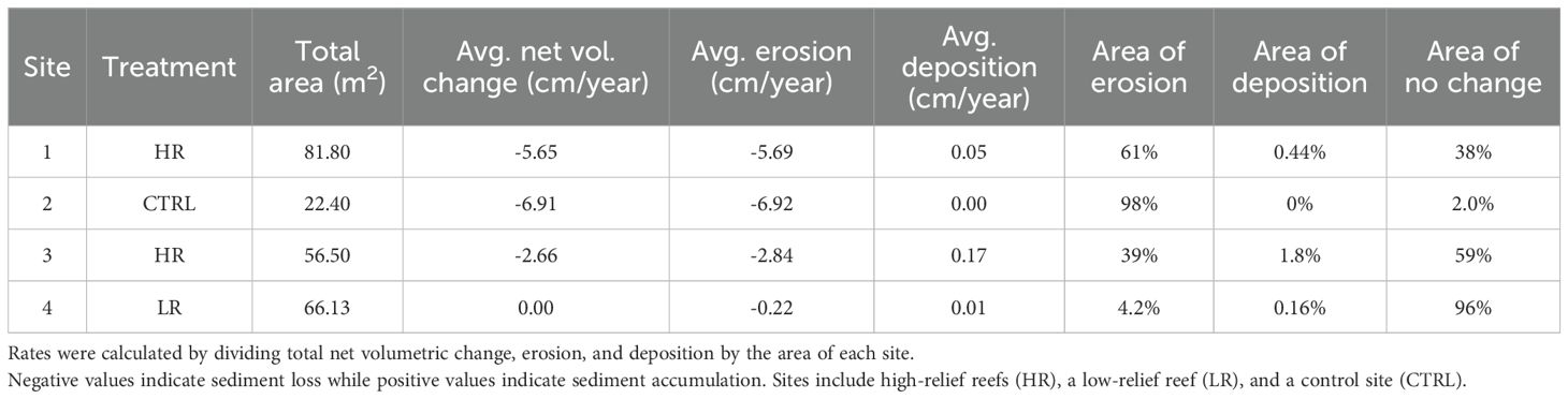
Table 4. Metrics calculated for each site using the DEM of difference (DoD) (Equation 2) created using the _minLOD uncertainty threshold (uncertainty ±3.80cm) including total area analyzed, annualized average net volumetric change, erosion, and deposition.

By observing the DoD, we can see that the greatest loss of elevation at site 1 (HR) occurred along the marsh edge (0.1-0.2cm/year), whereas the highest concentration of elevation loss at site 3 occurred on the west side of the reef (0.06-0.1 cm/year) as shown in the map (Figure 2). Site 3 (HR) had some increase in elevation just landward of the reef (0.06-0.1 cm/year). Site 2 (CTRL) had a loss in elevation across the entire site (0.1-0.2 cm/year), and site 4 (LR) held a relatively constant elevation from 2022 to 2023.

Figure 2

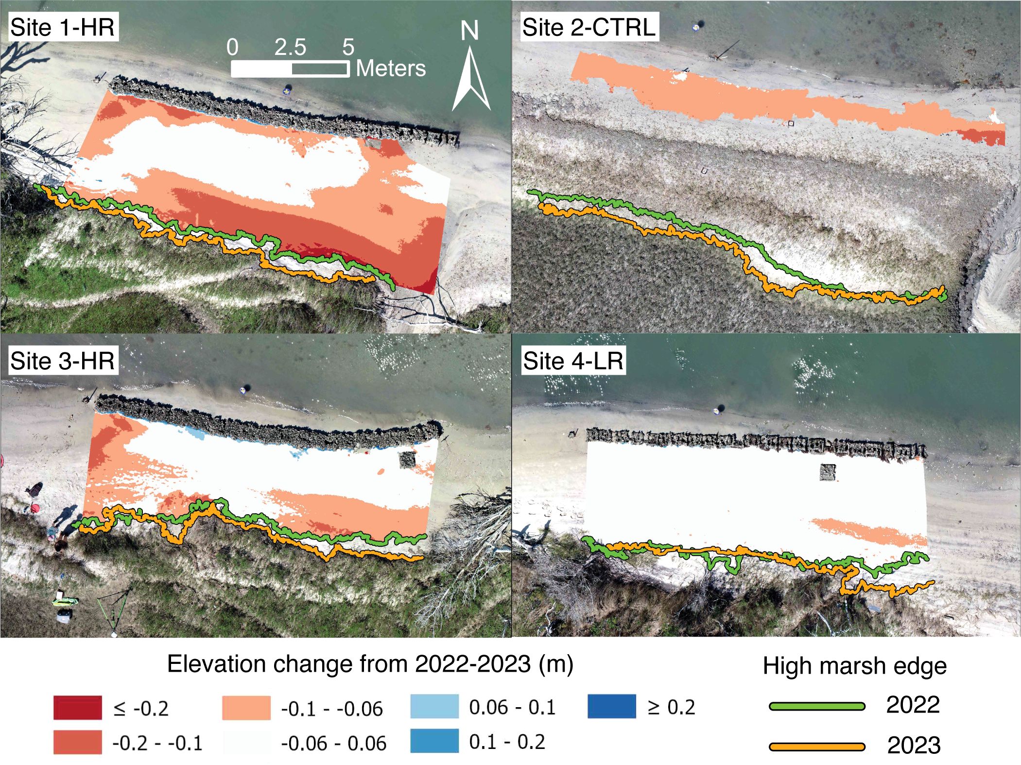
Figure 2. Elevation changes for the foreshore topography at each site. Elevation loss is shown in red while elevation gain is shown in blue, and non-significant change is shown in white. The high marsh edge for each site is depicted using a green line for 2022 and a yellow line for 2023. The background imagery is the orthomosaic from 2023. The top left panel shows site 1 (a high-relief site), the top right panel shows site 2 (our control site), the bottom left panel shows site 3 (a high-relief site), and the bottom right panel shows site 4 (a low-relief site). All marsh grass and water has been filtered from the analysis.

Applying different levels of uncertainty to our DoD resulted in variable estimates of net volumetric change, erosion, and deposition rates at each site (Table 5). Our annualized uncertainty thresholds for $M{C}_{\sigma }$, LE95, _minLOD, and CI95 were ±3.79cm, ± 7.44cm, ± 4.91cm, and ±9.63cm, respectively. The estimates of net volumetric change using different uncertainty thresholds were significantly different (p<0.01). Using the most conservative uncertainty threshold (CI95) resulted in the lowest estimates of net volumetric change, erosion, and deposition. This is most notable at site 2 (CTRL) where applying the $M{C}_{\sigma }$ uncertainty resulted in an average erosion rate of -6.99cm³/year but applying the CI95 uncertainty resulted in an erosion rate of only -0.31 cm³/year.

Table 5

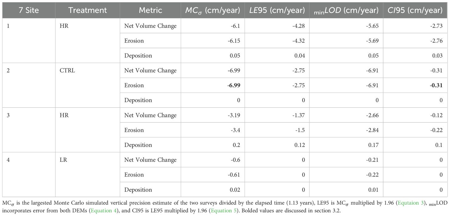
Table 5. Annualized average net volumetric change, erosion, and deposition rates calculated using different vertical uncertainties as the thresholds for the minimum level of detection (MCσ, LE95, _minLOD, and CI95).

The level of uncertainty used in DoD impacts how much detected change is retained or filtered out, as shown in Figure 3. The DoD without uncertainty filtering (demonstrated using site 1 and shown in Figure 3A) captures the most elevation change in red but includes differences within the DEM error margin, potentially overestimating volumetric change (Rumsby et al., 2008). Applying $M{C}_{\sigma }$ (Figure 3B), _minLOD (Figure 3D), and LE95 (Figure 3C) progressively removes areas with higher uncertainty. However, CI95 (Figure 3E) applies the strictest threshold, filtering out subtle changes. Wheaton et al. (2010) note that higher uncertainty thresholds such as CI95 result in more conservative estimates of erosion and deposition volumes. While this approach reduces false positives, it may also exclude small but ecologically meaningful changes in elevation. This could be problematic in short-term monitoring where detecting fine-scale sediment changes is needed to understand shoreline and habitat change (Duffy et al., 2018).

Figure 3

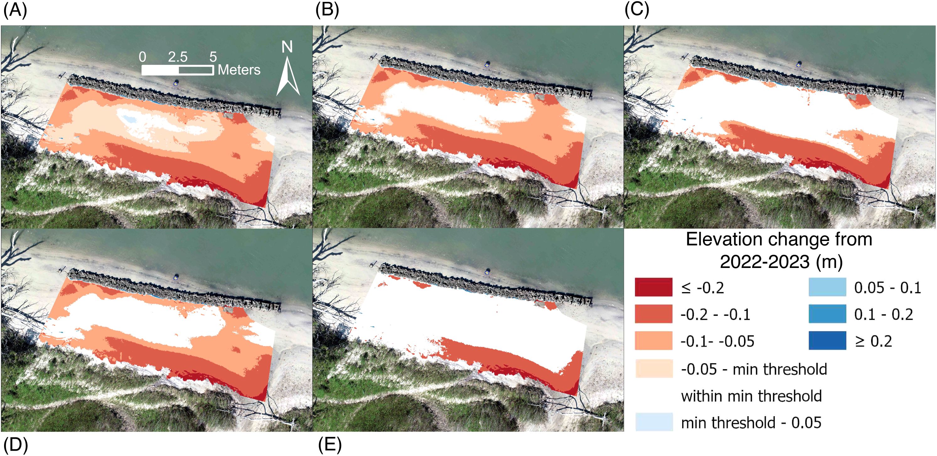
Figure 3. Using site 1 as an example, this figure shows DoDs with different levels of uncertainties used as thresholds for the minimum level of detection; (A) no uncertainty, (B) $M{C}_{\sigma }$, (C) LE95, (D) _minLOD, e) CI95 where (A) applied no uncertainty threshold, (B) applied the greater uncertainty threshold of the two DEMs calculated from the Monte Carlo simulation, (C) applied the 95% CI of the greater uncertainty threshold of the two DEMs calculated from the Monte Carlo Simulation, (D) applied the uncertainty threshold calculated using the _minLOD formula, and (E) applied the 95% CI of the _minLOD. The area within the minimum level of detection for each figure is shown in white.

4 Discussion

Our results revealed that the marsh edge eroded at all engineered oyster reef sites as well as the control site, and elevation declined at all sites except the low-relief engineered oyster reef site from 2022-2023. These results suggest that significant changes to the topography were occurring at our sites 2–3 years post restoration. Applying different uncertainty thresholds to marsh edge movement calculations and volumetric change analyses resulted in similar marsh edge retreat values but significantly different volumetric change values. More conservative uncertainty thresholds (95% CI) produce more robust results but may filter out some ecologically important changes in short-term monitoring projects.

4.1 Marsh edge vs. volumetric erosion

The marsh edge eroded at all sites regardless of reef presence. This is likely due to tidal currents caused by the 0.86m tidal range in Taylor Creek (NOAA, 2025), marsh drainage canals located between site 1 and 2 and between sites 2 and 3, and potentially due to elevation drop-off seaward of the oyster reefs (Supplementary Figure 1). Although elevation has stayed consistent at site 4 (LR), the marsh edge retreated substantially, indicating that the oyster reef at this site is not protecting the marsh edge. However, it is possible that sediment losses from the eroding marsh edge are being trapped by the oyster reef, resulting in no net change in elevation at the site. The reef at site 4 was constructed at a lower height than the reefs at site 1 and 3, which could explain its ability to trap sediments more efficiently. In contrast, sites 1 and 3 displayed a net loss of elevation from 2022 to 2023. Some of the elevation losses could have been a product of initial sediment accretion and then redistribution qualitatively observed immediately post-construction of the reefs from 2020 to 2021 (R. Gittman, personal observation), however, due to logistical constraints, we were unable to quantify changes within the first year using the methods described in this study. Both sites 1 and 3 displayed elevation loss near the eastern side of the marsh edge which could be due to tidal current patterns. The elevation loss on the eastern side of site 3 could also be due to the marsh drainage canal between sites 2 and 3. However, site 1 experienced elevation loss directly landward of the oyster reef while site 3 did not. This could be due to differences in seaward bathymetry as the elevation decline seaward of site 1 is much steeper than the elevation decline at site 3 and/or due to scouring caused by interactions between the oyster reef and tidal currents. Site 1 also experienced high rates of marsh edge retreat and elevation loss along the marsh edge in the western region. This is likely due to a combination of factors including the tidal current velocities and the marsh drainage canal located just west of the marsh edge. It is also possible that the close proximity of the oyster reefs to each other influenced hydrodynamic patterns around the sites and caused erosion. It is important to note that this study lacks pre-restoration monitoring which limits our ability to conclude that marsh and sediment changes are due to reef installation. Future studies should incorporate pre-restoration monitoring to determine the influence of reef installation on erosional patterns. Our results indicate that topographic changes can occur even 2–3 years post installation of shore-protection structures. This highlights the need for long-term monitoring of shore stabilization projects to evaluate performance (see Baker and Gittman, 2024).

Our measured marsh edge retreat measurements in the control and engineered oyster reefs are similar to other values reported in North Carolina at unprotected marshes behind living shorelines. Polk and Eulie, 2018 measured marsh edge retreat at rates of -0.16 ± 0.82 m/year and -0.37 ± 0.16m/year after installation of living shorelines and -0.55 ± 0.82 m/year and -0.67 ± 0.16 at control sites in Carteret County, NC. In this study, horizontal marsh edge movement results using different error thresholds were not statistically significant from each other (p = 0.9998). To provide a more conservative estimate of marsh edge movement, we recommend filtering out transects within the 95% CI of the measure of uncertainty by converting these values to zeros. However, in regions with smaller rates of marsh edge movement, it may be beneficial to apply a less conservative uncertainty threshold to detect areas of marsh edge retreat.

Few studies have monitored elevation changes near living shorelines. However, Smith et al., 2018 monitored elevation landward and seaward of unprotected marshes and living shorelines and found that the elevation at unprotected marshes remained consistent across a 2-year period, while elevation landward of living shorelines increased. This is in contrast to our results which indicated that elevation declined at all sites except our low-relief oyster reef site. Differences in site conditions, including wave energy, alongshore currents, slope, and vegetation coverage, as well as living shoreline designs and substrates likely contribute to differences in observed shoreline changes (see Polk and Eulie, 2018).

Though time-intensive, creating DEMs and orthomosaics with sub-centimeter resolutions using drones and SfM can assist with evaluating NbS (Kumar et al., 2021). Most NbS projects are funded for short-term periods (2–5 years) (Kumar et al., 2021, O’Leary et al., 2023). As such, to accurately evaluate the success of NbS, it is necessary to detect small-scale changes that may occur over small time-scales. High-resolution products can also assist practitioners in detecting spatial patterns of elevation change during ambient conditions or after storm events. For example, DEMs and orthomosaics may reveal erosion hot spots which is useful information for implementing adaptive management. Detecting changes at a centimeter level allows managers to implement NbS before erosion reaches meter-level magnitudes. High-resolution data is also necessary for comparing the coastal protection properties of different NbS as differences in protection may be minimal but ecologically or economically important.

Despite the availability of more sophisticated error-handling techniques, DoD remains widely used due to its efficiency. More advanced methods such as Monte Carlo simulation on DEMs (Oksanen & Sarjakoski, 2005) and point clouds (Cooper et al., 2021) provide improved uncertainty handling. However, these computationally intensive methods require specialized skills, which might make them less practical for certain routine monitoring efforts. It is best practice to consider high levels of uncertainty filtering (e.g., CI95) to extend confidence in detected changes. However, current limitations in vertical accuracy (i.e., at the centimeter level) make their application challenging in short-term monitoring. In this study, the RTK-GNSS benchmarks had overall XYZ uncertainties of 0.021 and 0.022 m at each site (see Table 2), and this error was appropriately carried into the SfM data processing. The inherent limitations of current GNSS technology mean that uncertainty at the centimeter level persists throughout the dataset. This makes it difficult to detect sub-centimeter-scale changes over short monitoring periods with high confidence. Stricter thresholds are beneficial for long-term studies to isolate the most significant changes. However, applying these thresholds over short time scales, where volumetric change is already minimal, filtered out nearly all detectable erosion and deposition in this short-term study. Future research should evaluate whether uncertainty thresholds disproportionately filter out subtle, spatially structured changes associated with real geomorphic or ecological processes, particularly in short-term monitoring contexts.

4.2 Site characteristics

To contextualize changes occurring around living shorelines, it is important to report site characteristics including wave energy, sediment composition, shoreline slope, oyster reef surface complexity, and oyster abundances (Bredes et al., 2024; Tweel et al., 2025; Baggett et al., 2015). Environmental wave energy can influence the ability of living shorelines to trap sediment (Palinkas et al., 2022). High wave energy may result in continued erosion of the shoreline while low energy can result in sediment trapping. However, wave energy must be high enough to transport sediment landward of the living shoreline (Davis et al., 2015; Jackson et al., 2002). Analyzing sediment grain size and shoreline slope can help to contextualize patterns of erosion and accretion (Palinkas et al., 2023; Polk and Eulie, 2018). Fine sediments often indicate low wave energy and sediment accretion while larger grain sizes often indicate high wave energy and erosion (Visher, 1967). Lastly, metrics of oyster reef complexity influence flow thereby influencing sedimentation rates (Styles, 2015). Oyster reefs can reduce incoming wave energy which allows lower rates of erosion and higher rates of sediment accretion (Wiberg et al., 2019).

In this study, we characterized sites by collecting data on recommended metrics including wave heights, sediment composition, landward and seaward shoreline slope, reef surface complexity, and oyster abundances and lengths (Bredes et al., 2024; Baggett et al., 2015). Due to the short duration of our study period, we were unable to make conclusions about how these characteristics may be influencing marsh edge movement and volumetric changes. We did not collect data on tidal current velocities. To assess the performance of shoreline stabilization features, it is critical to understand the processes influencing erosion and accretion patterns. Because of this, future living shoreline studies should monitor for longer durations and incorporate tidal current velocity to monitor seaward slopes (Baker and Gittman, 2024; Wang et al., 2023; Bredes et al., 2024).

4.3 Drone imagery and SfM for living shoreline monitoring

As demonstrated in this study, drone imagery and SfM photogrammetry can provide high resolution data for monitoring the coastal protection properties of living shorelines. However, there are several challenges associated with drones and SfM techniques. For example, the tidal levels of our flights were not exactly the same across years which resulted in higher water levels in 2022. Though this area was filtered out of analyses, it meant we were unable to measure erosion or deposition in these areas (see areas with no elevation change coloring in Figure 2). Because our site was located in a nature preserve accessible to the public, we were unable to place permanent benchmarks to verify elevation across years at the same location. In environments less accessible by the public, fixed benchmarks (e.g., survey nails or an existing structure) can provide a valuable control for repeat elevation and vertical accuracy checks.

Overall, this study demonstrates that drones and SfM techniques are valuable tools for assessing the performance of different living shoreline structures when appropriate uncertainty thresholds and site conditions are considered. Managers and practitioners should consider the benefits and drawbacks of using different levels of uncertainty when monitoring vertical and horizontal changes, as more conservative thresholds (e.g., CI95) reduce the risk of interpreting noise as real change but may also filter out subtle yet ecologically meaningful changes in short-term monitoring. When installing new living shoreline structures, it is important to consider site characteristics when selecting substrates and designs. For example, while elevation remained stable at the low-relief reef site, marsh edge retreat occurred across all sites, demonstrating the complexity of site-specific responses. More long-term studies are needed to evaluate the use of novel living shoreline structures in varying environmental conditions, and future research should incorporate hydrodynamic data such as tidal currents and seaward slope to provide context for understanding the patterns observed in the drone-derived data.

In addition to post-construction monitoring, drone-based surveys offer powerful tools for pre-construction assessments by enabling high-resolution mapping of elevation, slope, and land cover to inform site selection and design. Pre-construction data are critical for avoiding impacts to ecologically valuable habitats and for establishing robust baselines for change detection. However, as Baker and Gittman (2024) highlighted, most living shoreline projects lack co-funded monitoring at the planning stage, limiting the ability to rigorously evaluate ecological and geomorphic outcomes. This study reflects that challenge, as no pre-restoration data with comparable horizontal resolution and vertical accuracy were available to detect fine-scale changes. This limitation underscores the need to prioritize high-resolution baseline surveys, particularly with drone-based methods. Future efforts should prioritize co-funded pre-restoration drone surveys with in-situ observations to support more rigorous before–and–after comparisons and better link observed outcomes to site characteristics and intervention types.

Data availability statement

The datasets presented in this study can be found in online repositories. The names of the repository/repositories and accession number(s) can be found below: Open Science Foundation (OSF) data repository, accession DOI 10.17605/OSF.IO/SJVPN.

Author contributions

MG: Writing – original draft, Formal analysis, Visualization, Methodology, Conceptualization, Investigation. GT: Writing – review & editing, Investigation, Methodology, Formal analysis. HS: Methodology, Investigation, Writing – review & editing, Funding acquisition. SN: Funding acquisition, Writing – review & editing. CB: Funding acquisition, Writing – review & editing. PM: Writing – review & editing, Funding acquisition. BP: Writing – review & editing. JR: Writing – review & editing. RG: Writing – review & editing, Methodology, Funding acquisition.

Funding

The author(s) declare financial support was received for the research and/or publication of this article. This project is funded, in part, by the US Coastal Research Program (USCRP) as administered by the US Army Corps of Engineers^® (USACE), Department of Defense and National Sea Grant, as administered by the National Oceanographic and Atmospheric Administration (NOAA) (Grant #s W912HZ2120010 and NA23OAR4170122-T1-01). Initial site characteristics monitoring was funded by a North Carolina Sea Grant (NCSG) Community Collaborative Research Grant (CCRG) (Grant # 2011-1590-08 20-CCRG-02) in partnership with the North Carolina Coastal Reserve and NOAA National Estuarine Research Reserve and the NC Policy Collaboratory (Grant #s 20170 12593–221010 and 20170 12593–221010 KOAST). Geesin's participation was supported by funding from the National Science Foundation Coastal Community Environmental Science Data Scholars National Research Traineeship (grant # DGE-2125684) and from the North Carolina Sea Grant-Space Grant graduate research fellowship. Dr. Narayan’s time on this work was supported by National Science Foundation DISES grant #2206479. The oyster reef construction was funded by the U.S. Fish and Wildlife Service (USFWS) Atlantic Coast fish Habitat Partnership (ACFHP) (Grant # F19AP00230) and construction materials and labor were provided by Sandbar Oyster Company and East Carolina University. The authors acknowledge the USACE, NOAA, Sea Grant, and USCRP’s support of their effort to strengthen coastal academic programs and address coastal community needs in the United States.

Acknowledgments

Thank you to Anna Albright, James Kelley, Ryann Knowles, Philip Van Wagoner, Jenny Fickler, Charles Brooks III, Chiante Brown, and the Gittman lab for their assistance with monitoring and sample collection.

Conflict of interest

The authors declare that the research was conducted in the absence of any commercial or financial relationships that could be construed as a potential conflict of interest.

Generative AI statement

The author(s) declare that no Generative AI was used in the creation of this manuscript.

Any alternative text (alt text) provided alongside figures in this article has been generated by Frontiers with the support of artificial intelligence and reasonable efforts have been made to ensure accuracy, including review by the authors wherever possible. If you identify any issues, please contact us.

Publisher’s note

All claims expressed in this article are solely those of the authors and do not necessarily represent those of their affiliated organizations, or those of the publisher, the editors and the reviewers. Any product that may be evaluated in this article, or claim that may be made by its manufacturer, is not guaranteed or endorsed by the publisher.

Author disclaimer

Any opinions, findings, and conclusions or recommendations expressed in this material are those of the authors’ and do not necessarily reflect the views of the National Science Foundation. The content of the information provided in this publication does not necessarily reflect the position or the policy of the government, and no official endorsement should be inferred.

Supplementary material

The Supplementary Material for this article can be found online at: https://www.frontiersin.org/articles/10.3389/fevo.2025.1616227/full#supplementary-material

References

Adade R., Aibinu A. M., Ekumah B., and Asaana J. (2021). Unmanned Aerial Vehicle (UAV) applications in coastal zone management—a review. Environ. Monit. Assess. 193, 154. doi: 10.1007/s10661-021-08949-8

PubMed Abstract | Crossref Full Text | Google Scholar

Attard M. R. G., Phillips R. A., Bowler E., Clarke P. J., Cubaynes H., Johnston D. W., et al. (2024). Review of satellite remote sensing and Unoccupied Aircraft Systems for counting wildlife on land. Remote Sens. 16, 627. doi: 10.3390/rs16040627

Crossref Full Text | Google Scholar

SP80 GNSS Receiver. Available online at: https://trl.trimble.com/docushare/dsweb/Get/Document-844535/SG-SP80-Br-v2.pdf (Accessed March 7 2025).

Google Scholar

Baggett L. P., Powers S. P., Brumbaugh R. D., Coen L. D., DeAngelis B. M., Greene J. K., et al. (2015). Guidelines for evaluating performance of oyster habitat restoration. Restor. Ecol. 23, 737–745. doi: 10.1111/rec.12262

Crossref Full Text | Google Scholar

Baker R. and Gittman R. K. (2024). Co-funding robust monitoring with living shoreline construction is critical for maximizing beneficial outcomes. Estuaries Coasts 48, 5. doi: 10.1007/s12237-024-01433-9

Crossref Full Text | Google Scholar

Barbier E. B., Hacker S. D., Kennedy C., Koch E. W., Stier A. C., and Silliman B. R. (2011). The value of estuarine and coastal ecosystem services. Ecol. Monogr. 81, 169–193. doi: 10.1890/10-1510.1

Crossref Full Text | Google Scholar

Barry S. C., Hernandez E. M., and Clark M. W. (2024). Performance assessment of three living shorelines in Cedar Key, Florida, USA. Estuaries Coasts 48, 7. doi: 10.1007/s12237-024-01440-w

Crossref Full Text | Google Scholar

Bilkovic D. M., Mitchell M., Mason P., and Duhring K. (2016). The role of living shorelines as estuarine habitat conservation strategies. Coast. Manage. 44, 161–174. doi: 10.1080/08920753.2016.1160201

Crossref Full Text | Google Scholar

Braunstein M. L. (1990). Structure from motion, human performance models for computer-aided engineering. AP, 89–105. doi: 10.1016/B978-0-12-236530-0.50012-1

Crossref Full Text | Google Scholar

Bredes A., Tso G., Gittman R. K., Narayan S., Tomiczek T., Miller J. K., et al. (2024). A 20-year systematic review of wave dissipation by soft and hybrid nature-based solutions (NbS). Ecol. Eng. 209, 107418. doi: 10.1016/j.ecoleng.2024.107418

Crossref Full Text | Google Scholar

Callaway J. C., Cahoon D. R., and Lynch J. C. (2013). The surface elevation table – marker horizon method for measuring wetland accretion and elevation dynamics. Methods Biogeochemistry Wetlands 10, 901–917. doi: 10.2136/sssabookser10.c46

Crossref Full Text | Google Scholar

Chowdhury M. S. N., Walles B., Sharifuzzaman S. M., Shahadat Hossain M., Ysebaert T., and Smaal A. C. (2019). Oyster breakwater reefs promote adjacent mudflat stability and salt marsh growth in a monsoon dominated subtropical coast. Sciientific Rep. 9, 8549. doi: 10.1038/s41598-019-44925-6

PubMed Abstract | Crossref Full Text | Google Scholar

Coleman F. C. and Williams S. L. (2002). Overexploiting marine ecosystem engineers: potential consequences for biodiversity. Trends Ecol. Evol. 17, 40–44. doi: 10.1016/S0169-5347(01)02330-8

Crossref Full Text | Google Scholar

Comaniciu D. and Meer P. (2002). Mean shift: a robust approach toward feature space analysis. IEEE Trans. Pattern Anal. Mach. Intell. 24, 603–619. doi: 10.1109/34.1000236

Crossref Full Text | Google Scholar

Cooper H., Fletcher C. H., Chen Q., and Barbee M. M. (2013). Sea-level rise vulnerability mapping for adaptation decisions using LiDAR DEMs. Prog. Phys. Geogr. 37, 743–764. doi: 10.1177/0309133313496835

Crossref Full Text | Google Scholar

Cooper H. M., Wasklewicz T., Zhu Z., Lewis W., LeCompte K., Heffentrager M., et al. (2021). Evaluating the ability of multi-sensor techniques to capture topographic complexity. Sensors 21, 2105. doi: 10.3390/s21062105

PubMed Abstract | Crossref Full Text | Google Scholar

Cowart L., Walsh J. P., and Corbett D. R. (2010). Analyzing estuarine shoreline change: A case study of cedar island, North Carolina. J. Coast. Res. 265, 817–830. doi: 10.2112/JCOASTRES-D-09-00117.1

Crossref Full Text | Google Scholar

Currin C., Davis J., Baron L. C., Malhotra A., and Fonseca M. (2015). Shoreline change in the new river estuary, North Carolina: Rates and consequences. J. Coast. Res. 315, 1069–1077. doi: 10.2112/JCOASTRES-D-14-00127.1

Crossref Full Text | Google Scholar

Davis J. L., Currin C. A., O’Brien C., Raffenburg C., and Davis A. (2015). Living shorelines: coastal resilience with a blue carbon benefit. PloS One 10, e0142595. doi: 10.1371/journal.pone.0142595

PubMed Abstract | Crossref Full Text | Google Scholar

Duffy J. P., Shutler J. D., Witt M. J., DeBell L., and Anderson K. (2018). Tracking fine-scale structural changes in coastal dune morphology using kite aerial photography and uncertainty-asessed structure-from-motion photogrammetry. Remote Sens. 10, 1494. doi: 10.3390/rs10091494

Crossref Full Text | Google Scholar

Eulie D. O., Walsh J. P., and Corbett D. R. (2013). High-resolution analysis of shoreline change and application of balloon-based aerial photography, Albemarle-Pamlico Estuarine System, North Carolina, USA. Limnology Oceanography: Methods 11, 151–160. doi: 10.4319/lom.2013.11.151

Crossref Full Text | Google Scholar

Eulie D. O., Walsh J. P., and Corbett D. R. (2017). Temporal and spatial dynamics of estuarine shoreline change in the Albemarle-Pamlico Estuarine System, North Carolina, USA. Estuaries Coasts 40, 741–757. doi: 10.1007/s12237-016-0143-8

Crossref Full Text | Google Scholar

FGDC (1998). Geospatial Positioning Accuracy Standards Part 3: National Standard for Spatial Data Accuracy. Available online at: https://www.fgdc.gov/standards/projects/FGDC-standards-projects/accuracy/part3/chapter3 (Accessed March 17, 2025).

Google Scholar

Fletcher C., Rooney J., Barbee M., Lim S.-C., and Richmond B. (2003). Mapping shoreline change using digital orthophotogrammetry on Maui, Hawaii. J. Coast. Res. 3, 106–124. Available online at: https://www.jstor.org/stable/25736602

Google Scholar

Fodrie F. J., Rodriguez A. B., Baillie C. J., Brodeur M. C., Coleman S. E., Gittman R. K., et al. (2014). Classic paradigms in a novel environment: inserting food web and productivity lessons from rocky shores and saltmarshes into biogenic reef restoration. J. Appl. Ecol. 51, 1314–1325. doi: 10.1111/1365-2664.12276

Crossref Full Text | Google Scholar

Fuller I. C., Large A. R. G., Charlton M. E., Heritage G. L., and Milan D. J. (2003). Reach-scale sediment transfers: an evaluation of two morphological budgeting approaches. Earth Surface Processes Landforms 28, 889–903. doi: 10.1002/esp.1011

Crossref Full Text | Google Scholar

Geis S. and Bendell B. (2010). Charting the Estuarine Environment: A Methodology Spatially delineating a Continguous, Estuarine Shoreline of North Carolina (NC Division of Coastal Management). Available online at: https://files.nc.gov/ncdeq/Coastal%20Management/GIS/Data/ESMP-20100115-Charting-the-Estuarine-Environment.pdf (Accessed March 6, 2025).

Google Scholar

Gittman R. K., Peterson C. H., Currin C. A., Joel Fodrie F., Piehler M. F., and Bruno J. (2016). Living shorelines can enhance the nursery role of threatened estuarine habitats. Ecol. Appl. 26, 249–263. doi: 10.1890/14-0716

PubMed Abstract | Crossref Full Text | Google Scholar

Goldman Martone R. and Wasson K. (2008). Impacts and interactions of multiple human perturbations in a California salt marsh. Oecologia 158, 151–163. doi: 10.1007/s00442-008-1129-4

PubMed Abstract | Crossref Full Text | Google Scholar

Guan S., Sirianni H., Wang G., and Zhu Z. (2022). sUAS monitoring of coastal environments: a review of best practices from field to lab. Drones 6, 142. doi: 10.3390/drones6060142

Crossref Full Text | Google Scholar

Himmelstoss E. A., Henderson R. E., Kratzmann M. G., and Farris A. S. (2018). Digital Shoreline Analysis System (DSAS) Version 5.0 User Guide. Reston, VA: U.S. Geological Survey Open-File Report. 110p. doi: 10.3133/ofr20181179

Crossref Full Text | Google Scholar

Hoegh-Guldberg O. and Bruno J. F. (2010). The impact of climate change on the world’s marine ecosystems. Science 328, 1523–1528. doi: 10.1126/science.1189930

PubMed Abstract | Crossref Full Text | Google Scholar

Jackson C. W., Alexander C. R., and Bush D. M. (2012). Application of the AMBUR R package for spatio-temporal analysis of shoreline change: Jekyll Island, Georgia, USA. Comput. Geosciences 41, 199–207. doi: 10.1016/j.cageo.2011.08.009

Crossref Full Text | Google Scholar

Jackson N. L., Nordstrom K. F., Eliot I., and Masselink G. (2002). ‘Low energy’ sandy beaches in marine and estuarine environments: a review. Geomorphology 29th Binghamton Geomorphology Symposium: Coast. Geomorphology 48, 147–162. doi: 10.1016/S0169-555X(02)00179-4

Crossref Full Text | Google Scholar

James L. A., Hodgson M. E., Ghoshal S., and Latiolais M. M. (2012). Geomorphic change detection using historic maps and DEM differencing: The temporal dimension of geospatial analysis. Geomorphology 137, 181–198. doi: 10.1016/j.geomorph.2010.10.039

Crossref Full Text | Google Scholar

James M. R., Robson S., and Smith M. W. (2017). 3-D uncertainty-based topographic change detection with structure-from-motion photogrammetry: precision maps for ground control and directly georeferenced surveys. Earth Surface Processes Landforms 42, 1769–1788. doi: 10.1002/esp.4125

Crossref Full Text | Google Scholar

Kingsley-Smith P., Tweel A., Johnson S., Sundin G., Hodges M., Stone B., et al. (2023). Evaluating the ability of constructed intertidal eastern oyster (Crassostrea virginica) reefs to address shoreline erosion in South Carolina. JSCWR 9, 15–28. doi: 10.34068/JSCWR.09.01.03

Crossref Full Text | Google Scholar

Klemas V. V. (2015). Coastal and environmental remote sensing from Unmanned Aerial Vehicles: An overview. J. Coast. Res. 31, 1260–1267. doi: 10.2112/JCOASTRES-D-15-00005.1

Crossref Full Text | Google Scholar

Kumar P., Debele S. E., Sahani J., Rawat N., Marti-Cardona B., Alfieri S. M., et al. (2021). An overview of monitoring methods for assessing the performance of nature-based solutions against natural hazards. Earth-Science Rev. 217, 103603. doi: 10.1016/j.earscirev.2021.103603

Crossref Full Text | Google Scholar

Lane S. N., Richards K. S., and Chandler J. H. (1994). Developments in monitoring and modelling small-scale river bed topography. Earth Surface Processes Landforms 19, 349–368. doi: 10.1002/esp.3290190406

Crossref Full Text | Google Scholar

Lee S. Y., Dunn R. J. K., Young R. A., Connolly R. M., Dale P. E. R., Dehayr R., et al. (2006). Impact of urbanization on coastal wetland structure and function. Austral Ecol. 31, 149–163. doi: 10.7717/peerj.4275

PubMed Abstract | Crossref Full Text | Google Scholar

Lindquist N. and Cessna D. (2018). “About-Sandbar Oyster Company,” (Sandbar Oyster Company). Available online at: http://www.sandbaroystercompany.com/services-1 (Accessed March 2, 2025).

Google Scholar

Manis J. E., Garvis S. K., Jachec S. M., and Walters L. J. (2015). Wave attenuation experiments over living shorelines over time: a wave tank study to assess recreational boating pressures. J. Coast. Conserv. 19, 1–11. doi: 10.1007/s11852-014-0349-5

Crossref Full Text | Google Scholar

Mentaschi L., Vousdoukas M. I., Pekel J.-F., Voukouvalas E., and Feyen L. (2018). Global long-term observations of coastal erosion and accretion. Sci. Rep. 8, 12876. doi: 10.1038/s41598-018-30904-w

PubMed Abstract | Crossref Full Text | Google Scholar

Minchinton T. E., Shuttleworth H. T., Lathlean J. A., McWilliam R. A., and Daly T. J. (2019). Impacts of cattle on the vegetation structure of mangroves. Wetlands 39, 1119–1127. doi: 10.1007/s13157-019-01143-0

Crossref Full Text | Google Scholar

Morgan G. R., Hodgson M. E., Wang C., and R. Schill S. (2022). Unmanned aerial remote sensing of coastal vegetation: A review. Ann. GIS 28, 385–399. doi: 10.1080/19475683.2022.2026476

Crossref Full Text | Google Scholar

Nesbit P. R. and Hugenholtz C. H. (2019). Enhancing UAV–SfM 3D model accuracy in high-relief landscapes by incorporating oblique images. Remote Sens. 11, 239. doi: 10.3390/rs11030239

Crossref Full Text | Google Scholar

NOAA (2015). Guidance for considering the use of living shorelines. Available online at: https://www.habitatblueprint.noaa.gov/wp-content/uploads/2018/01/NOAA-Guidance-for-Considering-the-Use-of-Living-Shorelines_2015.pdf (Accessed March 5, 2025).

Google Scholar

NOAA (2025). Beaufort, Duke Marine Lab, NC – Station ID: 8656483 (Tides & Currents). Available online at: https://tidesandcurrents.noaa.gov/stationhome.html?id=8656483 (Accessed March 20, 2025).

Google Scholar

O’Leary B. C., Fonseca C., Cornet C. C., de Vries M. B., Degia A. K., Failler P., et al. (2023). Embracing Nature-based Solutions to promote resilient marine and coastal ecosystems. Nature-Based Solutions 3, 100044. doi: 10.1016/j.nbsj.2022.100044

Crossref Full Text | Google Scholar

Oksanen J. and Sarjakoski T. (2005). Error propagation analysis of DEM-based drainage basin delineation. Int. J. Remote Sens. 26, 3085–3102. doi: 10.1080/01431160500057947

Crossref Full Text | Google Scholar

Palinkas C. M., Bolton M. C., and Staver L. W. (2023). Long-term performance and impacts of living shorelines in mesohaline Chesapeake Bay. Ecol. Eng. 190, 106944. doi: 10.1016/j.ecoleng.2023.106944

Crossref Full Text | Google Scholar

Palinkas C. M., Orton P., Hummel M. A., Nardin W., Sutton-Grier A. E., Harris L., et al. (2022). Innovations in coastline management with natural and nature-based features (NNBF): lessons learned from three case studies. Front. Built Environ. 8. doi: 10.3389/fbuil.2022.814180

Crossref Full Text | Google Scholar

Pasternack G. B. and Brush G. S. (1998). Sedimentation cycles in a river-mouth tidal freshwater marsh. Estuaries 21, 407–415. doi: 10.2307/1352839

Crossref Full Text | Google Scholar

Polk M. A. and Eulie D. O. (2018). Effectiveness of living shorelines as an erosion control method in North Carolina. Estuaries Coasts 41, 2212–2222. doi: 10.1007/s12237-018-0439-y

Crossref Full Text | Google Scholar

Polk M. A., Gittman R. K., Smith C. S., and Eulie D. O. (2021). Coastal resilience surges as living shorelines reduce lateral erosion of salt marshes. Integrated Environ. Assess. Manage. 18, 82–98. doi: 10.1002/ieam.4447

PubMed Abstract | Crossref Full Text | Google Scholar

Ridge J. T. and Johnston D. W. (2020). Unoccupied Aircraft Systems (UAS) for marine ecosystem restoration. Front. Mar. Sci. 7. doi: 10.3389/fmars.2020.00438

Crossref Full Text | Google Scholar

Ridge J. T., Rodriguez A. B., Joel Fodrie F., Lindquist N. L., Brodeur M. C., Coleman S. E., et al. (2015). Maximizing oyster-reef growth supports green infrastructure with accelerating sea-level rise. Sci. Rep. 5, 14785. doi: 10.1038/srep14785

PubMed Abstract | Crossref Full Text | Google Scholar

Rumsby B. T., Brasington J., Langham J. A., McLelland S. J., Middleton R., and Rollinson G. (2008). Monitoring and modelling particle and reach-scale morphological change in gravel-bed rivers: Applications and challenges. Geomorphology 93, 40–54. doi: 10.1016/j.geomorph.2006.12.017

Crossref Full Text | Google Scholar

Scyphers S. B., Powers S. P., and Heck K. L. (2015). Ecological value of submerged breakwaters for habitat enhancement on a residential scale. Environ. Manage. 55, 383–391. doi: 10.1007/s00267-014-0394-8

PubMed Abstract | Crossref Full Text | Google Scholar

Scyphers S. B., Powers S. P., Heck K. L., and Byron D. (2011). Oyster reefs as natural breakwaters mitigate shoreline loss and facilitate fisheries. PloS One 6, e22396. doi: 10.1371/journal.pone.0022396

PubMed Abstract | Crossref Full Text | Google Scholar

Shuman C. S. and Ambrose R. F. (2003). A comparison of remote sensing and ground-based methods for monitoring wetland restoration success. Restor. Ecol. 11, 325–333. doi: 10.1046/j.1526-100X.2003.00182.x

Crossref Full Text | Google Scholar

Sirianni H., Montz B., and Pettyjohn S. (2024). Bluff retreat in North Carolina: harnessing resident and land use professional surveys alongside LiDAR remote sensing and GIS analysis for coastal management insights. Anthropocene Coasts 7, 11. doi: 10.1007/s44218-024-00043-z

Crossref Full Text | Google Scholar

Sirianni H., Sirianni M. J., Mallinson D. J., Lindquist N. L., Valdes-Weaver L. M., Moody M., et al. (2022). Quantifying recent storm-induced change on a small fetch-limited barrier island along North Carolina’s Crystal Coast using aerial imagery and LiDAR. Coasts 2, 302–322. doi: 10.3390/coasts2040015

Crossref Full Text | Google Scholar

Smith C. S., Kochan D. P., Neylan I. P., and Gittman R. K. (2024). Living shorelines equal or outperform natural shorelines as fish habitat over time: Updated results from a long-term BACI study at multiple Sites. Estuaries Coasts 47, 2655–2669. doi: 10.1007/s12237-024-01429-5

Crossref Full Text | Google Scholar

Smith C. S., Paxton A. B., Donaher S. E., Kochan D. P., Neylan I. P., Pfeifer T., et al. (2021). Acoustic camera and net surveys reveal that nursery enhancement at living shorelines may be restricted to the marsh platform. Ecol. Eng. 166, 106232. doi: 10.1016/j.ecoleng.2021.106232

Crossref Full Text | Google Scholar

Smith C. S., Puckett B., Gittman R. K., and Peterson C. H. (2018). Living shorelines enhanced the resilience of saltmarshes to Hurricane MattheMatthew, (2016). Ecol. Appl. 28, 871–877. doi: 10.1002/eap.1722

PubMed Abstract | Crossref Full Text | Google Scholar

Smith C. S., Rudd M. E., Gittman R. K., Melvin E. C., Patterson V. S., Renzi J. J., et al. (2020). Coming to terms with living shorelines: A scoping review of novel restoration strategies for shoreline protection. Front. Mar. Sci. 7. doi: 10.3389/fmars.2020.00434

Crossref Full Text | Google Scholar

Styles R. (2015). Flow and turbulence over an oyster reef. J. Coast. Res. 314, 978–985. doi: 10.2112/JCOASTRES-D-14-00115.1

Crossref Full Text | Google Scholar

Terres De Lima L., Fernández-Fernández S., Marcel De Almeida Espinoza J., Da Guia Albuquerque M., and Bernardes C. (2021). End point rate tool for QGIS (EPR4Q): validation using DSAS and AMBUR. IJGI 10, 162. doi: 10.3390/ijgi10030162

Crossref Full Text | Google Scholar

Tweel A., Sundin G., Wagner G., Faulk L., Hodges M., Sanger D., et al. (2025). Investigating the effects of site characteristics and installation material type on intertidal living shoreline performance in coastal South Carolina, USA. Estuaries Coasts 48, 79. doi: 10.1007/s12237-025-01515-2

Crossref Full Text | Google Scholar

Visher G. S. (1967). Relation of grain size to sedimentary processes: ABSTRACT. AAPG Bull. 51, 484. doi: 10.1306/5D25C093-16C1-11D7-8645000102C1865D

Crossref Full Text | Google Scholar

Walles B., Troost K., van den Ende D., Nieuwhof S., Smaal A. C., and Ysebaert T. (2016). From artificial structures to self-sustaining oyster reefs. J. Sea Res. 108, 1–9. doi: 10.1016/j.seares.2015.11.007

Crossref Full Text | Google Scholar

Walters L. J., Roddenberry A., Crandall C., Wayles J., Donnelly M., Barry S. C., et al. (2022). The use of non-plastic materials for oyster reef and shoreline restoration: understanding what is needed and where the field is headed. Sustainability 14, 8055. doi: 10.3390/su14138055

Crossref Full Text | Google Scholar

Wang H., Chen Q., Wang N., Capurso W. D., Niemoczynski L. M., Zhu L., et al. (2023). Monitoring of wave, current, and sediment dynamics along the Chincoteague living shoreline, Virginia (No. 2023–1020). Open-File Report. (Reston, Virginia: U.S. Geological Survey). doi: 10.3133/ofr20231020

Crossref Full Text | Google Scholar

Wheaton J. M., Brasington J., Darby S. E., and Sear D. A. (2010). Accounting for uncertainty in DEMs from repeat topographic surveys: improved sediment budgets. Earth Surface Processes Landforms 35, 136–156. doi: 10.1002/esp.1886

Crossref Full Text | Google Scholar

Wiberg P. L., Taube S. R., Ferguson A. E., Kremer M. R., and Reidenbach M. A. (2019). Wave attenuation by oyster reefs in shallow coastal bays. Estuaries Coasts 42, 331–347. doi: 10.1007/s12237-018-0463-y

Crossref Full Text | Google Scholar

Young S. S., Rao S., and Dorey K. (2021). Monitoring the erosion and accretion of a human-built living shoreline with drone technology. Environ. Challenges 5, 100383. doi: 10.1016/j.envc.2021.100383

Crossref Full Text | Google Scholar