Evaluating spatial and temporal trends in ecological indicators at dredged material placement sites

The beneficial use of dredged material (BUDM) is increasing and studies have demonstrated ecological benefits, but confidence among stakeholders continues to lag. Primary hurdles for BUDM practitioners lie in identifying approaches that can assuage local concerns, while adopting general metrics to quantify ecological benefits that are transferable and economically feasible. While controlled experiments will advance the practice, managers must first evaluate their portfolio to determine where to focus their efforts. Here we demonstrate how stakeholder feedback and existing data can be combined to provide relatively low-cost, generic evaluations of ecological change at dredge material sites over time that can be communicated to stakeholders and inform future efforts. We evaluated vegetation at 12 sites over 24 years using the normalized difference vegetation index (NDVI) derived from archival satellite imagery. We also leveraged count data from a series of long-term surveys on a local species of concern, the Streaked Horned Lark (Eremophila alpestris strigata), across 10 sites, varying from 8–20 years in duration. Bayesian generalized linear mixed models were fit to both metrics to determine whether they changed over time across a hydrogeomorphic gradient. NDVI showed significant growth over time but maintained relatively low levels (0.04 – 0.38) – a reflection of the dominant vegetation types (sparse shrubs and grasses) and spatial heterogeneity. Parameter significance was evaluated using 68% and 95% credible intervals. Initial NDVI levels were negatively correlated with growth rate, with sites having higher starting levels of NDVI displaying less change over time than those with lower levels. Most Streaked Horned Lark counts remained either steady or increased over time, suggesting relative stability in nesting locations. Neither the NDVI nor lark counts were significantly affected by the hydrogeomorphic gradient. An additional spatially explicit evaluation of associations between lark locations and NDVI values within a recent breeding season revealed a steady increase in potential habitat area along the hydrogeomorphic gradient, extensive potential habitat outside the dredge material placement areas, and potential habitat expansion within the monitored areas. These efforts demonstrate how archival data can be leveraged to quantify historical ecological trends at BUDM projects to improve the practice’s transparency with stakeholders and guide future efforts.

1 Introduction

Waterways have been dredged to facilitate navigation since the bronze age (Morhange and Marriner, 2010) and modern times have witnessed an increasing level of scrutiny given to the economic and environmental tradeoffs of dredging activities (Bolam and Rees, 2003). Initial approaches typically focused narrowly on managing the costs associated with contaminated sediments (Lee et al., 1991; Cura et al., 2004; Hong et al., 2010). Most of this material, however, is uncontaminated (95% in the United States; U.S. Army Corps of Engineers (USACE), 2015) and the practice has expanded to capitalize on the potential beneficial uses of dredged material (BUDM) using non-contaminated sediment, such as for shoreline stabilization, beach nourishment, and habitat improvement. Positive ecological outcomes from BUDM projects have been well documented in a variety of studies (Dawe et al., 2000; Shafer and Streever, 2000; Suedel et al., 2021; Taddia et al., 2021; Harris et al., 2025), yet while awareness of the ecological potential of BUDM is increasing among stakeholders and practitioners, confidence in its performance lags (Solanki et al., 2023). Studies linking dredge material placement actions to improved ecological outcomes can vary in the placement conditions used and the metrics reported. Predicting ecological outcomes at BUDM sites across regions also faces the same challenge of transferability that impacts most ecological predictions due to factors like non-stationarities, biological interactions, and variation in species and their traits (Yates et al., 2018). Quantifying how ecological processes have changed at BUDM sites across time and space can improve transparency to stakeholders and provide a priori information to guide regional monitoring and field experiments.

Several challenges present themselves when selecting ecologically relevant indicators to quantify changes at BUDM sites, namely that they be locally meaningful, broadly relevant, and economically feasible. In some cases, certain species can have cultural and economic value (Atlas et al., 2020) or may be legally prioritized for monitoring by state or federal agencies because they are listed under the Endangered Species Act (Evans et al., 2016). While monitoring for threatened or endangered species can have local value and aid in broader attempts to address the current biodiversity crisis (Kindsvater et al., 2018), it also results in having different ecological indicators at sites scattered over vast distances – making statistical comparisons over time across locations difficult. Existing examples of BUDM studies across locations over time tend to rely on a variety of metrics and involve extensive field monitoring (Shafer and Streever, 2000; Berkowitz et al., 2022a, b; Staver et al., 2024; Harris et al., 2025). Funding constraints are an important barrier to meeting ecosystem restoration goals globally and monitoring costs tend to limit investment (Zu Ermgassen and Löfqvist, 2024). Most restoration projects are significantly biased towards low-cost efforts (Katz et al., 2007; Barnas et al., 2015), which limits the types of response metrics available to measure changes in condition and underscores the need for a relatively frugal approach.

Insights to addressing the above constraints can be found amidst ongoing efforts in the Lower Columbia River (LCR) and estuary, which is located along the border of Washington and Oregon in the United States and contains numerous historical and currently active dredged material placement sites. Stakeholders in the LCR have previously expressed interest in increasing and conserving habitat for species listed under the endangered species act at BUDM sites (Littles et al., 2024), including regional Salmonid stocks (i.e., Oncorhynchus tshawytscha and O. mykiss), Columbian white-tailed deer (Odocoileus virginianus leucurus), and the Streaked Horned Lark (Eremophila alpestris strigata) (USFWS, 2013). Salmon habitat restoration has long been a priority in the region, and numerous studies have developed conceptual and statistical models linking salmon abundance, density, growth, and biomass to various habitat covariates and predictors (Johnson et al., 2003; Diefenderfer et al., 2013; Sather et al., 2016; Weitkamp et al., 2022; Roegner and Johnson, 2023). However, available salmon models require intensive monitoring and data acquisition that has not been widely replicated across BUDM sites. Columbian white-tailed deer are a species of conservation concern and states have been monitoring subpopulations in the LCR (Azerrad, 2023), but detailed spatial and temporal data on their occurrence and potential associations with habitat covariates are not readily available. Streaked Horned Lark are monitored at dredged material placements by the U.S. Army Corps of Engineers and provide a readily available spatio-temporal metric to quantify ecological responses at BUDM sites.

While leveraging the availability of Streaked Horned Lark monitoring data provides a locally relevant response metric at relatively low additional cost, as the monitoring is legally mandated, it lacks transferability nationally. We therefore also adopted the normalized difference vegetation index (NDVI) as a proximal measure of vegetative biomass. NDVI can be readily extracted retrospectively from satellite imagery archives and strongly correlates with above ground net primary production (Pettorelli et al., 2005). Additionally, NDVI can be applied across vast spatial scales (Nemani and Running, 1997) and has been used to evaluate susceptibility to disturbance effects like flooding (Rosado and Alexandre, 2020), assess changes in biodiversity (Hurlbert and Haskell, 2003; Turner et al., 2003), and predict species distribution patterns, including the Streaked Horned Lark (henceforth referred to simply as lark; Hatten et al., 2019). Terrestrial vegetation is also a valuable resource for the remaining species of concern to regional stakeholders. Vegetation, in the form of overhanging trees or marsh plants, can provide thermal and physical refuges for migrating Salmonids, along with habitat for protein rich food (i.e., insects; Raleigh et al., 1986; Sommer et al., 2001). Likewise, vegetation stands provide both refuge and forage for Columbian white-tailed deer (Azerrad, 2023).

In this study we used a series of generalized linear models to test the hypothesis that our ecological indicators, NDVI and lark counts, have i) changed over time at historic dredge material placement sites in the region, and ii) whether any observed changes varied across the river’s hydrogeomorphic gradient. Environmental gradients have long been recognized as drivers of species distribution patterns and diversity across spatial scales (Chase and Myers, 2011) and hydrogeomorphic gradients serve as important drivers of physical and biological processes along estuarine-river continuums, e.g., how flood frequency and intensity can impact biotic distribution (Lake, 2000), community composition (Borde et al., 2020; Diefenderfer et al., 2024), and functional diversity (Abgrall et al., 2017). Quantifying how NDVI and lark counts have changed over an extensive period of time across numerous designated dredged material sites was our primary objective, yet recent efforts have demonstrated associations between NDVI levels and suitable lark habitat. Hatten et al. (2019) found that NDVI accounted for a majority of the variation explained by models fit to observed lark locations at dredged material placement sites. We therefore followed the above analyses with a qualitative spatial analysis using the most recent breeding season data (2023) to identify additional question or opportunities to inform future work.

2 Methods

2.1 Study region

Our case study sites are located within the lower reaches of the LCR and shown in Figure 1. The Columbia River is the fourth largest in the United States in terms of annual river discharge volume (Kammerer, 1990), draining an area of approximately 673,000 square kilometers between the Canadian Rockies and the Pacific Ocean. Of the total freshwater annually discharged into the Pacific Ocean between the Canadian border and San Francisco, California, the Columbia River accounts for approximately 60% during the winter and up to 90% during the summer. The span of river extending from the ocean (river kilometer, rkm 0) to the head of tides at Bonneville Dam (rkm 233) is often referred to as the LCR. Fluvial discharge affects the local hydraulics of various reaches of the LCR differently, based on distance upstream (inland) from the ocean. The hydraulics of the river below rkm 56 are governed by estuarine processes and tidal action, while areas upstream of rkm 56 are increasingly dominated by fluvial discharge. Most of the sediments in the LCR are continually shifting spatially but are consistent in their composition; consisting primarily of sand rather than silt due to the strong, turbulent currents that tend to flush finer grains away. In terms of the overall LCR and estuary, average bottom sediments are characterized as having 1% gravel, 84% sand, 13% silt, and 2% clay (Hubbell and Glenn, 1973).

Figure 1

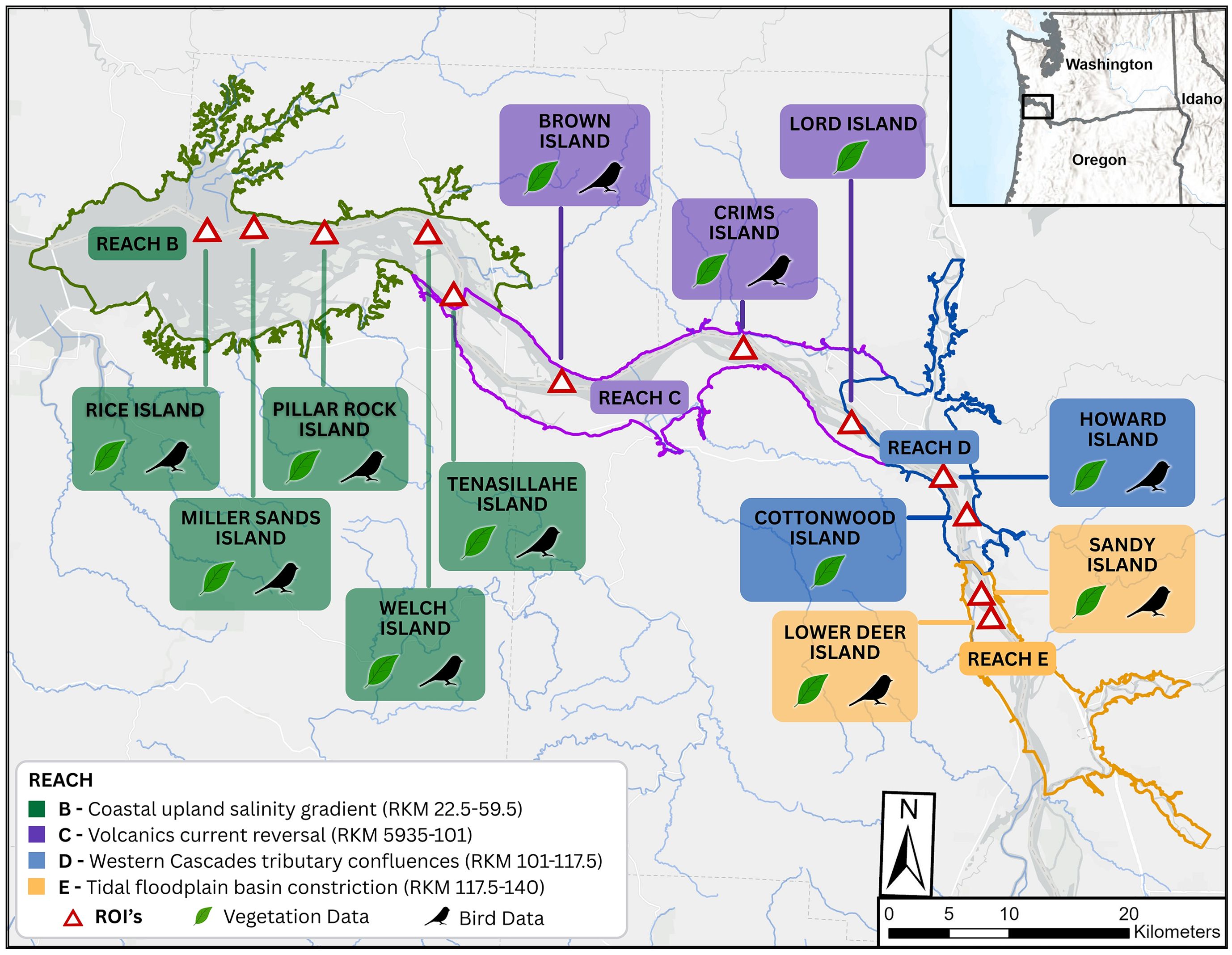
Figure 1. Study sites and hydrogeomorphic reaches within the Lower Columbia River study region. Study sites were defined spatially using region of interest (ROI) polygons detailed in the methods. Locations used in the models fit to NDVI trends over time by site are labelled with a leaf icon, while those fit to lark counts are marked with the bird’s black silhouette (methods discussed in sections 2.2 and 2.3, respectively). In section 2.4 we collected all NDVI values found at lark locations identified in the 2023 breeding season across all dredged deposit sites except for Sandy Island that had no larks that year.

Figure 1 illustrates the spatial extent of the LCR as addressed within this paper (rkm 22.5 to 140) and shows four of the river’s eight hydrogeomorphic reaches, extending laterally into the historical floodplain of the main river and its tidally influenced tributaries (Simenstad et al., 2011). Each of the four applicable reaches (B-E) display different attributes of river morphology, bedforms, tributary interaction, and hydraulic or tidal conditions that interact to drive flow and inundation patterns that impact the composition of ecological communities and their activity (Borde et al., 2020). Briefly, Reach B defines the inland extent of the salinity intrusion. It represents a convergence from open and peripheral bays into a confined fluvial valley with a mosaic of islands, shoals, and tidal channels. Reach C is confined to a valley that bisects the Coastal Range but still contains large, swampy mid-channel islands, tidal channels, sloughs, and flood plains. Tidal influence persists in this reach but slowly diminishes as one moves upstream. The river becomes mostly confined in Reach D by broad bottomlands whose narrow floodplains are dissected by tidal and backwater channels. Fluvial discharge dominates river hydraulics for much of the year. Tidal fluctuations have a minor influence (0.30 – 1.52 m) on the river’s hydraulics in Reach E, where the river becomes narrowly confined by bedrock valley sides and terrace deposits. Flood discharges here have produced prominent channel migration bar-and-swale morphology on the islands and floodplains, which themselves are thinly capped by fine sediments deposited from overbank flooding.

Figure 1 also illustrates the sites that were used in the analyses. The set of sites used varied a little when fitting models to the NDVI data (section 2.2) and the lark count data (section 2.3); these distinctions are noted in the figure and explained in the respective sections. When exploring lark-NDVI spatial associations explicitly, we relied on the most recently available breeding season’s data only (2023), which excluded Sandy Island because no larks were found that year. The set of sites used in these analyses all share similar dredge deposition approaches but can vary with respect to the amount of material placed, where it is placed, and how often. Given the sediment composition of the system, most dredge material is composed of sand and is either piped upland onto the islands, used to replace eroded shorelines or extend them, and in open water. For example, sites like Pillar Rock and Miller Sands Islands began with open water placements in the 1950’s. Placement activity then extended to beach nourishment and upland placements in the 1970’s to improve stability and continue to the present.

2.2 Regional changes in NDVI

2.2.1 Satellite imagery

We selected 12 historic dredged material placement sites along 179 rkm of the LCR for a targeted assessment of potential ecological benefits. Analyses were spatially confined to a region of interest (ROI), which is a polygon delineating each site’s study area. ROIs were defined using data from imagery and tabular records synthesized by Hatten et al. (2019). The ROIs used in this analysis were confined at each site to areas that had no record of receiving dredged material deposition for at least the last 30 years, which includes all sites depicted with a leaf in Figure 1. Satellite imagery was taken from the Landsat 7 data, which have a 30 m resolution (U.S. Geological Survey (USGS), 2025a). Images were gathered, filtered, and processed using Google Earth Engine (Gorelick et al., 2017). Below we review our reasoning and steps taken in additional detail. The code necessary to replicate these efforts is included in the Supplementary Material.

Within each site’s ROI we filtered and integrated all images from 1999–2023 to calculate NDVI values. NDVI is derived from the ratio of near-infrared (NIR) and red reflectance captured by satellite sensors and defined as NDVI = (NIR – RED)/(NIR + RED). NDVI values are continuous within a closed interval of [-1,1], whereby values can include the extremes of -1 and 1. NDVI values less than 0.1 are typically filtered out as non-vegetated (Pettorelli et al., 2005; Shen et al., 2015), but we retained small values, 0 < NDVI ≤ 0.1, to allow dry, non-vegetated areas to be included in this analysis. Shrubs and grasses result in values between 0.2 - 0.5, and values of 0.6 - 0.9 are found with the dense vegetation pattern typical of temperate or tropical forests (U.S. Geological Survey USGS, 2025b). Following convention, satellite images containing more than 10% cloud cover were filtered out, along with NDVI values less than 0 (NDVI ≤ 0 generally represent water and elevated moisture levels in the air from cloud cover that can increase measurement error; Justice et al., 2007; Shen et al., 2015; Hamel et al., 2009; Martinez and Labib, 2023). At each site, all available satellite images from each year were combined into a stack. This stack of images was then collapsed down to a single layer by retaining only the maximum recorded NDVI value per cell, providing a matrix of peak vegetative potential at the site within that year. Finally, we calculated the spatial mean of this peak growth across the site, thereby collapsing the matrix of maximum NDVI values to a single spatial average. The process was repeated across years at each site.

2.2.2 NDVI modeling

We fit a series of Bayesian generalized linear mixed models to the terrestrial NDVI data to test our hypothesis regarding whether levels of NDVI have changed over time and whether any observed changes varied across the river’s hydrogeomorphic zones. As previously stated, the maximum NDVI values observed at a given site were averaged over the ROI to provide a mean value per site per year. Note that while the values being modeled represent averages, we simply retain the NDVI abbreviation when referring to this metric to avoid confusion with predicted means. The filtering procedures described in section 2.2.1 further restricted the data to an open interval of (0,1), which excluded the endpoints of 0 or 1. These constraints reflect the NDVI values expected at our sites, but do not conform to the assumptions of a Normal distribution. To properly account for the nature of these data, we used generalized linear models with a Beta distribution as the likelihood function.

In addition to the limited range of values the data could exhibit, our sites were unevenly spread out across the reaches, the precise age of the sites was unknown beyond being 30+ years old, and we were interested in how these values changed over time. We therefore adopted a multi-level approach, also known as a mixed-model, to account for these obstacles by grouping the data by site. The use of generalized linear mixed-models can also result in improved parameter estimates when the data are expected to be more similar over time (temporal correlation) within a group than across them (Zuur et al., 2009). Sites were included as a random intercept, which helped account for repeated measures within sites and for the potential for additional variability in the initial conditions across sites, given the uncertainty in deposition age. We also explored whether allowing the slopes to vary by site improved the predictive performance of our models.

With the above considerations our null model was:

$\begin{array}{ll}{\text{NDVI}}_i\sim \text{Beta}({\text{μ}}_i,\varphi )& (1)\end{array}$

$\begin{array}{ll}\text{logit}({\text{μ}}_i)={\text{α}}_{\text{site}[i]}& (2)\end{array}$

$\begin{array}{ll}{\text{α}}_j\sim \text{Normal}(\overline{\text{α}},\text{σ})& (3)\end{array}$

$\begin{array}{ll}\overline{\text{α}}\sim \text{Normal}(-1.0,0.5)& (4)\end{array}$

$\begin{array}{ll}\text{σ}\sim \text{Exponential}(1.0)& (5)\end{array}$

$\begin{array}{ll}\varphi \sim \text{Gamma}(4.0,0.1)& (6)\end{array}$

where the distribution of each observation, NDVI_i, was expected to vary according to a Beta distribution with mean ${\mu }_i$ Equation 1 and concentration parameter $\varphi$. Equation 2 is our null model, M0, for the mean expected value, which is an intercept only regression in which the mean response is not expected to change based on any covariates. The ${\text{α}}_{\text{site}[i]},$ term reflects that the intercept varies by site for each observation i and represents our random intercept. Equation 3 states that for each of the j sites, the intercept is expected to vary according to a Normal distribution around a mean of $\overline{\text{α}}$ with variance $\text{σ}$. The hyperparameters $\overline{\text{α}}$ and $\text{σ}$ are themselves drawn from Normal and Exponential distributions, respectively. Values for the hyperparameters in Equations 4 and 5, along with the parameters for the Gamma distribution of $\varphi$ in Equation 6, represent skeptical priors based on expected associations between NDVI values and vegetation classes (Pettorelli et al., 2005; U.S. Geological Survey USGS, 2025b), and prior predictive simulations.

We then proceeded to fit a series of models to include the effect of time (years) and space (hydrogeomorphic reach) on the expected response, ${\mu }_i$. We fit two models to account for time:

$\begin{array}{ll}M1:\text{logit}({\mu }_i)={\alpha }_{\text{site}[i]}+{\beta }_1\text{yearS}& (7)\end{array}$

$\begin{array}{ll}M2:\text{ logit}({\text{μ}}_i)={\text{α}}_{\text{site}[i]}+{\text{β}}_{1,\text{site}[i]}\text{yearS}& (8)\end{array}$

where yearS is the range of years standardized to increase from 0 to 23. Beginning with model M2 in Equation 2 we allowed both the intercept and slope to vary by site to reflect the potential for sites to differ in both their initial NDVI levels and their rates of change over time. Importantly, the $\text{α}$ and $\text{β}$ parameters in models M2 onward covary, which enables us to identify additional structural dependencies between them. One example of interest is discerning how rates of change in primary productivity over time vary with the initial amount of productivity established. Lastly, spatial effects were implicitly included by encoding the hydrogeomorphic reach where sites were located and assuming that reach had an independent (M3, Equation 9) or interactive effect (M4, Equation 10) with time:

$\begin{array}{ll}M3:\text{ logit}({\text{μ}}_i)={\text{α}}_{\text{site}[i]}+{\text{β}}_{1,\text{site}[i]}{\text{yearS}}_{\text{i}}+{\text{β}}_2{\text{reach}}_i& (9)\end{array}$

$\begin{array}{ll}M4:\text{logit}({\mu }_i)={\alpha }_{\text{site}[i]}+{\beta }_{1,\text{site}[i]}{\text{yearS}}_i+{\beta }_2{\text{reach}}_i+{\beta }_3({\text{reach}}_i·year{S}_i)& (10)\end{array}$

Models were run using the Stan statistical platform (Stan Development Team, 2024) within the R software environment (version 4.42; R Core Team, 2024) under the brms package (Bürkner, 2017). All models were run with Hamiltonian Markov Chain Monte Carlo simulations using 4 chains for 10,000 iterations that each included 5,000 iterations as warm-up periods. Model convergence was based on a visual inspection of the chains and posterior predictive checks. These efforts were supplemented by verifying the effective sample size to ensure that enough independent samples were drawn from the posterior (McElreath, 2020) and the Gelman-Rubin convergence diagnostic, $\widehat{R}$ (Vehtari et al., 2021). Parameter significance was evaluated using 68% and 95% credible intervals (CI). Models were compared based on predictive accuracy using differences in the expected log predictive density ($\Delta$ELPD). Pareto smoothed importance sampling was also used to identify points that had outsized influence on the posterior distributions of each model. This technique identified several (two to four) influential points in both our preliminary model fits using non-informative (default) prior distributions and in our final models that used restrictive prior distributions. These points were subsequently linked to satellite images that had poor coverage, resulting in estimates that were heavily biased by missing data, and subsequently fell well outside yearly fluctuations (see Supplementary Figure S1 in the Supplemental Materials). These values were omitted from our final analyses. Inspection of autocorrelation trends in the parameters of our final models did show signs of autocorrelation in our slope parameters, which decayed rapidly to zero after three to four lags. As a precaution, we explored whether including an autoregressive-term using different lags (up to four) improved the performance of our top models – it did not (see Supplementary Table S1 in the Supplemental Materials for details). Lastly, the effective sample sizes of our final models were all greater than an order of magnitude beyond what would be considered sufficient to generate reliable estimates from the posterior distribution (Bürkner, 2017).

2.3 Regional changes in lark abundance

We performed two analyses regarding lark abundance (counts) and their spatial distributions. First, we evaluated the long-term spatial and temporal trends in lark counts across all reaches between 2004 and 2023 with generalized linear mixed-models, as in section 2.2 for NDVI. Next, we used satellite imagery to calculate lark-specific NDVI values based on 2023 lark survey data and evaluated how lark geospatial use explicitly varied across reaches and within dredged material sites, as further described under section 2.4. Below we detail data collection, processing, and analytical methods and attempt to highlight the differences between the regional analysis of NVDI above and these directed lark specific analyses.

2.3.1 Lark survey data

Since this species of lark (E. a. strigata) was listed as threatened in 2013, the U.S. Army Corps’ Portland District has been required to monitor its population in the LCR and attempt to place dredged material in a manner that supports the continued existence of this species (U.S. Fish and Wildlife Service (USFWS), 1998; Anderson, 2013). Available lark survey data also predate listing and provides a temporal dataset between 2004 and 2023 to investigate how trends in their abundance and habitat use might vary between dredged material locations. While sampling protocols evolved over time, the sampling period, baseline biotic parameters, and level of effort to survey larks has remained consistent across years (Pearson, 2003; Pearson and Hopey, 2005; Pearson et al., 2016). The surveys that began in 2004 were limited to sites in Reach B and Reach C, but efforts were expanded to include all dredged material placement sites when the species was listed as threatened. As a result, data in Reach B and C spanned from 2004-2023, data from Reach D from 2016-2023, and Reach E from 2014-2023. Surveys were conducted during peak breeding season (May to June) and report the number of birds observed through visual sightings and their locations, providing presence-only data. Multiple surveys were conducted at each site across the breeding season and annual abundance estimates represent the highest count for any one survey for that year. Annual lark surveys used in this analysis are labelled with a lark silhouetted in Figure 1 (N = 10).

2.3.2 Lark modeling

In contrast to the regional NDVI analysis, which was confined to historical deposition areas (≥ 30 years since last known deposition), lark occupancy and abundance surveys were collected across all areas established by dredged material placement and therefore not limited to historical deposition areas. We adopted the same modeling procedure used in the regional NDVI analysis to determine if lark counts changed over time and hydrogeomorphic reach, albeit that these counts, C_i, were assumed to follow a Poisson distribution with a log link (Equations 11, 12). The Poisson distribution is well suited to model count data (McElreath, 2020) and is preferred to transforming the counts themselves to conform to assumptions of normality (O’Hara and Kotze, 2010). Our lark null model, M0, was:

$\begin{array}{ll}{\text{C}}_{\text{i}}\sim \text{Poisson}({\text{λ}}_{\text{i}})& (11)\end{array}$

$\begin{array}{ll}\text{log}({\text{λ}}_i)={\text{α}}_{\text{site}[i]}& (12)\end{array}$

$\begin{array}{ll}{\text{α}}_j\sim \text{Normal}(\overline{\text{α}},\text{σ})& (13)\end{array}$

$\begin{array}{ll}\overline{\text{α}}\sim \text{Normal}(2.0,0.5)& (14)\end{array}$

$\begin{array}{ll}\text{σ}\sim \text{Exponential}(1.0)& (15)\end{array}$

where the hyperparameters in Equations 13–15 reflected skeptical priors based on predictive simulations guided by previous population surveys (Pearson and Altman, 2005; Pearson et al., 2016). Aside from the change in likelihood and link function, lark models M0-M4 followed the same structure as those adopted in the regional NDVI analyses. All models were run using the same system as the regional NDVI analyses and followed identical diagnostic and model evaluation procedures. There were again modest signs of temporal autocorrelation that dampened quickly, yet effective samples sizes were well above necessary levels and the inclusion of auto-regressive terms spanning several orders were not found to improve model predictive performance (see Supplementary Table S2 in the Supplemental Materials).

2.4 Lark-NDVI associations

2.4.1 Satellite imagery

Whereas the previous analyses used a series of statistical models to evaluate coarse-grained spatial and temporal patterns in our metrics, here we adopted a simpler qualitative analysis with finer spatial resolution that we limited to areas with lark presence data. We then linked each recorded lark position to a localized estimate of NDVI. We will refer to the resulting lark-specific values as NDVI_L to distinguish them from the spatially averaged NDVI values used in statistical analysis described in section 2.2. These NDVI_L values were then used to identify potential lark habitat across all monitoring areas within each reach. We used the same study sites as section 2.3, except Sandy Island in Reach E, which had no lark detections in 2023, and restricted our efforts to the 2023 lark survey data for tractability given the higher spatial resolution of the work.

Satellite imagery was extracted from the Sentinel-2 satellite using Google Earth Engine (Gorelick et al., 2017), and NDVI_L values were calculated for each 10 m² cell that had a recorded lark occupancy. We elected to use Sentinel-2 satellite imagery, which began data collection in 2015, as it has greater resolution (10 m²) than the Landsat imagery (30 m²). Data processing was identical to the regional NDVI study (see section 2.2.1) except that imagery was filtered to collections with less than 20% cloud cover instead of 10% because the increased spatial resolution, relative to the Landsat 7 data, compensated for average elevated condensation in the images. Post processing of satellite imagery with these restrictions resulted in a range of five to nine usable images per reach during the breeding season from May to June. Second, in contrast to the regional NDVI analysis, NDVI_L values less than zero were included because they have been linked to observed lark locations (Hatten et al., 2019).

2.4.2 Spatial associations

Linking observed lark positions to NDVI values and then using this information to define suitable lark habitat was done as follows. Satellite images of a given region are available periodically based on their orbits and may not overlap directly with a survey. To compensate for this disconnect we calculated NDVI values from all satellite images available during the breeding season for each bird’s location and recorded their average value over time, which defines NDVI_L. We then grouped these NDVI_L values by reach. Based on the findings of Hatten et al. (2019), we assumed that those NDVI_L recorded at observed lark locations reflected suitable lark habitat. However, rather than use the entire observed range of NDVI_L values to define suitable habitat, we adopted a more conservative estimate based on the observed mean and standard deviation. The reason for this is two-fold. We might expect some variability in vegetative growth at a location over the nesting season, with the true estimate of NDVI being greater than or less than the value present at the time of observation. A similar concern arises spatially because the estimated home range of these birds is far larger (approximately 14,000 m²; Slater and Treadwell, 2019) than the resolution of the Sentinel-2 imagery (≤10 m²). These birds tend to be found in patchy habitats with sparse vegetation (Pearson and Altman, 2005; Pearson and Hopey, 2005), so that each point observation could be either overestimating or underestimating the vegetative areas where the birds spend more time.

Count data at lark monitoring sites were collected across the entirety of the dredged material area, which could include both regions of historic (≥ 30 years old) and contemporary (< 30 years old) deposition. We therefore added a set of ROIs representing those regions where dredged material were < 30 years old. Together these two sets of ROIs captured each site’s monitoring area. The number of cells in each set of ROIs (e.g. ≥ 30 years old and < 30 years old) that fell within the defined range of suitable habitat were summed by reach and converted to square kilometers. Lastly, we applied the same process to all areas outside our ROIs within the boundaries of each hydrogeomorphic reach (shown in Figure 1) as an estimate of potential non-surveyed suitable lark habitat.

3 Results

3.1 Regional changes in NDVI

Figure 2A shows the overall changes in NDVI over time and across sites and reaches. Trends were generally positive across the system, varied across reaches, but not significantly, and displayed an interesting correlation between their rate of change and average peak production level. In Figure 2B we see the $\text{Δ}$ ELPD values for each of the 5 models explored, with the best model, M2, given a value of zero for comparison. The three best performing models (starting from the bottom of Figure 2B) each included both a random intercept and slope term. Figure 2C shows how the average rate of increase in NDVI from the simplest top model, M2, displayed a modest, significantly positive trend across sites (${\text{β}}_1= 0.009[0.001, 0.016] 95\% CI)$. While model M2 was the top ranked model, it is informative to contrast models M2 and M4 for inference since their predictive performances were equivalent. An examination of the ${\text{β}}_3$ coefficient for the interaction between yearS and reach in M4 shown in Figure 2D suggests that the strength in the overall trend in NDVI over time did tend to be stronger in the lower regions (Reach B and Reach C) than in the upper regions (Reach D and Reach E), where we saw little evidence of any significant change (relative to a ${\text{β}}_3=0$, indicated by the vertical dashed line).

Figure 2

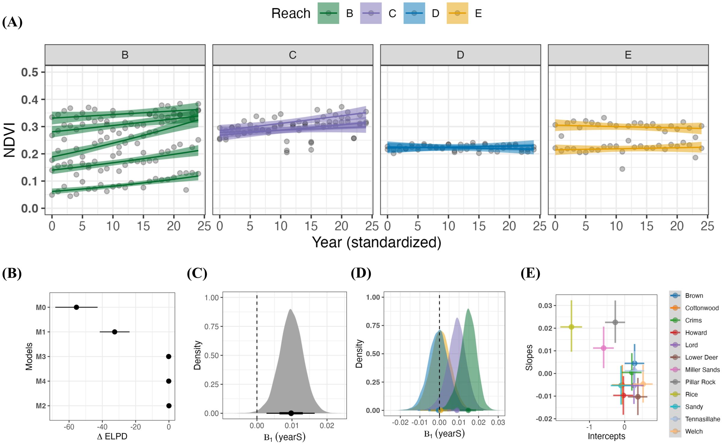
Figure 2. Spatio-temporal patterns in NDVI across a hydrogeomorphic gradient in the Lower Columbia River along the Oregon-Washington boundary from 2000-2023. (A) shows predicted trends and observed NDVI (points) across time by site and grouped by hydrogeomorphic reaches. Trends are from model M4 with 95% credible intervals and the raw data (grey points). (B) shows the mean model rankings (+/- 1 standard error) using differences in expected log-point density ($\text{ΔELPD}$) of each model with respect to the best performing model (M2). (C) shows the distribution of the slope parameter ${\text{β}}_1$ for time from model M2, along with a point estimate of its mean, 68% and 95% credible intervals. (D) shows how the same parameter in model M4 differs across reaches (yearS: reach interaction) using the interaction term from model M4. (E) shows the correlation between site-level estimates (mean) intercept and slope values (i.e., the random effects), taken from model M2, with their mean +/- 95% credible intervals. Median correlation value between the random intercept and slope terms was $\rho$ = -0.70.

One reason for using site as a random intercept in the models was due to uncertainty regarding the last known date of deposition within the 30+ year ROIs. Of the 12 sites investigated here, three displayed noticeably different initial conditions from the population average, Rice, Miller, and Welch Islands, which were all located in Reach B (see Supplementary Figure S2 in the Supplemental Material); suggesting that concerns over the impact of having varying deposition ages are likely limited to these few sites. An inspection of our varying levels (the ${\text{α}}_{\text{site}[i]}$ and ${\text{β}}_{1,\text{site}[i]}$ terms) also revealed a strong negative correlation between the initial productivity level and the rate of growth across sites, shown in Figure 2E. In this figure we can also see how Miller and Rice Islands have distinctly lower initial levels of NDVI and Welch Island has the highest.

3.2 Regional changes in lark abundance

Figure 3A shows differences in the average trends of lark abundance across sites and reaches. Counts remained constant or showed modest increases throughout the region, with some exceptions. The top model did not include reach as a predictor (M2) and the model comparisons shown in Figure 3B demonstrates that the $\text{ΔELPD}$ values did not support any predictive gain by the inclusion of reach in models M3 and M4. The net positive trend seen across the region (population average) shown in Figure 3C from model M2 was likely driven by the pronounced increase in larks observed at Rice Island, which can be seen exceeding 40 in the Reach B trends shown in panel A, along with the more modest gains at sites in Reach C. The remaining sites showed either modest increases (N = 3, Reaches B and C), stable patterns over time (N = 5; reaches B, D, and E) or a decrease (N = 1, Reach B). Abundance did tend to increase more in Reach B and Reach C, but panel (D) in Figure 3 shows how the pronounced overlap in slope values did not support a significant effect of reach.

Figure 3

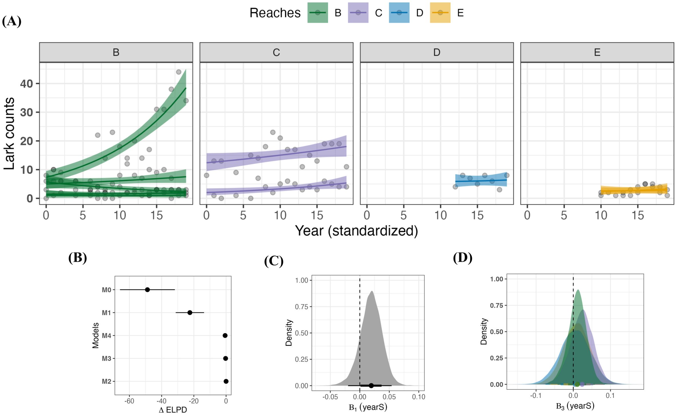
Figure 3. Spatio-temporal patterns in Streaked Horned Lark counts across the hydrogeomorphic gradient in the Lower Columbia River along the Oregon-Washington boundary. (A) shows lark counts across time by site, grouped by hydrogeomorphic reaches. Trends are from model M4 with 95% credible intervals and the raw data (grey points). Temporal coverage varied across reaches; Reach B and Reach C ranged from 2004-2023, Reach D from 2016-2023, and Reach E from 2014-2023. (B) shows the mean model rankings (+/- 1 standard error) using differences in expected log-point density ($\text{ΔELPD}$) of each model with respect to the best performing model (M2). (C) shows the distribution of parameter ${\text{β}}_1$ from model M2, along with a point estimate of its mean, 68% and 95% credible intervals. (D) shows how the slope varies by reach through the interaction term, ${\text{β}}_3$, using the interaction from model M4.

3.3 Lark-NDVI spatial associations

Figure 4 shows the distributions of lark-specific NDVI_L values across all reaches. These NDVI_L values had a global mean of 0.16 ± 0.13 (SD), which was subsequently used to define potential lark habitat (Table 1). These lark-specific NDVI_L values tended to increase in magnitude and variability as one moved downstream from reach E to B (Table 1; Figure 4). In Figure 5A we see that more potential lark habitat was found within the younger < 30-year-old areas, rather than in the older ≥ 30-year-old areas. An example illustrating the lark distributions by deposition age is shown in Figure 6 for Rice Island. Further, we observed a pattern of increasing placement area and more potential lark habitat than non-lark habitat downstream in reaches B and C. Lastly, Figure 5B shows that there was vastly more potential lark habitat across all reaches outside of the dredged material placement sites rather than in them. Collectively, we identified more (48.7 km²) potential lark habitat outside of dredged material areas versus within (3.1 km²) the dredged material placement areas evaluated in this study.

Figure 4

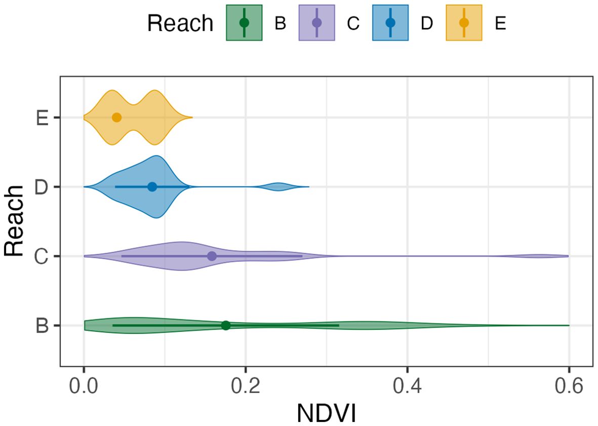
Figure 4. Distribution of NDVI_L measurements taken at lark locations in 2023 across reaches of interest in the lower Columbia River. Point and error bars represent the mean value ± 1 standard deviation that was then used to define lark suitable habitat by reach.

Table 1

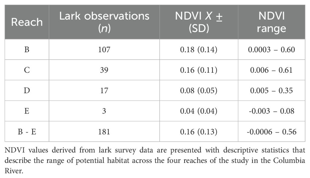
Table 1. Summary of 2023 Streaked Horned Lark NDVI habitat analysis.

Figure 5

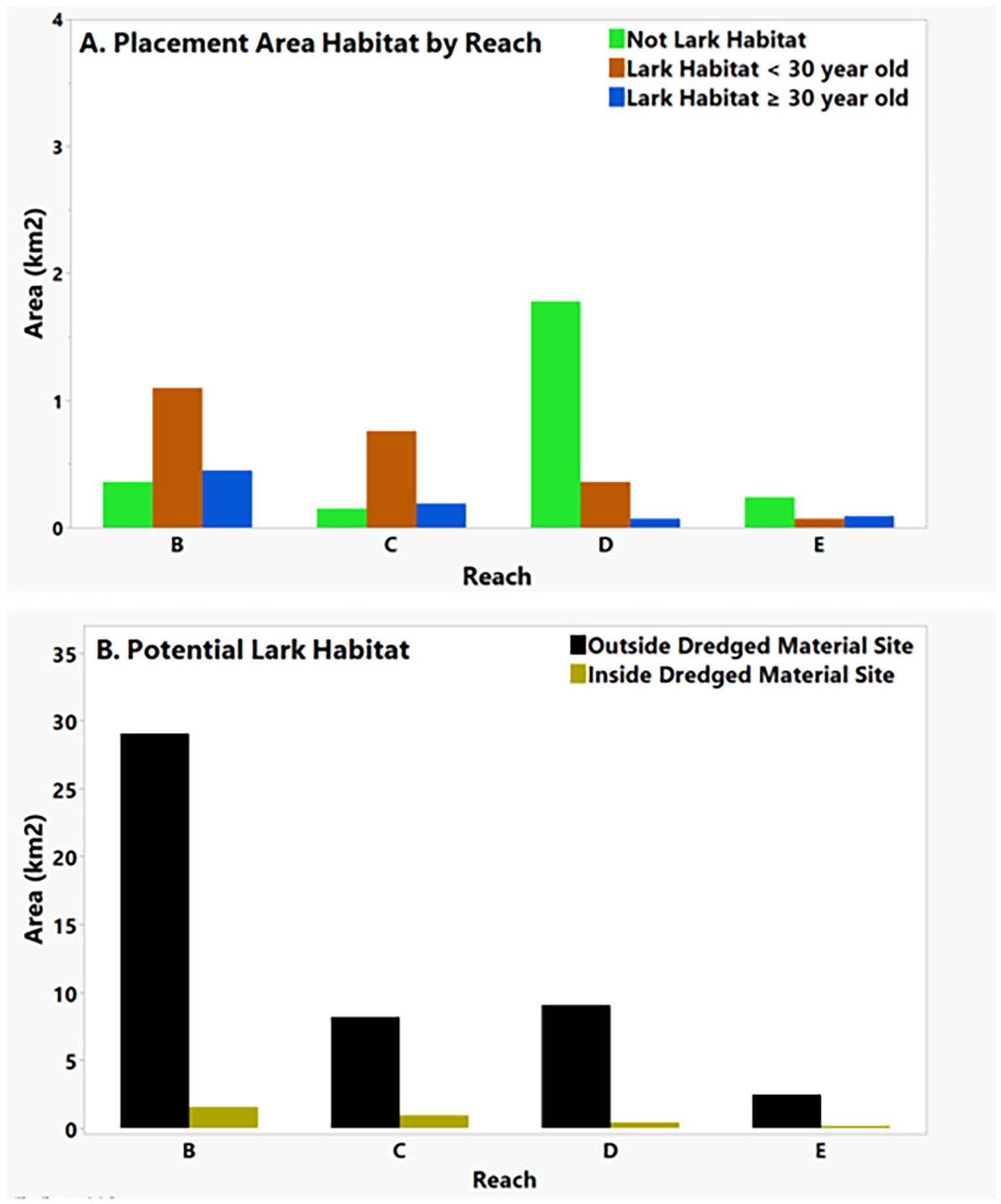
Figure 5. Area of dredged material sites and potential Streaked Horned Lark habitat based on NDVI measurements associated with 2023 lark detections in the lower Colombia River. (A) shows the distribution of potential lark habitat defined by NDVI values within 0.16 ± 0.13 (SD) on placement sites less than 30 years old (brown), greater or equal to 30 years old (blue), and the balance of the placement site that had NDVI values outside those measured for larks (green). (B) illustrates total potential lark habitat area identified outside (black) vs. inside (gold) the dredge material placement areas.

Figure 6

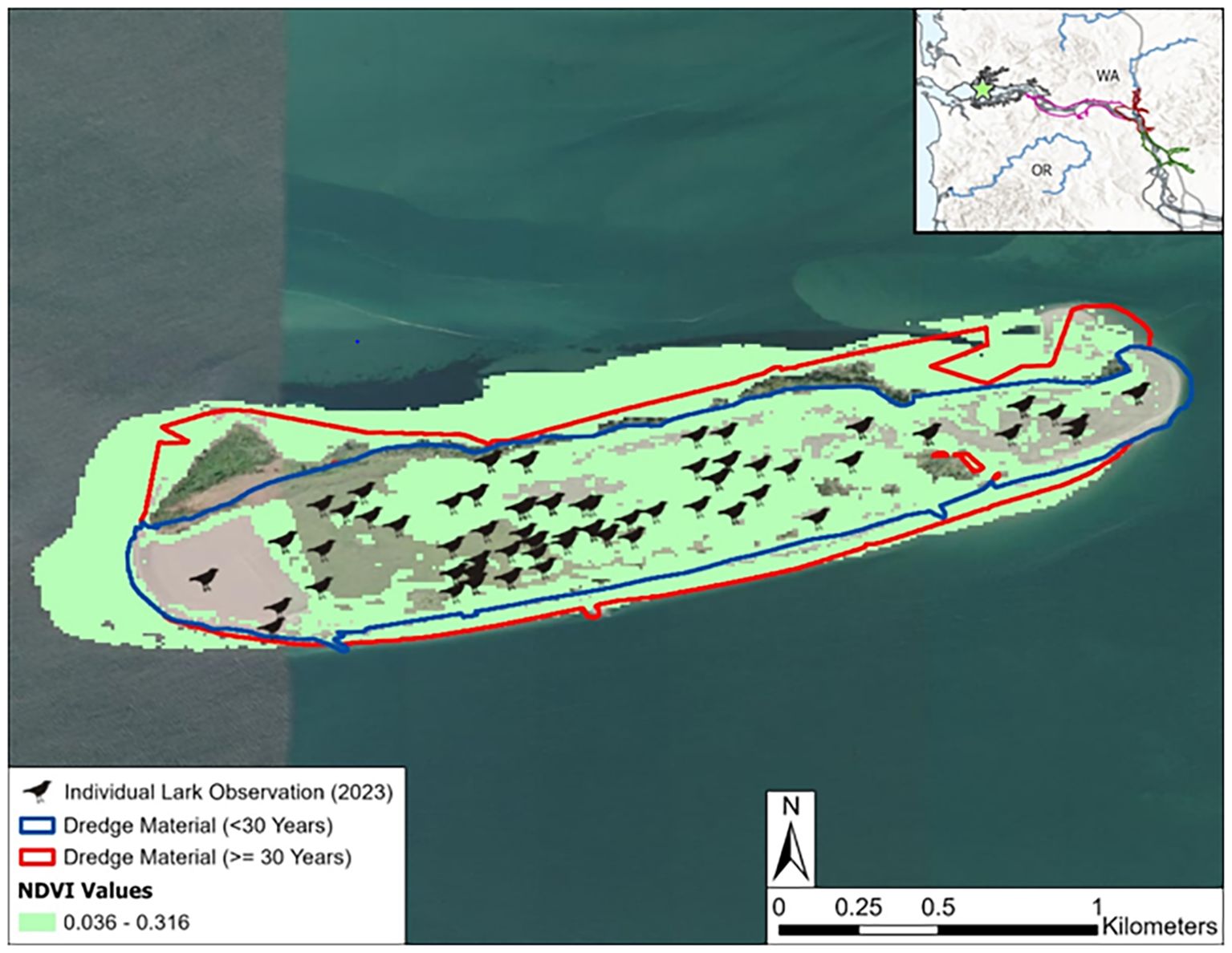
Figure 6. Streaked Horned Lark observations on Rice Island in 2023. Dredge material placement polygons are colored by time since last known deposition and lark locations are marked with icons. Potential habitat based on the suitable NDVI range derived from all lark observations is shared in green. The general location of the island is shown in the inset figure and can be seen in Figure 1.

4 Discussion

Habitat development is one of the primary goals for USACE BUDM projects (U.S. Army Corps of Engineers (USACE), 1987) to promote more economically, socially, and environmentally sustainable dredged material management approaches. A principal challenge of BUDM projects is that local objectives and constraints can vary across projects, yet we must balance these factors with the need to adopt a holistic view to advance the practice in general. There is also a need to help stakeholders relate to how ecological processes have evolved historically at dredged material placements within their region to inform community discussions. Here we used general statistical tools to quantify how two different ecological indicators have changed over time at dredged material placement sites. We used satellite-derived NDVI values and lark counts from monitoring data because they enabled us to adopt metrics that were locally meaningful, broadly relevant, and economic. Lark counts were an indicator requested by stakeholders, the use of NDVI values is easily transferable at the continental or global scale, and both approaches leveraged existing data that could be readily analyzed. While these efforts represent preliminary analyses, they could easily be expanded to help managers determine what to monitor and where and how to concentrate future efforts in a fiscally conservative fashion.

Our NDVI analysis revealed several insights, including a significant overall increase in vegetation across the portfolio, disentangled which reaches were driving that pattern, and identified an association between the rate of vegetative growth and the initial level of vegetation present. Overall, we detected a positive, albeit modest, degree of change in NDVI over time across dredge material sites throughout the study system. All averaged NDVI values were restricted to ranges representative of early successional flora, such as sedges, grasses, and shrubs. We did not find significant reach-level differences in NDVI across the hydrogeomorphic reaches, but sites in the lower Reaches B and C clearly drove the positive trend. Differences in the observed rates of change may be explained by differences in inundation patterns and vegetation community composition across the hydrogeomorphic reaches (Jay et al., 2016; Borde et al., 2020). Hydrogeomorphic reaches B and C used here, described by Simenstad et al. (2011), are characterized by tidally dominated zones that experience less overall inundation than the fluvially dominated zones located upstream.

Lacking detailed information of each site’s history was a concern that we addressed by including site as a random intercept in our models. Only Miller Sands, Welch, and Rice Islands showed notably different initial conditions from the remaining islands, with Rice and Miller Sands having some of the lowest initial NDVI values and Welch the highest. The remaining sites showed little differences in their initial conditions (see Supplementary Figures S1 and S2 in the Supplemental Material). Regarding the overall levels of NDVI observed, a variety of factors may have played a role, including community composition, successional stage, and underlying spatial heterogeneity. Recent analysis of the marsh-associated sections of Miller Sands and Welch Islands found a high proportion of invasive species (Borde et al., 2011), and observations during lark monitoring suggest that the presence of invasive species extends to the upland portions of the sites where European beachgrass (Ammophila arenaria) and scotch broom (Cytisus scoparius) are pervasive and seemingly dominant. Interestingly, Berkowitz et al. (2022a) found that the Miller Sands site displayed nearly equal levels of dominant species richness in the vegetation community between contemporary and historic levels. So, while species richness has changed very little, evidence suggests that community composition has shifted over time. Miller Sands had initially lower NDVI values that increased more rapidly over time than Welch Island, which had comparatively higher initial levels of NDVI that increased more slowly (Supplementary Figure S1 in the Supplemental Information). It is therefore more likely that successional stage or space availability had a greater impact on the average level and rate of change in NDVI at these locations than species composition. Given the correlation between initial NDVI levels and their rate of increase shown in Figure 2E, this pattern manifests across the portfolio. Linking the rate of growth between native and non-native flora using higher resolution imagery could enhance our ability to extract more ecological detail from this type of analysis and address the question of what role invasives play directly.

While our Bayesian analysis accounted for large-scale spatial effects at the reach level, it ignored the more granular effects at the site level because NDVI values were averaged across each site. Defining the ROIs to use was a primary challenge in this work because some areas were the result of sediment accretion from nearby depositions, and not from direct placement and thus fell outside of the ROIs. Sediment accretion patterns also tended to fluctuate over time. Most sites also contain a variety of habitats, including shoreline, recent emergent vegetation, and mature vegetation (e.g. shrubs and trees) on the upland dominated sections that was averaged over. Figure 6 illustrates how this summary statistic can obscure spatial variability in the case of Rice Island. The historic dredged material ROI contained peripheral areas devoid of much vegetation, while other locations contained shrubs and trees, e.g., the northern tip on the westward side of the island. Modeling relative changes in NDVI variability (e.g., by using the coefficient of variation) may provide additional insights across locations on how variation changes across projects. Nonetheless, while the spatial heterogeneity on display at Rice Island highlights the need for additional (spatial) resolution in evaluating ecological changes over time, the site’s overall performance still showed growth over time – underscoring the value of this initial assessment approach.

In contrast to the NDVI patterns, we found no significant increase in the average lark breeding population counts over time or any evidence of reach effects. This lack of significance is still informative, the trends are generally positive for efforts to protect the species, and certain sites suggest additional detail worthy of further investigation. Lark abundances were positive overall, with only one site showing a negative trend (Pillar Rock Island), another showing notable growth (Rice Island), three displaying modest increases (Miller Sands Island in Reach B, and Brown and Crims Islands in Reach C), and the remaining half of the sites were generally stable over time (see Figure 3A for site-level trends by reach; Supplementary Figure S3 in the Supplemental Materials for individual site-level trends). At a minimum, these trends suggest that the sites have provided reliable nesting grounds for this species over time. Most of the observed variation in counts at the majority of sites did not fluctuate beyond expectations (i.e., were within the 95% credible intervals of the trends). Adding more temporal structure did not improve the predictive value of the models, but there is clearly more complexity in some of the trends compared to the NDVI data. An exploration of placement activity at sights showing larger than expected fluctuations suggested that placement activities may have had less of an impact on the number of birds than where they were observed within sites. For example, Miller Sands and Brown Islands both showed stronger than average fluctuations around the expected counts over time. These birds predominantly nest in the upland regions at Miller Sands, yet there was no upland placement of dredged material there across the historical period evaluated (placements were done along the shoreline); a pattern suggesting that count fluctuations can occur without direct habitat impacts and may arise from sampling errors and demographic stochasticity alone. At Brown Island the observed count decreased after an upland placement event in 2014 but increased after a similar placement in 2019. This species is also both rare and cryptic, so it is difficult to interpret small fluctuations in survey counts across years. Upland placements of sand vary in location across each placement activity, resulting in a shifting mosaic of soil patches of different deposition age that may vary in vegetation patterns.

Locations with larks did not, on average, display pronounced levels of vegetation, i.e., NDVI. This is not unexpected because these birds prefer low vegetated areas (Pearson, 2003; Pearson and Altman, 2005; Pearson and Hopey, 2005), and many of these placement sites are actively managed to keep conditions favorable for the larks. Indeed, most of the lark habitat in the monitored areas were found in those less than 30 years old, which are also those areas that were disturbed more recently by dredged material placements. The site displaying the greatest increase in abundance over time was Rice Island; a site whose NDVI values over time showed only a modest increase from their relatively low initial conditions (see Supplementary Figure S1 in the Supplemental Material for NDVI growth rates by site). Due to habitat degradation throughout the Pacific Northwest, the lark’s range is believed to have been largely restricted to managed lands that provide disturbed soils with short, emergent vegetation that the birds prefer. The LCR dredged material islands used in this study support approximately 10% of the population and are a vital part of the lark’s range (Pearson and Altman, 2005). We identified almost 50 km² of NDVI-based potential habitat outside the dredge material placement areas and 0.8 km² of potential habitat within the ≥ 30-year-old placement areas that have not been extensively surveyed for larks. These new locations may warrant consideration for future surveys, given the assumption that most lark habitat is confined to managed lands (Pearson and Altman, 2005).

Even though this lark species displays a preference for the younger, less vegetated areas afforded by dredged material locations < 30 years old and displays higher abundance in reaches with more available area, there appears to be a limit to this tendency. For example, Reach C has more potential habitat than Reach D (Figure 5A) and more lark overall (Figure 3A), yet Reach D has more dredged material area – a pattern that draws the distinction between available area and potential (i.e., suitable) habitat. Dredged material placement occurs more frequently (almost every year) at the sites in Reach D than those in Reach C, resulting in a larger overall footprint that is perhaps less attractive habitat for this species due to the frequency of disturbance.

We note that the NDVI_L estimates used to define potential lark habitat in our study were, on average, greater than those reported by Hatten et al. (2019), but within one standard deviation of their reported estimates (their values: mean NDVI_L = 0.08 ± 0.09 [SD] and a range of -0.20 - 0.34). It is possible that our approach over-estimated the amount of potential habitat, but the effect is likely small given the overlap in average NDVI_L values observed at lark locations between our studies. The differences in mean observed values also does not indicate a biologically meaningful departure in expected vegetation levels (i.e., values < 0.2 tend to be sparsely vegetated; U.S. Geological Survey USGS, 2025b). Also, while presence-only data remain one of the most available for predicting species distribution patterns (Santini et al., 2021), these data neglect where species are not found and can introduce sampling biases that can influence spatial inference (Fithian et al., 2015). As such, approaches like the ones adopted here should be followed-up with more rigorous spatially-explicit methodologies to confirm observed trends beyond those observed at the dredged material placement sites.

Methodologically, the primary benefit of using multi-level models in these cases was that the models were able to offset uncertainty from data poor sites by ‘borrowing’ information from data rich sites to help inform population-level trends (i.e., by pooling information across groups). With a Bayesian approach, efforts can also provide informative priors to guide future work. Recent work demonstrated a similar benefit to improve model performance from rare species by borrowing prior parameter estimates from well-studied ones (Kindsvater et al., 2018). Such work could build on the current models by exploring causal connections between placement metrics, like area, frequency, or soil amendments (Liu et al., 2024), and then replacing the linear expectations (e.g., Equations 7-10) with predictive variables or a mechanistic function. With open access to satellite archives and the growth of tools to freely collate, preprocess, and analyze imagery data, documenting changes in biomass over large spatio-temporal scales has become a practical, economic, and biologically useful means of rapidly evaluating environmental impacts.

Efforts at locations in other regions may find themselves faced with similar constraints as presented here, where stakeholder concerns may be prioritized by species of either cultural or conservation concern. While addressing stakeholder needs is paramount to building consensus and promoting long-term support of restoration projects (Kumar et al., 2020), it will be imperative to also include one or more metrics that have broader significance, like changes in NDVI or other remote estimates of biomass. Future efforts could build on our approach to advance the practice by either testing if incorporating plantings or adding soil amendments to dredge material significantly increases changes in NDVI over time, or directing where to begin new population surveys for species of interest, as with the larks in our example. Leveraging data on the trends of ecologically salient indicators at existing or future BUDM sites can also help investigators develop hypotheses and avoid spurious tests, like assuming a null model of no vegetation growth at a site if you know a priori that your vegetation index previously showed growth over time (Popovic et al., 2024). Evaluating changes in emergent and subaquatic vegetation communities at BUDM sites could also complement NDVI results and provide a more holistic view of potential direct and indirect habitat benefits across a range of elevations. This is another area of potential investigation as remote sensing and drone technologies have enabled more robust datasets for submerged aquatic vegetation at both regional and national scales (e.g., Huber et al., 2021; Orth et al., 2022).

Challenges certainly remain, as increases in biomass at dredged material islands over time will not always translate to intended ecological outcomes. For example, in some regions dredged material islands provide needed sanctuaries for avian species (Harris et al., 2025), while in others the same process can be seen as a detriment if the avian species in question negatively impacts another species of concern (Collis et al., 2024). Further consideration may also be warranted for selecting the most relevant metric(s) for capturing the successional changes at BUDM sites over time, especially as many sites are actively managed for decades. Despite these hurdles, approaches like those taken here could help support BUDM practices nationally by providing data-driven insights to advance the practice and increase its transparency to our communities.

In conclusion, while there is evidence accumulating that demonstrates the potential ecological benefits from strategic placement of dredged material, trust in the process remains low among partner agencies and stakeholder groups. Long-term monitoring efforts and controlled field experiments can be costly barriers to implementing case studies, and there remains a need for practitioners to gravitate towards response metrics that are transferable across projects. We have presented case studies driven by stakeholder feedback to demonstrate how the use of readily available data can help overcome potential resource constraints, identify existing ecological trends, and guide future interventions.

Data availability statement

The original contributions presented in the study are publicly available. The data and code needed to replicate the results of this article are archived in the Zenodo repository under doi https://doi.org/10.5281/zenodo.17380499.

Author contributions

BL: Formal Analysis, Writing – original draft, Resources, Data curation, Conceptualization, Validation, Writing – review & editing, Investigation, Funding acquisition, Methodology. KT: Methodology, Data curation, Conceptualization, Investigation, Writing – review & editing, Validation, Formal Analysis, Writing – original draft. CJ: Methodology, Data curation, Conceptualization, Investigation, Validation, Writing – review & editing, Formal Analysis, Writing – original draft, Funding acquisition, Project administration, Resources. SC: Data curation, Writing – review & editing, Formal Analysis, Methodology, Validation, Visualization. HM: Writing – review & editing. ER: Writing – review & editing, Data curation, Investigation, Writing – original draft. MS: Writing – review & editing.

Funding

The author(s) declare financial support was received for the research and/or publication of this article. This work was funded and supported by the U.S. Army Corps of Engineers through the Coastal Resilience focus area of the Regional Sediment Management (RSM) Program.

Acknowledgments

The authors would like to acknowledge the U.S. Army Corps of Engineers RSM Program and staff for the continued support of this study as a phased approach to BUDM assessment. We also thank the USACE Portland District, Columbia Estuary Ecosystem Restoration Program for its continued contributions in Columbia River research efforts, and the Portland District Navigation Division and Operations Division Fisheries Field Unit for their continued efforts to monitor larks. Last, we acknowledge the contractors who collected the lark count and geospatial data over the years, Center for Natural Land Management and Turnstone Environmental. Special thanks to Gary Slater for providing historical lark distribution data and to Christopher Fincham for his help illustrating Figure 1.

Conflict of interest

The authors declare that the research was conducted in the absence of any commercial or financial relationships that could be construed as a potential conflict of interest.

Generative AI statement

The author(s) declare that no Generative AI was used in the creation of this manuscript.

Any alternative text (alt text) provided alongside figures in this article has been generated by Frontiers with the support of artificial intelligence and reasonable efforts have been made to ensure accuracy, including review by the authors wherever possible. If you identify any issues, please contact us.

Publisher’s note

All claims expressed in this article are solely those of the authors and do not necessarily represent those of their affiliated organizations, or those of the publisher, the editors and the reviewers. Any product that may be evaluated in this article, or claim that may be made by its manufacturer, is not guaranteed or endorsed by the publisher.

Supplementary material

The Supplementary Material for this article can be found online at: https://www.frontiersin.org/articles/10.3389/fevo.2025.1624170/full#supplementary-material

References

Abgrall C., Chauvat M., Langlois E., Hedde M., Mouillot D., Salmon S., et al. (2017). Shifts and linkages of functional diversity between above-and below-ground compartments along a flooding gradient. Funct. Ecol. 31, 350–360. doi: 10.1111/1365-2435.12718

Crossref Full Text | Google Scholar

Anderson H. E. (2013). Streaked Horned Lark habitat analysis and dredge material deposition recommendations for the Lower Columbia River. Final Report to U.S. Army Corps of Engineers (Olympia, WA: Center for Natural Lands Management).

Google Scholar

Atlas W. I., Ban N. C., Moore J. W., Tuohy A. M., Greening S., Reid A. J., et al. (2020). Indigenous systems of management for culturally and ecologically resilient pacific salmon (Oncorhynchus spp.) fisheries. Bioscience 71, 186–204. doi: 10.1093/biosci/biaa144

PubMed Abstract | Crossref Full Text | Google Scholar

Azerrad J. M. (2023). Periodic status review for the Columbian White-Tailed Deer (Olympia, Washington: Washington Department of Fish and Wildlife). Available online at: https://wdfw.wa.gov/sites/default/files/publications/02329/draft_wdfw02329.pdf (Accessed October 22, 2025).

Google Scholar

Barnas K. A., Katz S. L., Hamm D. E., Diaz M. C., and Jordan C. E. (2015). Is habitat restoration targeting relevant ecological needs for endangered species? Using Pacific Salmon as a case study. Ecosphere 6, 110. doi: 10.1890/ES14-00466.1

Crossref Full Text | Google Scholar

Berkowitz J. F., Beane N. R., Hurst N. R., Jung J. F., and Philley K. D. (2022a). A multi-decadal assessment of dredged sediment beneficial use projects part 1: ecological outcomes. WEDA. J. Dredging. 20, 50–71.

Google Scholar

Berkowitz J. F., Beane N. R., Hurst N. R., Philley K. D., and Jung J. F. (2022b). A multi-decadal assessment of dredged sediment beneficial use projects part 2: ecosystem functions, goods, and services. WEDA. J. Dredging. 20, 72–89.

Google Scholar

Bolam S. G. and Rees H. L. (2003). Minimizing impacts of maintenance dredged material disposal in the coastal environment: a habitat approach. Environ. Manage. 32, 171–188. doi: 10.1007/s00267-003-2998-2

PubMed Abstract | Crossref Full Text | Google Scholar

Borde A. B., Diefenderfer H. L., Cullinan V. I., Zimmerman S. A., and Thom R. M. (2020). Ecohydrology of wetland plant communities along an estuarine to tidal river gradient. Ecosphere 11, 30. doi: 10.1002/ecs2.3185

Crossref Full Text | Google Scholar

Borde A. B., Zimmerman S. A., Kaufmann R. M., Diefenderfer H. L., Sather N. K., and Thom R. M. (2011). Lower Columbia River and estuary restoration reference site study 2010 Final Report and Site Summaries. PNWD-4262 (Richland, WA: Lower Columbia River Estuary Partnership by Battelle – Pacific Northwest Division). Available online at: https://www.estuarypartnership.org/sites/default/files/resource_files/RSS_2010_Report_FINAL_submitted.pdf (Accessed 30 April 2025).

Google Scholar

Bürkner P. C. (2017). brms: An R package for Bayesian multilevel models using Stan. J. Stat. Software. 80, 1–28. doi: 10.18637/jss.v080.i01

Crossref Full Text | Google Scholar

Chase J. M. and Myers J. A. (2011). Disentangling the importance of ecological niches from stochastic processes across scales. Philos. Trans. R. Soc. B.: Biol. Sci. 366, 2351–2363. doi: 10.1098/rstb.2011.0063

PubMed Abstract | Crossref Full Text | Google Scholar

Collis K., Roby D. D., Evans A. F., Lawes T. J., and Lyons D. E. (2024). Caspian tern management to increase survival of juvenile salmonids in the columbia river basin: progress and adaptive management considerations. Fisheries 49, 71–84. doi: 10.1002/fsh.11012

Crossref Full Text | Google Scholar

Cura J. J., Bridges T. S., and McArdle M. E. (2004). Comparative risk assessment methods and their applicability to dredged material management decision-making. Hum. Ecol. Risk Assess. 10, 485–503. doi: 10.1080/10807030490452160

Crossref Full Text | Google Scholar

Dawe N. K., Bradfield G. E., Boyd W. S., Trethewey D. E. C., and Zolbrod A. N. (2000). Marsh creation in a northern Pacific estuary: Is thirteen years of monitoring vegetation dynamics enough? Conserv. Ecol. 4, 12. Available online at: http://www.consecol.org/vol4/iss2/art12/ (Accessed October 22, 2025).

Google Scholar

Diefenderfer H. L., Borde A. B., Cullinan V. I., Johnson L. L., and Roegner G. C. (2024). Effects of river infrastructure, dredged material placement, and altered hydrogeomorphic processes: The stress ecology of floodplain wetlands and associated fish communities. Sci. Total. Environ. 957, 176799. doi: 10.1016/j.scitotenv.2024.176799

PubMed Abstract | Crossref Full Text | Google Scholar

Diefenderfer H. L., Johnson G. E., Thom R. M., Borde A. B., Woodley C. M., Weitkamp L. A., et al. (2013). An evidence-based evaluation of the cumulative effects of tidal freshwater and estuarine ecosystem restoration on endangered juvenile salmon in the Columbia River. PNNL-23037. Final report prepared for the U.S. Army Corps of Engineers Portland District, Portland, Oregon (Richland, Washington: Pacific Northwest National Laboratory and NOAA Fisheries).

Google Scholar

Evans D. M., Che-Castaldo J. P., Crouse D., Davis F. W., Epanchin-Niell R., Flather C. H., et al. (2016). Species recovery in the United States: increasing the effectiveness of the Endangered Species Act. Issues Ecol. 20, 28. Available online at: https://esa.org/publications/issues/ (Accessed July 31, 2025).

Google Scholar

Fithian W., Elith J., Hastie T., and Keith D. A. (2015). Bias correction in species distribution models: pooling survey and collection data for multiple species. Methods Ecol. Evol. 6, 424–438. doi: 10.1111/2041-210X.12242

PubMed Abstract | Crossref Full Text | Google Scholar

Gorelick N., Hancher M., Dixon M., Ilyushchenko S., Thau D., and Moore R. (2017). Google Earth Engine: Planetary-scale geospatial analysis for everyone. Remote Sens. Environ. 202, 18–27. doi: 10.1016/j.rse.2017.06.031

Crossref Full Text | Google Scholar

Hamel S., Garel M., Festa-Bianchet M., Gaillard J. M., and Côté S. D. (2009). Spring Normalized Difference Vegetation Index (NDVI) predicts annual variation in timing of peak faecal crude protein in mountain ungulates. J. Appl. Ecol. 46, 582–589. doi: 10.1111/j.1365-2664.2009.01643.x

Crossref Full Text | Google Scholar

Harris B. D., Ostojic A., Tedesco L. P., VanDerSys K., Bailey S., Shawler J. L., et al. (2025). Wetland elevation change following beneficial use of dredged material nourishment. Front. Ecol. Evol. 13. doi: 10.3389/fevo.2025.1518759

Crossref Full Text | Google Scholar

Hatten J. R., Slater G. L., Treadwell J. L., and Stevenson M. R. (2019). A spatial model of streaked horned lark breeding habitat in the Columbia River, USA. Ecol. Model. 409, 108734. doi: 10.1016/j.ecolmodel.2019.108734

Crossref Full Text | Google Scholar

Hong G. H., Kim S. H., Suedel B. C., Clarke J. U., and Kim J. (2010). A decision-analysis approach for contaminated dredged material management in South Korea. Integrat. Environ. Assess. Manage. 6, 72–82. doi: 10.1897/IEAM_2009-033.1

PubMed Abstract | Crossref Full Text | Google Scholar

Hubbell D. W. and Glenn J. L. (1973). Distribution of radionuclides in bottom sediments of the Columbia River estuary (GPO, Washington, D.C: USGS Professional Paper 433-L).

Google Scholar

Huber S., Hansen L. B., Nielsen L. T., Rasmussen M. L., Sølvsteen J., Berglund J., et al. (2021). Novel approach to large-scale monitoring of submerged aquatic vegetation: A nationwide example from Sweden. Integrat. Environ. Assess. Manage. 18, 909–920. doi: 10.1002/ieam.4493

PubMed Abstract | Crossref Full Text | Google Scholar

Hurlbert A. H. and Haskell J. P. (2003). The effect of energy and seasonality on avian species richness and community composition. Am. Nat. 161, 83–97. doi: 10.1086/345459

PubMed Abstract | Crossref Full Text | Google Scholar

Jay D. A., Borde A. B., and Diefenderfer H. L. (2016). Tidal-fluvial and estuarine processes in the lower columbia river: II. Water level models, floodplain wetland inundation, and system zones. Estuaries. Coasts. 39, 1299–1324. doi: 10.1007/s12237-016-0082-4

Crossref Full Text | Google Scholar

Johnson G. E., Thom R. M., Whiting A. H., Sutherland G. B., Berquan T., Ebberts B. D., et al. (2003). An ecosystem-based approach to habitat restoration projects with emphasis on salmonids in the Columbia River Estuary. Final Report No. PNNL-14412 (Richland, WA (United States: Pacific Northwest National Laboratory).

Google Scholar

Justice C. O., Eck T. F., Tanré D., and Holben B. N. (2007). The effect of water vapour on the normalized difference vegetation index derived for the Sahelian region from NOAA AVHRR data. Int. J. Remote Sens. 12, 1165–1187. doi: 10.1080/01431169108929720

Crossref Full Text | Google Scholar

Kammerer J. C. (1990). “Largest rivers in the United States,” United States Geological Survey. Open file report 87-242 2pp. USGS, Virginia. Available online at: https://pubs.usgs.gov/of/1987/ofr87-242/ (Accessed April 30, 2025).

Google Scholar

Katz S. L., Barnas K., Hicks R., Cowen J., and Jenkinson R. (2007). Freshwater habitat restoration actions in the Pacific Northwest: a decade's investment in habitat improvement. Restor. Ecol. 15, 494–505. doi: 10.1111/j.1526-100X.2007.00245.x

Crossref Full Text | Google Scholar

Kindsvater H. K., Dulvy N. K., Horswill C., Juan-Jordá M.-J., Mangel M., and Matthiopoulos J. (2018). Overcoming the data crisis in biodiversity conservation. Trends Ecol. Evol. 33, 676–688. doi: 10.1016/j.tree.2018.06.004

PubMed Abstract | Crossref Full Text | Google Scholar

Kumar P., Debele S. E., Sahani J., Aragão L., Barisani F., Basu B., et al. (2020). Towards an operationalisation of nature-based solutions for natural hazards. Sci. Total. Environ. 731, 138855. doi: 10.1016/j.scitotenv.2020.138855

PubMed Abstract | Crossref Full Text | Google Scholar

Lake P. S. (2000). Disturbance, patchiness, and diversity in streams. J. North Am. Benthol. Soc. 19, 573–592. doi: 10.2307/1468118

Crossref Full Text | Google Scholar

Lee Y. W., Bogardi I., and Stansbury J. (1991). Fuzzy decision making in dredged-material management. J. Environ. Eng. 117, 614–630. doi: 10.1061/(ASCE)0733-9372(1991)117:5(614

Crossref Full Text | Google Scholar

Littles C. J., Trachtenbarg D. A., Moritz H. R., Swanson D. C., Woolbright R. W., Herzog K. M., et al. (2024). Site selection and conceptual designs for beneficial use of dredged material sites for habitat creation in the Lower Columbia River. ERDC/CHL TR-24-10 (Vicksburg, MS: US Army Engineer Research and Development Center), 41. doi: 10.21079/11681/48550

Crossref Full Text | Google Scholar

Liu J., Zhang T., Xu X., Xu J., Song S., Yang W., et al. (2024). Effects of different soil amendments on dredged sediment improvement and impact assessment on reed planting. Ecol. Eng. 206, 107306. doi: 10.1016/j.ecoleng.2024.107306

Crossref Full Text | Google Scholar

Martinez A. and Labib S. M. (2023). Demystifying normalized difference vegetation index (NDVI) for greenness exposure assessments and policy interventions in urban greening. Environ. Res. 220, 115155. doi: 10.1016/j.envres.2022.115155

PubMed Abstract | Crossref Full Text | Google Scholar

McElreath R. (2020). “Statistical rethinking,” in A Bayesian course with examples in R and Stan, 2nd Ed (CRC Press, Boca Raton, FL).

Google Scholar

Morhange C. and Marriner N. (2010). Mind the (stratigraphic) gap: Roman dredging in ancient Mediterranean harbours. Bollettino di Archeologia on line. Volume Speciale B / B7 / 4. Available online at: https://bollettinodiarcheologiaonline.beniculturali.it/portus-ostia-and-the-ports-of-the-roman-mediterranean-contributions-from-archaeology-and-history/ (Accessed 30 April, 2025).

Google Scholar

Nemani R. and Running S. (1997). Land cover characterization using multitemporal red, near-IR, and thermal-IR data from NOAA/AVHRR. Ecol. Appl. 7, 79–90. doi: 10.1890/1051-0761(1997)007[0079:LCCUMR]2.0.CO;2

Crossref Full Text | Google Scholar

O’Hara R. B. and Kotze D. J. (2010). Do not log-transform count data. Methods Ecol. Evol. 1, 118–122. doi: 10.1111/j.2041-210X.2010.00021.x

Crossref Full Text | Google Scholar

Orth R. J., Dennison W. C., Gurbisz C., Hannam M., Keisman J., Landry J. B., et al. (2022). Long-term annual aerial surveys of submersed aquatic vegetation (SAV) support science, management, and restoration. Estuaries. Coasts. 45, 1012–1027. doi: 10.1007/s12237-019-00651-w

Crossref Full Text | Google Scholar

Pearson S. F. (2003). Breeding phenology, nesting success, habitat selection, and census methods for the streaked horned lark in the Puget lowlands of Washington. Natural Areas Report 2003-02 (Olympia WA: Washington State Department of Natural Resources).

Google Scholar

Pearson S. F. and Altman B. (2005). Range-wide streaked horned lark (Eremophila alpestris strigata) assessment and preliminary conservation strategy (Olympia, WA: Washington Department of Fish and Wildlife), 25.

Google Scholar

Pearson S. F. and Hopey M. (2005). Streaked horned lark nest success, habitat selection, and habitat enhancement experiments for Puget lowlands, coastal Washington and Columbia River islands. Natural Areas Program Report 2005-1 (Olympia, WA: Washington Dept. of Natural Resources).

Google Scholar

Pearson S. F., Linders M., Keren I., Anderson H., Moore R., Slater G., et al. (2016). Survey protocols and Strategies for Assessing Streaked Horned Lark Site Occupancy Status, Population Abundance, and Trends (Washington Department of Fish and Wildlife, Olympia, WA: Wildlife Science Division), 25.

Google Scholar

Pettorelli N., Vik J. O., Mysterud A., Gaillard J.-M., Tucker C. J., and Stenseth N. C. (2005). Using the satellite-derived NDVI to assess ecological responses to environmental change. Trends Ecol. Evol. 20, 503–510. doi: 10.1016/j.tree.2005.05.011

PubMed Abstract | Crossref Full Text | Google Scholar

Popovic G., Mason T. J., Drobniak S. M., Marques T. A., Potts J., Joo R., et al. (2024). Four principles for improved statistical ecology. Methods Ecol. Evol. 15, 266–281. doi: 10.1111/2041-210X.14270

Crossref Full Text | Google Scholar

Raleigh R. F., Miller W. J., and Nelson P. C. (1986). Habitat suitability index models and instream flow suitability curves: Chinook salmon. U.S Fish and Wildlife Service. Biol. Rep. 82, 64.

Google Scholar

R Core Team (2024). A Language and Environment for Statistical Computing, version 4.4.2 (Vienna, Austria: R Foundation for Statistical Computing). Available online at: https://www.R-project.org/ (Accessed 8 April 2025).

Google Scholar

Roegner G. C. and Johnson G. E. (2023). Export of macroinvertebrate prey from tidal freshwater wetlands provides a significant energy subsidy for outmigrating juvenile salmon. PloS One 18, e0282655. doi: 10.1371/journal.pone.0282655

PubMed Abstract | Crossref Full Text | Google Scholar

Rosado E. Q. and Alexandre A. S. (2020). Validation of flood risk maps using open source optical and radar satellite imagery. Trans. GIS. 24, 1208–1226. doi: 10.1111/tgis.12637

Crossref Full Text | Google Scholar

Santini L., Benítez-López A., Maiorano L., Čengić M., and Huijbregts M. A. (2021). Assessing the reliability of species distribution projections in climate change research. Diversity Distrib. 27, 1035–1050. doi: 10.1111/ddi.13252

Crossref Full Text | Google Scholar

Sather N. K., Johnson G. E., Teel D. J., Storch A. J., Skalski J. R., and Cullinan V. I. (2016). Shallow tidal freshwater habitats of the Columbia River: spatial and temporal variability of fish communities and density, size, and genetic stock composition of juvenile Chinook salmon. Trans. Am. Fisheries. Soc. 145, 734–753. doi: 10.1080/00028487.2016.1150878

Crossref Full Text | Google Scholar

Shafer D. J. and Streever W. J. (2000). A comparison of 28 natural and dredged material salt marshes in Texas with an emphasis on geomorphological variables. Wetlands. Ecol. Manage. 8, 353–366. doi: 10.1023/A:1008491421739

Crossref Full Text | Google Scholar

Shen M., Piao S., Cong N., Zhang G., and Jassens I. A. (2015). Precipitation impacts on vegetation spring phenology on the Tibetan Plateau. Global Change Biol. 21, 3647–3656. doi: 10.1111/gcb.12961

PubMed Abstract | Crossref Full Text | Google Scholar

Simenstad C. A., Burke J. L., O'Connor J. E., Cannon C., Heatwole D. W., Ramirez M. F., et al. (2011). Columbia River estuary ecosystem classification—concept and application. US Geol. Survey., 2011–1228, 54. doi: 10.3133/ofr20111228

Crossref Full Text | Google Scholar

Slater G. L. and Treadwell J. (2019). Columbia River Streaked Horned Lark Surveys and Monitoring. Final Report to USACE (Olympia, WA: Center for Natural Land Management).

Google Scholar

Solanki P., Jain B., Hu X., and Sancheti G. (2023). A review of beneficial use and management of dredged material. Waste 1, 815–840. doi: 10.3390/waste1030048

Crossref Full Text | Google Scholar

Sommer T. R., Nobriga M. L., Harrell W. C., Batham W., and Kimmerer W. J. (2001). Floodplain rearing of juvenile chinook salmon: evidence of enhanced growth and survival. Can. J. Fisheries. Aquat. Sci. 58, 325–333. doi: 10.1139/f00-245

Crossref Full Text | Google Scholar

Stan Development Team (2024). Stan user’s guide, version 2.35 (Stan development team). Available online at: https://mc-stan.org/docs/stan-users-guide/index.html (Accessed 8 April, 2025).

Google Scholar

Staver L. W., Morris J. T., Cornwell J. C., Stevenson J. C., Nardin W., Hensel P., et al. (2024). Elevation changes in restored marshes at Poplar Island, Chesapeake Bay, MD: I. Trends and drivers of spatial variability. Estuaries. Coasts. 47, 1784–1798. doi: 10.1007/s12237-023-01319-2

Crossref Full Text | Google Scholar

Suedel B. C., McQueen A. D., Wilkens J. L., Saltus C. L., Bourne S. G., Gailani J. Z., et al. (2021). Beneficial use of dredged sediment as a sustainable practice for restoring coastal marsh habitat. Integrat. Environ. Assess. Manage. 18, 1162–1173. doi: 10.1002/ieam.4501

PubMed Abstract | Crossref Full Text | Google Scholar

Taddia Y., Pellegrinelli A., Corbau C., Franchi G., Staver L. W., Stevenson J. C., et al. (2021). High-resolution monitoring of tidal systems using UAV: A case study on poplar island, MD (USA). Remote Sens. 13, 1364. doi: 10.3390/rs13071364

Crossref Full Text | Google Scholar

Turner W., Spector S., Gardiner N., Fladeland M., Sterling E., and Steininger M. (2003). Remote sensing for biodiversity science and conservation. Trends Ecol. Evol. 18, 306–314. doi: 10.1016/S0169-5347(03)00070-3

Crossref Full Text | Google Scholar

U.S. Army Corps of Engineers (USACE) (1987). Beneficial Uses of Dredged Material. Engineer Manual, EM 1110-2-5026 (Washington D.C: U.S. Army Corps of Engineers). Available online at: https://budm.el.erdc.dren.mil/guidance/EM_1110-2-5026.pdf (Accessed 30 July 2025).

Google Scholar

U.S. Army Corps of Engineers (USACE) (2015). Dredging and dredge material management. Engineer Manual. EM 1110-2-5025 (Washington D.C: U.S. Army Corps of Engineers). Available online at: https://www.publications.usace.army.mil/USACE-Publications/Engineer-Manuals/u43544q/647265646765/ (Accessed 30 July 2025).

Google Scholar

U.S. Fish and Wildlife Service (USFWS) (1998). Final Endangered Species Consultation Handbook: Procedures for Conducting Consultation and Conference Activities Under Section 7 of the Endangered Species Act (U.S. Fish and Wildlife Service and National Marine Fisheries Service). https://www.fws.gov/sites/default/files/documents/endangered-species-consultation-handbook.pdf (Accessed October 22, 2025).

Google Scholar

U.S. Fish and Wildlife Service (USFWS) (2013). Endangered and threatened wildlife and plants: determination of endangered status for the Taylor’s checkerspot butterfly and threatened status for the streaked horned lark; final rule. Fed. Regist. 78, 61452–61503.

Google Scholar

U.S. Geological Survey (USGS) (2025a). USGS Landsat 7 Level 2, Collection 2, Tier 1. Available online at: https://developers.google.com/earth-engine/datasets/catalog/LANDSAT_LE07_C02_T1_L2 (Accessed 17 April 2025).

Google Scholar

U.S. Geological Survey USGS (2025b). Remote sensing phenology. Available online at: https://www.usgs.gov/special-topics/remote-sensing-phenology/science/ndvi-foundation-remote-sensing-phenology (Accessed 2 April 2025).

Google Scholar

Vehtari A., Gelman A., Simpson D., Carpenter B., and Bürkner P.-C. (2021). Rank-normalization, folding, and localization: an improved R^ for assessing convergence of MCMC (with discussion). Bayesian. Anal. 16, 667–718. doi: 10.1214/20-BA1221

Crossref Full Text | Google Scholar

Weitkamp L. A., Beckman B. R., Van Doornik D. M., Munguia A., Hunsicker M., and Journey M. (2022). Life in the fast lane: feeding and growth of juvenile steelhead and Chinook salmon in main-stem habitats of the Columbia River estuary. Trans. Am. Fisheries. Soc. 151, 587–610. doi: 10.1002/tafs.10376

Crossref Full Text | Google Scholar

Yates K. L., Bouchet P. J., Caley M. J., Mengersen K., Randin C. F., Parnell, et al. (2018). Outstanding challenges in the transferability of ecological models. Trends Ecol. Evol. 33, 790–802. doi: 10.1016/j.tree.2018.08.001

PubMed Abstract | Crossref Full Text | Google Scholar

Zu Ermgassen S. O. and Löfqvist S. (2024). Financing ecosystem restoration. Curr. Biol. 34, R412–R417. doi: 10.1016/j.cub.2024.02.031

PubMed Abstract | Crossref Full Text | Google Scholar

Zuur A. F., Ieno E. N., Walker N. J., Saveliev A. A., and Smith G. M. (2009). Mixed effects models and extensions in ecology with R Vol. 574 (New York: springer), 574.

Google Scholar