 Matthew Bennion1*†
 Ashley A. Rowden2,3†
 Bradley R. Moore4,5†
 Owen F. Anderson3†Jordi Tablada6†
 Shane W. Geange6†
 Fabrice Stephenson7†
- 1National Institute of Water and Atmospheric Research, Hamilton, New Zealand
- 2School of Biological Sciences, Victoria University Wellington, Wellington, New Zealand
- 3National Institute of Water and Atmospheric Research, Wellington, New Zealand
- 4National Institute of Water and Atmospheric Research, Nelson, New Zealand
- 5Commonwealth Scientific and Industrial Research Organization, Hobart, TAS, Australia
- 6Department of Conservation, Wellington, New Zealand
- 7School of Natural and Environmental Science, Newcastle University, Newcastle-upon-Tyne, United Kingdom
Introduction: Vulnerable Marine Ecosystems (VMEs) are characterized by species that are at heightened risk of destruction or removal by bottom fishing. In the high seas, Regional Fisheries Management Organizations (RFMOs) are required to implement measures to prevent Significant Adverse Impacts (SAIs) on VMEs. Impact assessments are routinely conducted to inform said measures. The spatial scale at which impact assessments are conducted has a considerable impact on results obtained, and therefore on management actions taken. Bioregions can provide an ecologically relevant scale for impact assessments; therefore, the aim of this study was to develop a VME-specific bioregionalization to inform management of SAIs on VMEs.
Methods: Occurrence records of VME indicator taxa and spatially explicit environmental variables were compiled. Gradient forest models were applied to estimate taxon compositional turnover, and a hierarchical classification approach was used to generate groups. Statistical approaches and visual assessment were used to inform the appropriate number of groups to represent VME bioregions.
Results: A 7-group VME-specific bioregionalization for the western part of the South Pacific Ocean is presented and described in detail including summary statistics and descriptions of the environmental conditions which characterize each bioregion. Two distinct spatial estimates of uncertainty are provided for use in spatial planning. Average bioregion area was 635,428 km2 (range: 6,111 to 1,913,667 km2), with the largest, Bioregion 5, accounting for 43% of the study area.
Discussion: The bioregionalization presented offers an opportunity to conduct impact assessments at an ecologically relevant scale, with specific reference to VMEs. While this approach was developed to help inform management of VMEs in the South Pacific, the approach used could be applied for the spatial management of biodiversity in other areas beyond national jurisdiction.
1 Introduction
Bioregions are large areas of relatively homogeneous environmental conditions (Woolley et al., 2019), that correspond to large-scale biodiversity patterns (Spalding et al., 2007). Bioregionalisation processes can be used to divide large geographic regions into environmentally and ecologically distinct sub-units referred to as bioregions (Dunstan et al., 2018). Bioregions infer connectivity, where it is assumed that there is greater connectivity within bioregions, than between them (Klanten et al., 2023). In this way, bioregional boundaries denote dispersal barriers (albeit porous). It is for these reasons, that bioregions are often considered ecologically relevant scales for conservation management, and why adequate representation of bioregions is an important consideration for spatial management planning (Stephenson et al., 2023; Klanten et al., 2023). For instance, protecting a sufficient proportion of all bioregions can help manage the uncertainty or lack of information associated with species distributions (Foster et al., 2017) and contribute to the preservation of the overall biodiversity of a given area of interest (Day et al., 2012).
Seafloor ecosystems in the deep sea can be biodiverse, productive, and yet in many cases are poorly understood in terms of ecology and distribution (Gros et al., 2022). Bottom fishing (e.g., bottom trawling and longlining) in the deep sea (typically between c. 200 m and 1,400 m water depths) can remove and deplete vulnerable species that are part of seafloor ecosystems (Clark et al., 2016). As such, the United Nations General Assembly (UNGA) has passed resolutions that require Regional Fishery Management Organizations/agreements (hereafter RFMOs) to prevent Significant Adverse Impacts (SAIs) on Vulnerable Marine Ecosystems (VMEs) (UNGA, 2006, 2009, 2011). VMEs are groups of species, communities, or habitats that are classified as vulnerable to acute or chronic disturbance based on the characteristics that they possess, such as uniqueness or rarity, functional significance, fragility, slow growth rates, late maturity, long-lived, low or unpredictable recruitment and structural complexity (FAO, 2009). SAIs are impacts that compromise VME structure or function, via (i) impairing the ability for affected populations to replace themselves; (ii) degrading long-term productivity; or (iii) causing a significant loss of species richness, habitat, or community types on more than a temporary basis (FAO, 2009). RFMOs have developed a range of VME indicator taxa to identify potential vulnerable marine ecosystems (e.g., Parker et al., 2009). VME indicator taxa are groups of species whose presence, abundance and health can provide valuable information about the conditions of marine ecosystems and the impacts of bottom contact fishing, and which can be readily identified in fishing by-catch (Parker and Bowden, 2010). VME indicator taxa are defined at various taxonomic levels, which differ between RFMOs. Examples include stony corals (Scleractinia), sponges (Porifera), and sea pens (Pennatulacea).
To mitigate the risk of SAIs on VMEs, various strategies have been implemented by RFMOs, including spatial management measures (SPRFMO, 2020). To support the development of spatial management measures, predictive models are often applied to map the distribution and abundance of VME indicator taxa and infer the likely distribution of VMEs (recent examples include Bridges et al., 2023; Stephenson et al., 2024a; Bennion et al., 2024a, 2024; Stephenson et al., 2021). The design of spatial management measures intended to reduce the risk of SAIs on VMEs are often informed by benthic impact assessments (Kaikkonen et al., 2024). The scale at which these assessments are conducted can have a significant impact on their results, and therefore on management options (Hewitt et al., 2024; Falco et al., 2022). For example, impact assessments can be conducted at spatial scales informed by management, ecological, physical, or impact/activity considerations. Any of these scales may be appropriate, depending on feasibility and the needs of policymakers and environmental managers. For example, ecologically-based large spatial scales can be the most appropriate for managing broad, ecosystem-level impacts (for example regional fishery impacts and climate change impacts on VMEs), given they can describe scales relevant for connectivity; i.e., reflecting limits in larval dispersal attributable to the circulation of water masses (Ramiro-Sánchez et al., 2023). Different spatial scales can complement each other in impact assessments, where effective ecosystem-based management necessitates a multi-scale approach to ensure all relevant spatial scale components are considered (Guarinello et al., 2010; Hewitt et al., 2024).
Bioregions provide a framework for assessing impacts on large ecological scales, ensuring that assessments consider the natural boundaries and ecological characteristics of an area (Woolley et al., 2019). By using bioregions, impact assessments can better account for habitat suitability and connectivity, which are crucial for the survival of species with similar life histories and environmental responses (Elith and Leathwick, 2009). Incorporating bioregional information into impact assessments helps in identifying critical habitats and planning conservation efforts more effectively (Stephenson et al., 2023), including the design of effective marine protected areas (MPAs) (Grorud-Colvert et al., 2021). That is, adequate protection of each bioregion to ensure they can sustain their unique resident communities e.g., in terms of physical habitat and larval supply (Klanten et al., 2023). Additionally, for MPA network design, adequate protection of each bioregion across the network is deemed necessary to support representativity across the network (Robinson et al., 2017; Roberts et al., 2018; Brito-Morales et al., 2022).
Various bioregionalizations have been developed that either include, or are focused on, the seafloor ecosystems of the South Pacific Ocean (Beger et al., 2020). For example, Spalding et al. (2007) produced global ecoregions with provinces such as ‘Temperate Australasia’ and ‘Southern Ocean’. Costello et al. (2017) also produced global bioregions (~7 bioregions cover the western portion of the South Pacific Ocean where this study takes place) using a variety of biodiversity data, while Summers and Watling (2021) on the other hand, produced bioregions for octocorals in the Pacific Ocean. At more regional scales, Dunstan et al. (2018) used species distribution models as well as expert input and environmental characteristics to generate bioregions for the South West Pacific, while Beger et al. (2020) produced national-scale deep-water and reef-associated bioregions for Pacific Island nations using species distribution models. Stephenson et al. (2023) also produced a national- scale seafloor bioregionalization for the New Zealand Territorial Sea and Exclusive Economic Zone (EEZ) using a large dataset on benthic taxa. These bioregionalizations represent a variety of biological and ecological scales depending on the data available, the management applications, and wants and uses of end-users. In the South Pacific high seas, where the South Pacific Regional Fisheries Management Organization (SPRFMO) aims to manage sustainable bottom fisheries, a bioregionalization for VME indicator taxa can provide an appropriate ecological scale for designing and/or assessing spatial management measures to prevent and evaluate SAIs on VMEs. The aforementioned bioregions were deemed unsuitable for the area managed by SPRFMO, not only because they were not created solely with information on VME indicator taxa distribution, but in some cases, study extents did not overlap with the SPRFMO management area, or those that did, were deemed too coarse to be useful for management needs e.g., Costello et al. (2017).
The overall aim of our study was to develop a bioregionalization that could be used to inform the management of VMEs in the SPRFMO Convention Area (Bennion et al., 2024b). Accordingly, the main objectives of our study were to: 1) develop a spatially explicit estimate of VME indicator taxa compositional turnover in the South Pacific Ocean, 2) generate a bioregionalization for VME indicator taxa in this region, and 3) use biological and environmental data to describe the bioregionalization.
There are three main statistical approaches for developing bioregionalizations (Woolley et al., 2019; Ferrier and Guisan, 2006) (noting there are other approaches that use expert opinion, see UNESCO (2009)). These are: 1) approaches that group species data first, then spatially predict, or 2) the reverse, where species data is used to predict distribution and grouped in a second step (Woolley et al., 2019), and 3) approaches that do both steps simultaneously (Hill et al., 2017). For this study, we used an adapted version of approach 2 (‘predict first, then group’) given the flexibility afforded to the grouping stage after modelling i.e., it is possible to produce finer or coarser classifications post-hoc. To achieve our objectives, we used occurrence datasets of VME indicator taxa, environmental datasets, and Gradient Forest modelling (Ellis et al., 2012; Pitcher et al., 2011) to estimate taxon compositional turnover. We followed methods applied to demersal fish (Stephenson et al., 2018), seafloor invertebrate and macroalgae taxa (Stephenson et al., 2022) in New Zealand waters, and subsequent work to develop a hierarchical classification and bioregionalization (Stephenson et al., 2020b, 2023). Ideally, bioregions should be developed with regionally-specific biological information, as argued by Beger et al. (2020), given that spatially dynamic environmental regimes (e.g., in the South Pacific) likely drive biodiversity patterns at smaller scales than that of ocean basins typically recorded by global bioregionalizations. In this study, the use of occurrence information for VME indicator taxa within the study area only, means that classification and bioregionalizations are both regionally- and VME-specific.
2 Methods
To generate a bioregionalization for VME indicator taxa for the South Pacific Ocean, data of VME indicator taxa presence was used alongside environmental data, to model compositional turnover. A clustering approach was then used to generate a VME community classification, which was subsequently reduced to a bioregionalization (workflow shown in Supplementary Materials, Supplementary Figure S1). The approach used here is described in Bennion et al. (2024b) and follows closely the methods described by Stephenson et al. (2022) using Gradient Forest modelling, and Stephenson et al. (2023) for reducing a seafloor community classification to a bioregionalization. The study area used here matches Stephenson et al. (2021) and Bennion et al. (2024a) and includes depths of 200–3000 m in the western portion of the SPRFMO Convention Area (hereafter ‘SPRFMO Evaluated Area’), and the EEZs of various Pacific nations, primarily New Zealand (Figure 1). This area is relevant for SPRFMO management needs (encompassing the current ‘maximum fishable depth’ of 1400 m; SPRFMO, 2023), but also constitutes an area where high-resolution (1 km x 1 km) environmental data were available and the depth range represented the approximate combined bathymetric range of VME indicator taxa (Stephenson et al., 2021).
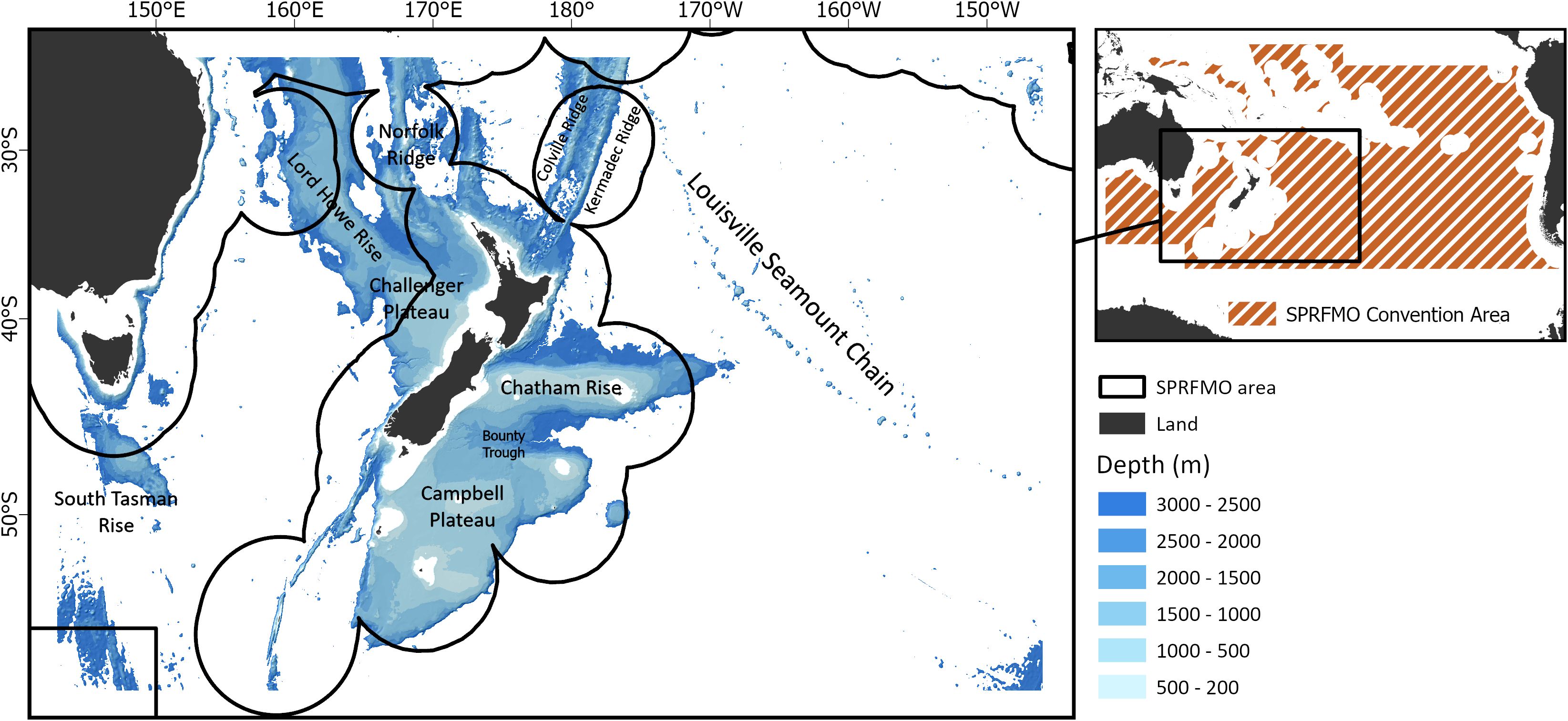
Figure 1. Map of water depth (bathymetry) across the study area (200 m to 3,000 m). Black lines indicate the boundaries between the western portion of the South Pacific Regional Fisheries Management Organisation (SPRFMO) Convention Area (i.e., SPRFMO Evaluated Area, shown via extent indicator) and Exclusive Economic Zones of various South Pacific nations. Labels indicate the broad area where large underwater topographic features are located.
2.1 Biological data
Occurrence (presence-only) data for VME indicator taxa used to train the Gradient Forest (GF) models were available from previous data compilation exercises (Geange et al., 2020) and habitat suitability modelling (Stephenson et al., 2021; Bennion et al., 2024a). These data are from New Zealand and Australian museum/collection records, fisheries research databases, and online biodiversity databases. Records were filtered to depths between 200–3000 m within the SPRFMO Evaluated Area, as per Stephenson et al. (2021) and Bennion et al. (2024a), and shown in Figure 1. The data were refined by checking for positional errors, verifying recorded depths against the most accurate bathymetry estimates for the region (Mackay et al., 2015), eliminating duplicate entries, and removing records outside the study area and 200–3000 m depth range. Presence records were spatially aggregated to a 1 km x 1 km grid resolution, i.e., a taxon was considered present in a given 1 km2 cell if there was any presence record from within that cell.
Unique labels of sampling gear/methods in the dataset were manually assessed. All records collected with gear/methods that were static or highly selective (e.g., grabs and pots) were omitted while methods recorded as mobile gear (trawl, dredge, and towed video) were kept (i.e., those gears that provide a sample commensurate with a 1 km x 1 km grid cell). Taxonomic information was extracted and compared to the World Register of Marine Species (www.marinespecies.org) to check and, where necessary, correct nomenclature (Chamberlain and Vanhoorne, 2023). Although VME indicator taxa recognized by SPRFMO cover several higher taxonomic levels [e.g., Phylum Bryozoa, Class Hydrozoa, and Order Zoantharia (SPRFMO, 2023)] we used finer taxonomic resolution data (i.e., genus level) as this was considered to produce more accurate compositional turnover functions using Gradient Forest models (see Gradient Forest modelling below). Otherwise, environmental gradients could be heavily influenced by taxa that are simply more highly represented in the occurrence dataset. Additionally, aggregating records to genus level provided a greater number of unique locations than when records were aggregated to species level. Where possible, all genus level records for VME indicator taxa were retained, but records with missing or erroneous taxonomic information for the genus level were removed. Following taxonomic filtering, and filtering to remove those instances of <10 unique location occurrences per genus (Stephenson et al., 2022), 182 genera were available for modelling. Following removal of non-modelled taxon presences, an occurrence matrix (presence-absence) with 3,341 unique locations remained (7,205 instances of taxon presence), for 182 genera of VME indicator taxa (Supplementary Figure S2). The number of genera per VME indicator taxon group was variable, with many times more Bryozoa genera (n = 59) included than Zoantharia genera (n = 1), for example (Table 1) noting that this imbalance is accounted for in the GF modelling approach (Ellis et al., 2012).
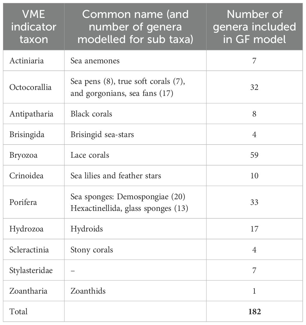
Table 1. Taxon groups modelled and the number of genera included in Gradient Forest (GF) models.
To estimate compositional turnover, GF models require an occurrence matrix of locations with presence-absence information. Similar to Stephenson et al. (2022), systematically collected absence records were not widely available across the study area or consistently available across sampling methods, an issue that is common in datasets from deep ocean environments (Ramiro-Sánchez et al., 2023). Instead, where a taxon has not been recorded at the same site as another, it is assumed to be absent from that location. This method is similar to the use of “target-group background” data (Phillips et al., 2009) in species distribution modelling where grid cells for which any of the taxa not being modelled are recorded as present, are assumed to represent absences for the target taxon (Stephenson et al., 2021). Previous GF models produced for the New Zealand EEZ generated separate models for ‘catchability’ classes based on sampling gear (Stephenson et al., 2022). This approach was explored here, but there were too few data to develop separate gear class GF models in this manner. Instead, it is assumed that by retaining only data sampled using mobile gears, different catchabilities are managed as best as possible given the data available at present.
2.2 Environmental data
The predictor variables (environmental datasets) used in the GF models here, are the same as those previously used to generate habitat suitability models for VME indicator taxa by Stephenson et al. (2021) and Bennion et al. (2024a), with the addition of depth and salinity from Georgian et al. (2019). However, while previous modelling efforts made use of substrate variables (percent mud and gravel), these were removed from model development in the testing phase due to artifacts noticed in spatial predictions attributable to the considerable interpolation required to build these layers. Although not directly comparable to the final model (due to differing settings and variables used), initial model runs including the substrate variables gravel and mud did not indicate extremely high relative importance (5th and 7th highest relative importance, respectively). The final set of environmental data comprised a combination of variables representing seafloor substrate proxies, water chemistry, and productivity; bathymetric position index-broad (BPI-Broad), standard deviation of slope (slope SD), ruggedness, dissolved oxygen at depth, aragonite saturation state at depth, temperature at depth, particulate organic carbon export to the seafloor (POC), depth, salinity, and silicate concentration (Supplementary Table S1).
2.3 Gradient Forest modelling
GF models (Ellis et al., 2012; Pitcher et al., 2011) make use of species distribution data (presence-absence or abundance) to manage the selection, weighting, and transformation of environmental predictors, aiming to maximize their correlation with changes in taxa composition and identify the points along environmental gradients where significant compositional shifts take place (Ellis et al., 2012). Transformed environmental variables, which represent species compositional turnover, can subsequently be classified to define spatial groups that reflect variations in taxa composition and turnover (Pitcher et al., 2011) either at finer-scale representing communities or broader-scales representing bioregions. For instance, within New Zealand’s EEZ, a combination of GF models have been used with occurrence information for macroalgae, demersal and reef fish, and seafloor invertebrates to generate the New Zealand Seafloor Community Classification or NZSCC (Stephenson et al., 2022). By reducing the level of classification detail of the NZSCC hierarchical classification (75 classes reduced to 9 groups), the Seafloor Bioregionalization for New Zealand was created (Stephenson et al., 2023). GF is an extension of the Random Forest (RF; Breiman, 2001) method, where the tree-split values from the RF models for all taxon models with positive fits (R2f > 0) are combined to generate empirical distributions which represent compositional turnover across environmental gradients (Ellis et al., 2012; Pitcher et al., 2011). The turnover function is quantified in dimensionless R2 units, with taxa that have high predictive power (high R2f values) exerting more influence on the turnover functions than those with lower predictive power (lower R2f). By using dimensionless R2 to measure species compositional turnover, data from multiple taxa can be integrated, even when that data comes from different sampling methods, surveys, or regions (Ellis et al., 2012). The dimensionless R2 used in GF models should not be confused with the commonly used coefficient of determination, also referred to as R2.
GF models were applied using the R package gradientforest (Ellis et al., 2012) and follow closely the methods detailed in Pitcher et al. (2011) and Stephenson et al. (2022). The GF models were trained using 250 trees, with the default correlation threshold of 0.5 applied in the conditional importance calculation of environmental variables. The GF model was bootstrapped (100 times), meaning that transformed environmental variables are a mean value across said bootstraps. An uncertainty estimate was produced at the same time (standard deviation, SD). The bootstrapping process involved generating GF models for the 182 genera 100 times, with randomly sampled sites (with replacement) equal in number to the total number of sites (i.e., 3,341).
The compositional turnover functions for each genus (shapes of the turnover curves) were used to transform the gridded environmental layers (1 km x 1 km grid), creating a “transformed environmental space” representing compositional turnover (Ellis et al., 2012; Pitcher et al., 2011). From the 100 bootstrapped iterations, transformed environmental layers were used to produce mean compositional turnover. Compositional turnover was visualized through Principal Components Analysis (PCA) and mapping, employing the same color scheme in the geographic representation of compositional turnover as used in the PCA plot (Pitcher et al., 2011). Compositional turnover was then used to produce biotic groups via hierarchical clustering (Stephenson et al., 2022; Leathwick et al., 2011). Clustering in a hierarchical manner means that if clustering is carried out for e.g., 50 groups, but bioregions are selected at a <10 group level, the higher-level groups (i.e., VME community groups) are nested within the delineated bioregions. The mean spatial estimate of compositional turnover from the GF model (i.e., the bootstrapped GF model) was classified using a two-stage approach (Stephenson et al., 2020b) using the R package cluster (Maechler, 2019). In the first stage, mean spatial estimates of compositional turnover were clustered to form 50 initial biotic groups using non-hierarchical, k-medoids clustering. For the second stage, a hierarchical clustering approach was employed via a flexible unweighted pair group method with arithmetic mean (UPGMA) using the Manhattan distance metric (Stephenson et al., 2022, 2018). This second classification step was undertaken at various levels of classification detail ranging from 3 to 50-group levels at increments of 1.
Following Snelder et al. (2007), Analysis of Similarities (ANOSIM) was used to assess the within- and between-group variation depending on classification detail. ANOSIM was implemented using the vegan package in R (Oksanen et al., 2013). The ANOSIM R value indicates whether the difference between groups (i.e., classes) is larger than within groups. Typically, low ANOSIM R values with fewer groups would be expected, as this means the variability within groups is larger than between them, with ANOSIM R increasing with increasing classification detail. The ‘optimal’ number of classes or groups for a bioregionalization depends on a variety of factors, but ANOSIM can assist with this choice (see Delineating the bioregions below) by providing descriptive support. Occurrence information (the biological training data) was tagged with classification detail, whereby each occurrence record was matched to the corresponding classification group at the given point location (this was repeated for 3 to 50-class group levels at increments of 1). The ANOSIM R-value was then used to assess differences between class groups. To supplement the results obtained from the ANOSIM approach, cluster quality indices (average silhouette width and Calinski–Harabasz) were also calculated using the cluster and fcp packages (Maechler, 2019; Hennig, 2019) in R. In contrast to the ANOSIM approach, these indices were calculated using the compositional turnover (20,000 random samples).
2.4 Environmental coverage
For management applications, it is important to fully acknowledge, and where possible, account for, uncertainty in models (Moilanen et al., 2006). Therefore, alongside the uncertainty estimates of compositional turnover (SD), a second spatially explicit estimate of uncertainty was created, referred to as environmental coverage (Supplementary Figure S1). Environmental coverage has been generated in separate studies in the same area, to inform the use of spatial predictions of VME indicator taxa distributions (Bennion et al., 2024a; Stephenson et al., 2021), and the same methods to estimate environmental coverage have been followed here.
The potential concentration of biological samples (i.e., occurrence records) in each part of the ‘environmental space’ (defined as the multidimensional space where each environmental variable represents a dimension) is expected to lead to high levels of confidence in the predicted results. On the other hand, predictions in areas of environmental space where occurrence sampling is low need to be carefully and cautiously interpreted. To account for the lack of biological data used to predict compositional turnover in some of the modelled areas, a measure of “coverage of environmental space” was calculated (Pinkerton et al., 2010; Smith et al., 2013; Stephenson et al., 2020a). VME indicator taxa occurrence information at the genus level were used to assess variation in sampling density within the environmental space by combining all presence-data locations (unique grid cells with occurrence information) with an equal number of randomly selected sample cells from the environmental space (where no biological samples were present) to represent absence. A boosted regression tree (BRT) model (created using the gbm package in R) (Ridgeway, 2007) was used to model the relationship between these “present” (true) samples and “absent” (unsampled) samples for the 10 environmental variables used in the GF models. The predicted distribution of the coverage of the environmental space yield estimates between 0–1. In areas approaching 0 (which indicates very low sampling), caution should be placed on spatial predictions as they may represent extrapolations given low sampling effort, while estimates approaching 1 indicate a very high level of representation by sampling, and thus more confidence can be held in these spaces.
2.5 Delineating the bioregions
When delineating the appropriate number of bioregions, it is often a balance of ecological relevance (derived from statistical models) and management requirements (Hill et al., 2020). The number of VME-specific bioregions was informed here by: ANOSIM, silhouette width, and Calinski–Harabasz results (where the aim was to have classifications with the lowest number of groups and the highest index value); visual interpretation of dendrograms and maps and assessment of environmental characteristics that describe each bioregion (where experts assessed the similarity of each bioregion to all others and the spatial location of these to determine the importance of each additional bioregional group sequentially); and descriptive statistics of the bioregions (to explore metrics of habitat fragmentation and patchiness with the aim of keeping these as low as possible). For the latter, area statistics and fragmentation metrics were generated using the raster (Hijmans et al., 2015) and landscapemetrics R packages (Hesselbarth et al., 2019). The fragmentation metric used was Euclidean distance (edge to edge). Finally, previous work in the same area was considered where: 1) O. Anderson (unpublished data) delineated five bioregions using the Regions of Common Profiles approach (using the same 10 VME indicator taxa modelled in Stephenson et al. (2021)), but five bioregions were considered too coarse to be useful for management; 2) similarly, the Costello et al. (2017) bioregions have been used previously in bottom fishing impact assessments in the same region (SPRFMO, 2020) but global bioregionalizations were generally considered too coarse to be useful; and finally 3) Stephenson et al. (2023) described nine seafloor bioregions within New Zealand’s EEZ, with which some congruence was desirable, as we would expect the distribution of benthic ecological patterns to be broadly similar regardless of taxa included attributable by broad-scale environmental conditions.
A 7-group bioregionalization was selected; there was descriptive support for the 7–9 group level based on ANOSIM (all the global ANOSIM R values were significant at the 1% level), noting that balancing the fewest number of groups with maximum global R is considered an informative approach (Stephenson et al., 2023) (see further information in Delineating the bioregional boundaries in the Supplementary Materials). When considering the summary statistics of the 7–9 group bioregionalizations (Supplementary Tables S2-S5), alongside the dendrograms (Supplementary Figure S3), the additional regions in the 8- and 9-group bioregionalizations were not deemed to be particularly informative i.e., small, heavily fragmented bioregions were added. While the ANOSIM indicated that there was only a small increase in global R between the 6- and 7-group bioregionalizations (Supplementary Figure S4), six groups was deemed to be too few i.e., too coarse to be informative for management (with reference to previous work in the SPRFMO area), especially considering that the use space for the bioregionalization is the SPRFMO Evaluated Area, and most of the area of bioregions 1–5 are contained within New Zealand’s EEZ. Furthermore, cluster quality indices results confirm that 7-groups is a useful bioregional classification level for use in spatial management (Supplementary Figure S5). Finally, considering the 9-group seafloor bioregionalization for New Zealand (Stephenson et al., 2023), alongside the number and distribution of the bioregions in the 7-group bioregionalization, there was deemed to be congruity between the two (noting that some differences would be expected, given the different biological and environmental data used to develop the bioregionalizations) (Supplementary Figure S6).
2.6 Describing the bioregions
Biological and environmental descriptions of the VME bioregions were developed based on outputs from previously produced Habitat Suitability Index (HSI) models for VME indicator taxa (Bennion et al., 2024a; Stephenson et al., 2021) and spatial patterns for the environmental predictor variables used in the GF models (Supplementary Figure S1). HSI models were transformed using a threshold based on the Receiver Operating Characteristic (ROC) curve (hereafter referred to ROC-linear transformed suitable habitat) to avoid reporting on low or marginally suitable habitats (SPRFMO, 2020; Anderson et al., 2022). The bioregions were used to intersect both the ROC-linear transformed suitable habitat estimates across the study area and in the SPRFMO Evaluated Area only, for 17 VME indicator taxa and the 10 environmental variables. Summary statistics were then generated based on the intersect data. For the VME indicator taxa, the proportion of ROC-linear transformed suitable habitat within each bioregion was calculated and used to create stacked bar plots. The distribution of intersected environmental data was used to calculate the median and inter-quartile range (IQR) for the upper and lower quartiles for each of the 10 environmental predictor variables.
Text descriptions of the bioregions were created, informed by the summary statistics of environmental variable distribution within each bioregion. The text descriptions were purposefully succinct, and focus on broad characterizations of the depth, seafloor topography, and water chemistry characteristics that distinguish the bioregions from each other. Finally, taxon contributions to within-group similarities and between-group differences were assessed using similarity percentages (SIMPER), implemented using PRIMER v7 (Clarke and Gorley, 2006). SIMPER was used only for taxa with >20 unique locations to reduce the influence of genera with very few presences on interpretation of results. That is, rare or simply poorly sampled genera could disproportionately contribute to dissimilarity (e.g., if all the presences for one genus were present in one bioregion this one genus would contribute significantly to between group dissimilarity when in fact it may be poorly represented in the dataset). The matrix used for the SIMPER analysis only included taxa with >20 unique locations (n = 108 genera, at 3,273 unique locations) and a threshold of 60% contribution was used for the analyses). Similarly, reporting of within group similarity was restricted to genera that contributed ≥7% to similarity, whereas pairwise comparisons are only provided for the 7-group bioregionalization and only the top 4 contributors to dissimilarity are shown. The reporting thresholds applied are arbitrary and serve to reduce the amount of information for the sake of parsimony. Analyses were undertaken in RStudio (PositTeam, 2023), using the raster (Hijmans et al., 2015) and tidyverse (Wickham et al., 2019) packages for data grooming, manipulation, and visualization. Maps were produced using ArcGIS Pro v3.3 (Esri, 2024).
3 Results
3.1 Gradient Forest model predictions and estimates of uncertainty
Across 100 bootstraps, models were successfully generated for all 182 genera. The proportion of out-of-bag variance explained was generally high for the genera included in the GF models (mean R2f = 0.80, SD = 0.01), with a minimum R2f of 0.77 for Schizosmittina (Bryozoa) and a maximum R2f of 0.83 for Cryptolaria (Hydrozoa). Conditional importance of environmental variables (R2 weighted importance) indicates the influence of each of the 10 environmental variables on the compositional turnover functions which ranged from 0.003 for seafloor ruggedness to 0.005 for salinity (Supplementary Figure S7). Mean predicted compositional turnover in geographic and PCA space indicated that taxa turnover on slopes and edges of plateaus was driven by temperature and productivity (POC), while turnover in the deepest parts of the study area was related to changes in silicate and salinity (Figure 2). Mean compositional turnover functions were broadly predicted to be linear along many of the environmental variables, although a number showed a levelling off in compositional turnover at higher values, for example, at standard deviation of slope (slope SD) values >10 and ruggedness values ~0.05 (Supplementary Figure S8). Standard deviation of predicted compositional turnover highlighted certain parts of the study area where compositional turnover estimates were variable in the model (Supplementary Figure S9). For example, higher model variability was associated with plateaus (e.g., Chatham Rise and Campbell Plateau) and on elevated seafloor topographic features (e.g., Louisville Seamount Chain and West Norfolk Ridge).
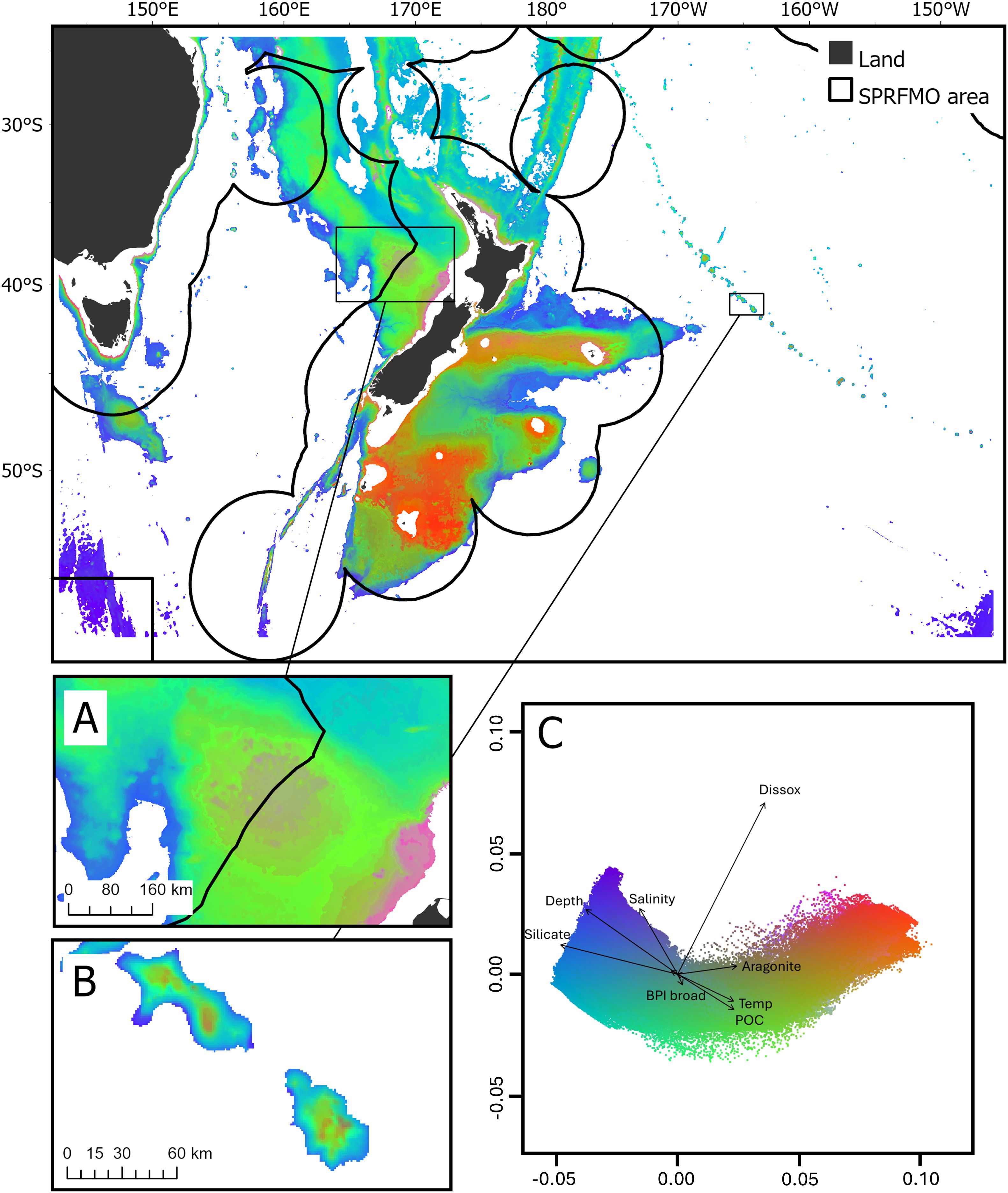
Figure 2. Mean predicted species compositional turnover (over 100 bootstraps) in geographic (top) and Principal Components Analysis (PCA) space (C), derived from Gradient Forest modelling. Colors are based on the first three axes of a PCA analysis so that similarities or differences in color correspond broadly to similarities or differences in mean predicted compositional turnover. (A) Challenger Plateau, (B) Louisville Seamount Chain. Vectors in the PCA space (C) indicate correlations for the environmental predictor variables (Supplementary Table S1) included in the Gradient Forest models. Dissox: dissolved oxygen at depth, Temp: temperature at depth, POC: particulate organic carbon export to the seafloor.
Environmental coverage was high in shallower areas, for example on the Chatham Rise and Campbell Plateau in the New Zealand EEZ and on the Norfolk Ridge, Challenger Plateau (Figure 3A), and on seamounts along the Louisville Seamount Chain (Figure 3B) in the SPRFMO Evaluated Area. In contrast, environmental coverage was lower primarily in deeper areas (deeper than fishable depths, 1,400 m; as per Stephenson et al. (2021); Bennion et al. (2024a), and Bennion et al. (2024c)). For instance, low coverage of the environmental space was estimated in the Bounty Trough (within the New Zealand EEZ) and in the deeper areas across the Louisville Seamount Chain, Challenger Plateau, and South Tasman Rise (within the SPRFMO Evaluated Area) (Figure 3). Unsurprisingly, most training data were in areas with environmental coverage estimates >0.6 (70%). Areas with environmental coverage values <0.2 contained relatively few samples (5% of training data available), model predictions in these spaces should be treated with greater caution and identify spaces which would benefit from sampling effort to reduce uncertainty. Areas of high environmental coverage often overlapped with areas of moderate-high variability in mean compositional turnover (high SD; Stephenson et al., 2022), this reflects the variability in turnover attributable to relative environmental heterogeneity in shallow waters, and in some part, is also likely attributable to comparatively higher sampling effort in areas <2,000 m (Stephenson et al., 2018, 2022).
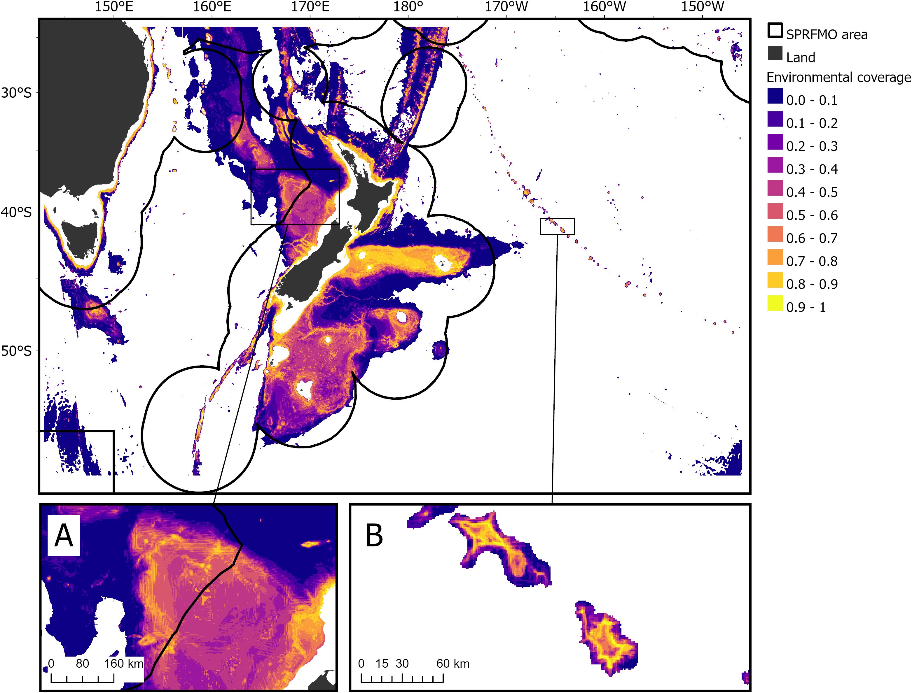
Figure 3. Estimates of environmental coverage between 200 m and 3000 m depth in the study area. Low values of environmental coverage (dark blue approaching 0) indicate parts of the environmental space that contained few samples, meaning greater caution should be placed on the predictions in these areas. Nearly to 70% (>2,300) of model training data was in areas with estimates >0.6, 25% between 0.2-0.6, and 5% in spaces with estimates <0.2. Black lines indicate the boundaries between the SPRFMO Evaluated Area and the multiple Exclusive Economic Zones. The Challenger Plateau (A) and a portion of the Louisville Seamount Chain (B) are shown with insets.
3.2 Describing the VME bioregions
Bioregion 1 was mostly in shallower areas; for example, on the Challenger Plateau and West Norfolk Ridge (Figure 4A); bioregion 2 was also shallow, occurring primarily within New Zealand’s EEZ on the top of plateaus; bioregion 3 followed continental shelf boundaries; bioregions 4 and 5 occurred throughout deeper waters of the study area, while bioregions 6 and 7 were associated with elevated topography, including seamounts (Figure 4B; Supplementary Figures S10-S11). Bioregion 5 was the largest in area, while bioregion 7 was the smallest. While 58% and 67% of the area of bioregions 6 and 7 are contained within the SPRFMO Evaluated Area, <10% of bioregions 1 and 2 were contained within it (Supplementary Table S2). The highest values for POC export to the seafloor, salinity, aragonite saturation, and temperature at depth occurred in bioregion 1 (attributable to its location in relatively shallow areas, Table 2). The highest ruggedness and slope SD was contained within bioregion 6, and the highest values for BPI-broad, and dissolved oxygen were contained within bioregion 7, while the deepest bioregion was bioregion 5 (with the highest silicate concentration also). Text descriptions for the 7-group bioregionalization summarize the environmental characteristics present within each bioregion (Table 3).
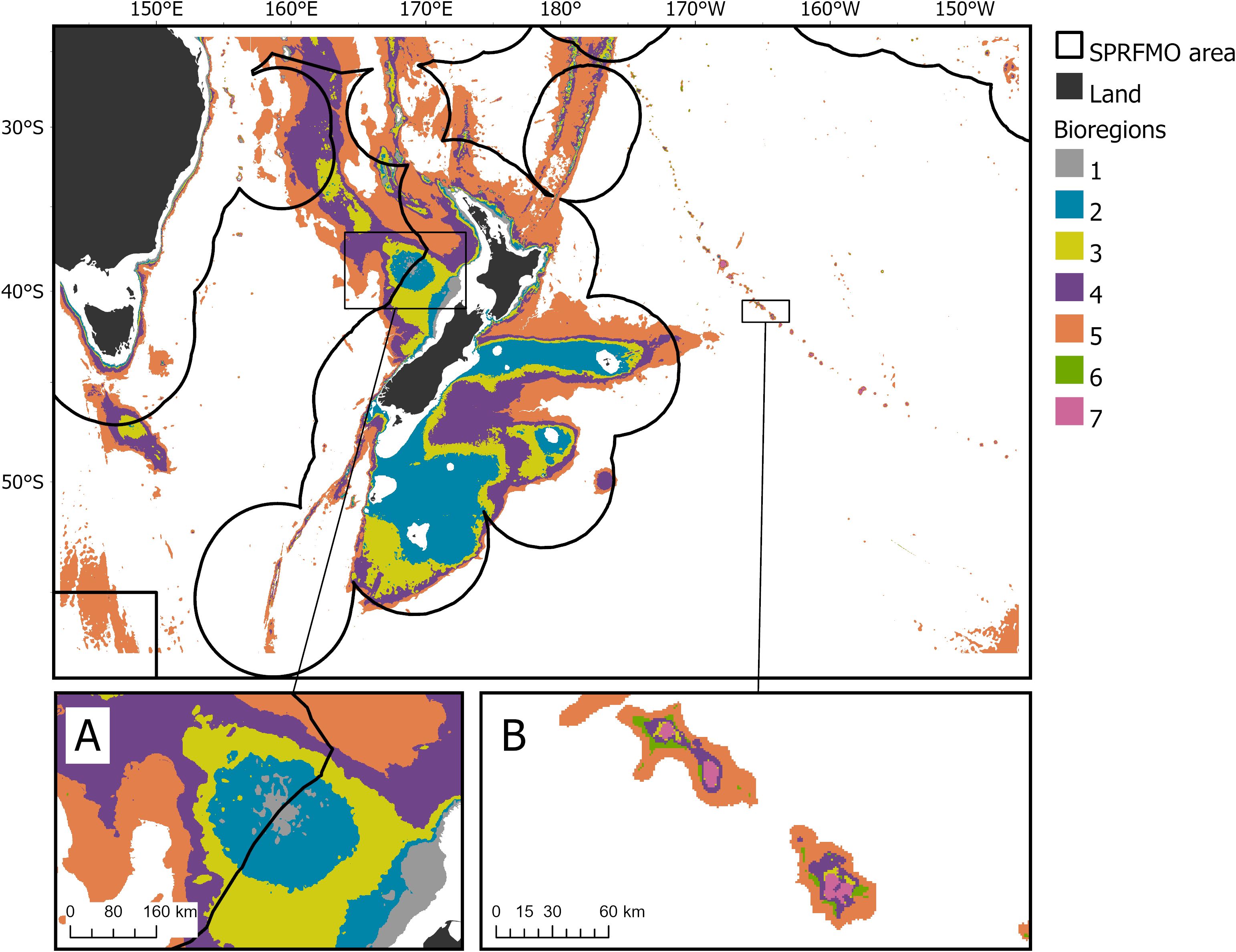
Figure 4. Geographic distribution of the 7-group bioregionalisation derived from the bootstrapped Gradient Forest model fitted with genus-level VME indicator taxa occurrence information. Black lines indicate the boundaries between the SPRFMO Evaluated Area and the multiple Exclusive Economic Zones. The Challenger Plateau (A) and a portion of the Louisville Seamount Chain (B) are shown with insets.
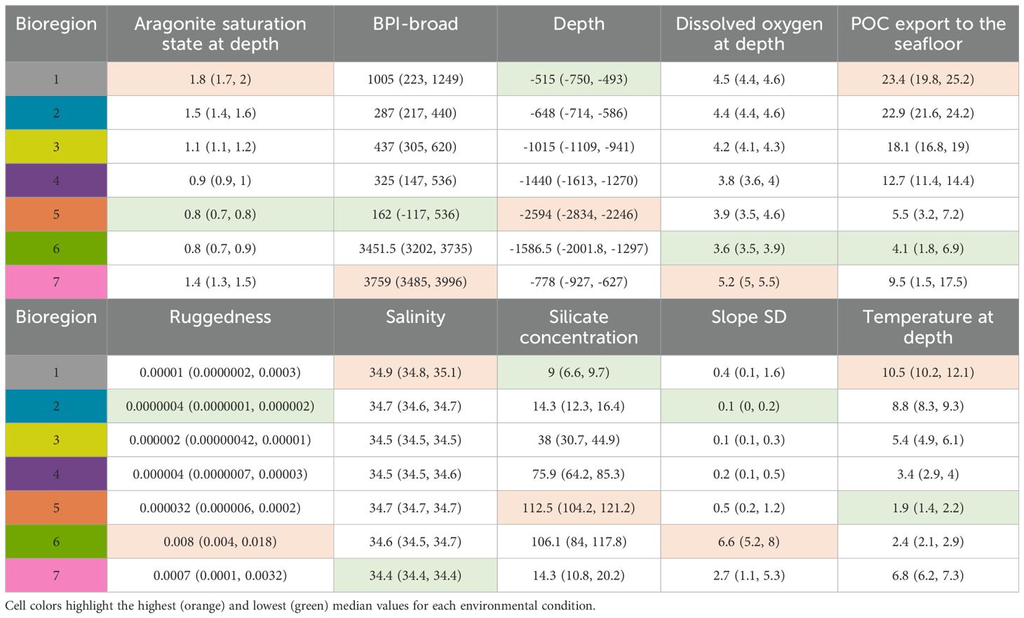
Table 2. Bioregion number (colour matched to Figure 4), descriptions, and median and interquartile range, IQR (25th–75th percentile) of environmental conditions for the 7-group bioregionalisation.
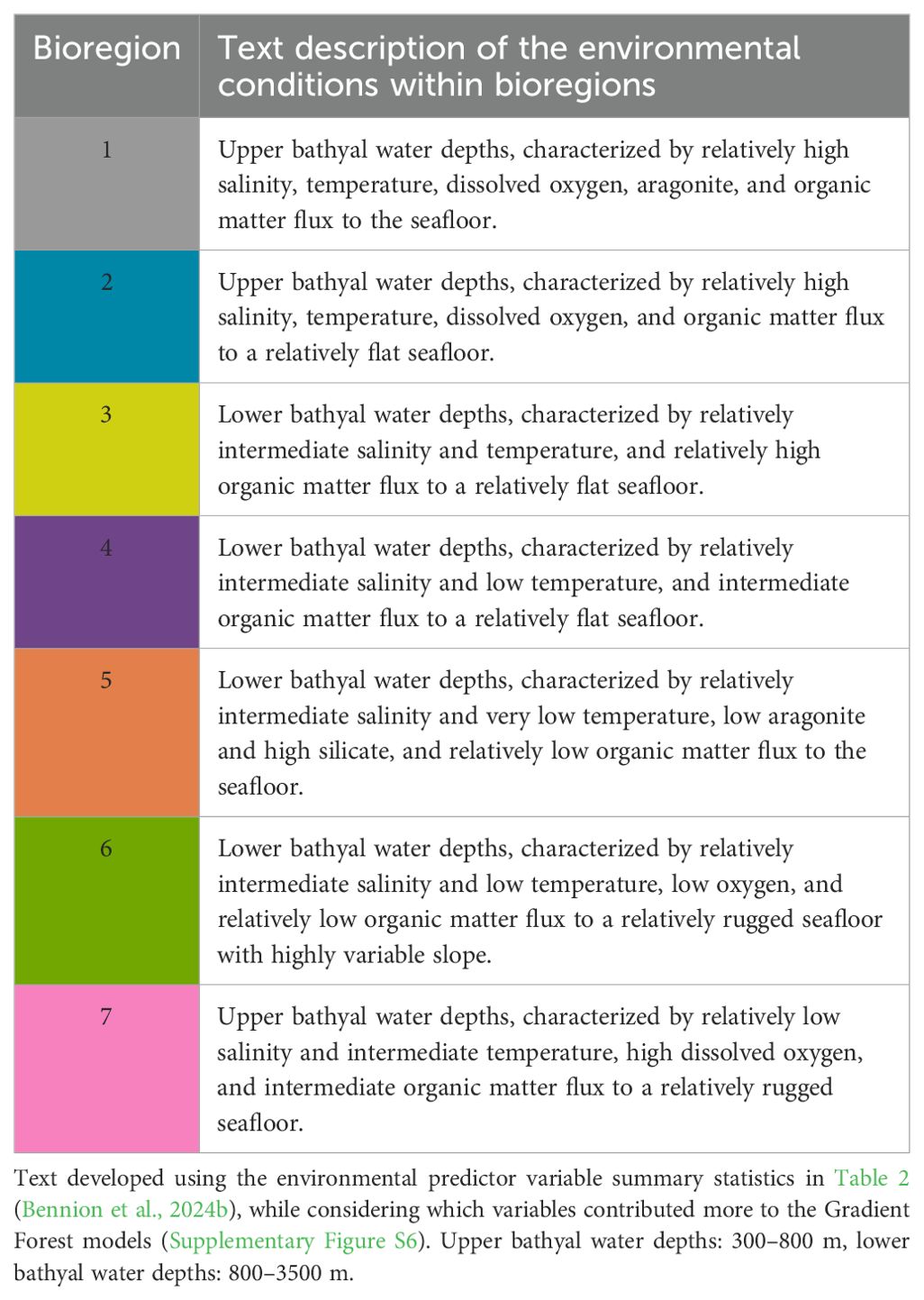
Table 3. Description of bioregions for the 7-group bioregionalisation (bioregion color matched to Figure 4).
For most VME indicator taxa, the majority of ROC-linear transformed suitable habitat was contained within bioregion 5 (the largest bioregion), however, for the stony coral taxa, the proportion of suitable habitat was more variable across other bioregions (Figure 5). For instance, 100% of ROC-linear transformed suitable habitat for Goniocorella dumosa was contained within bioregion 7, almost 50% of ROC-linear transformed suitable habitat for Solenosmilia variabilis was contained within bioregions 6 and 7, while >70% of ROC-linear transformed suitable habitat for Enallopsammia rostrata contained within bioregion 3 (Figure 5A). When ROC-linear transformed suitable habitat for all VME indicator taxa were summed within bioregions, Hydrozoa and Bryozoa contributed ~10% of ROC-linear transformed suitable habitat to most of the bioregions, while other VME indicator taxa, such as Stylasteridae contributed ~10% ROC-linear transformed suitable habitat to the sum value in bioregions 6 and 7 (Figure 5B). Actiniaria contributed little ROC-linear transformed suitable habitat to the sum value of transformed habitat suitability in bioregions (Figure 5B). Following interrogation of the datasets this result was found to be attributed to the ROC-linear transformation of the raw habitat suitability values, where most of the suitable habitat in the SPRFMO Evaluated Area fell below the ROC cut-off and was therefore zero value (i.e., HSI = 0). Note: although these results apply to the SPRFMO Evaluated Area only (Figure 5), the same analyses for the full study area showed similar patterns (Supplementary Figure S12).
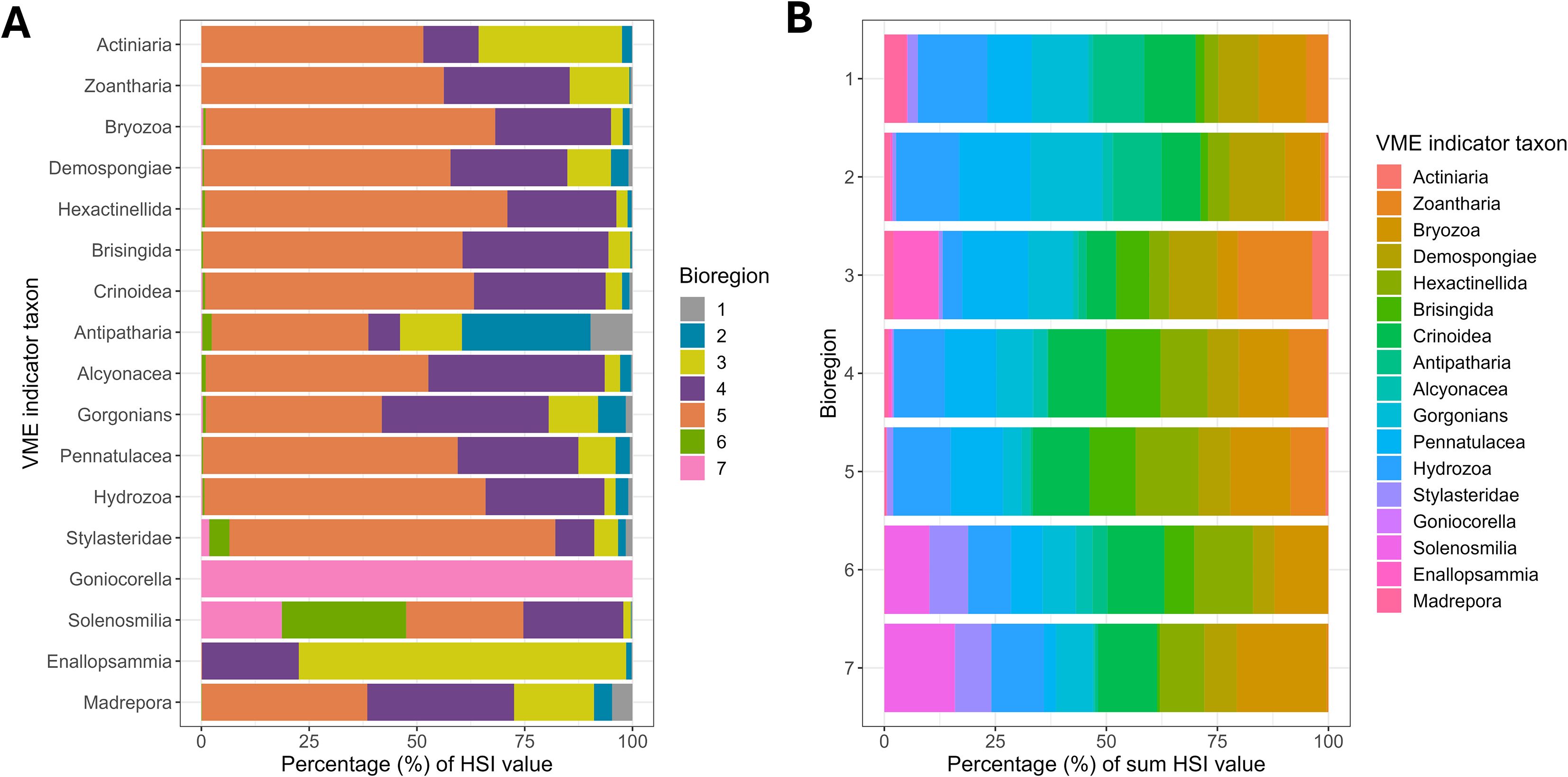
Figure 5. Stacked bar charts show the percentage (%) of ROC-linear transformed suitable habitat (habitat suitability index, HSI) for VME indicator taxa in bioregions for the 7-group bioregionalisation. (A) Shows the percentage of ROC-linear transformed suitable habitat for each VME indicator taxon contained within each bioregion (each bar represents 100% ROC-linear transformed suitable habitat for each VME indicator taxon). Colors are matched to Figure 4. (B) shows the percentage (%) contribution of each VME indicator taxon to the sum of ROC-linear transformed suitable habitat within each bioregion (each bar represents 100% of the summed ROC-linear transformed suitable habitat for all VME indicator taxa). Note: values in these charts were calculated for the SPRFMO Evaluated Area only.
Within bioregion similarity percentages were relatively low (<10%, for all bioregions 1–7) (Supplementary Table S6), which was expected given the high-level of classification (i.e., low level of classification detail). Higher within bioregion similarities (%) would be expected as the classification detail increases, because within group homogeneity would also be expected to increase. For bioregionalizations, which are typically high-level, the SIMPER analysis was therefore more useful for providing an insight into the fauna that contribute to within group similarity. For example, for bioregion 2, Hyalascus (Hexactinellida) contributed 66% to the observed within bioregion similarity, whereas for bioregion 6 Solenosmilia (Scleractinia) contributed 83% to observed within bioregion similarity (Supplementary Table S6). For other bioregions, taxa representing multiple genera contributed to the majority of the within bioregion similarity. Average dissimilarity was highest between bioregions 1 and 6, and lowest between bioregions 4 and 6 (Supplementary Table S7). No single taxon contributed more than 13% to between bioregion dissimilarity. For example, Solenosmilia (Scleractinia) and Conopora (Stylasteridae) contributed the most to the between bioregion dissimilarity for bioregions 1 and 6 (11% and 4% respectively, Supplementary Table S7). While Hyalascus (Hexactinellida) and Goniocorella (Scleractinia) contributed the most to between bioregion dissimilarity for bioregions 1 and 2, at 10% and 6% respectively (Supplementary Table S7).
4 Discussion
A VME-specific bioregionalization with seven environmentally and biologically distinct regions was produced for the western part of the South Pacific Ocean. Bioregionalizations can be useful for identifying biologically relevant geographic boundaries for management units, allowing for targets of representation of different features to be achieved within these units, as well across the full area of interest. For example, representativeness can be evaluated as the percentage of each known habitat type/species’ distribution in each bioregion within an MPA or MPA network. Similarly, consideration of impact, for example from bottom trawling, on species’ distributions can be assessed within bioregional scales since these represent large regions that are biologically and environmentally relatively homogeneous (stable over space and time, Hill et al., 2020) and therefore may also proxy for biological connectivity of species’ populations (Lausche et al., 2021). The decision to use biological data for VME indicator taxa only (as opposed to broader taxonomic groups including other invertebrates and fish, for example) departs from previously produced bioregionalizations for the same area (Dunstan et al., 2018; Stephenson et al., 2023) but is not an entirely novel approach (Ramiro-Sánchez et al., 2023). Individual VME indicator taxon bioregionalizations have been produced in some places; with the concept that they represent distinct VME indicator taxa populations (Summers and Watling, 2021; Watling and Lapointe, 2022). While a seven group bioregionalization for VMEs is described in this study, a 50-class nested community classification has also been produced. Exploration of the ecological relevance of different disaggregation levels could prove useful for informing the use of nested classes for management i.e., within multi-scale approaches (Rowden et al., 2024).
The rationale for producing a combined VME indicator taxa bioregionalization was to generate bioregional boundaries that specifically align to management targets. In SPRFMO, SAIs on VMEs are managed via a series of management areas within which bottom fishing can occur. The bioregions of this “South Pacific VME Bioregionalization” therefore, offer a spatial scale at which future impact assessments can be conducted to determine the effectiveness of the spatial management measures in preventing SAIs. For example, the bioregions can be used to investigate the proportion of suitable habitat or abundance of VME indicator taxa within each bioregion that are afforded protection from bottom fishing (i.e., within areas closed to trawling within management areas). While other bioregionalizations (i.e., Costello et al., 2017) have previously been used for bottom fishing impact assessments in the SPRFMO Evaluated Area (SPRFMO, 2020), the bioregionalization produced here is specific to VME indicator taxa, contains similar, or the same, data to the VME indicator taxa models that were used to design the current trawling closures (i.e., regionally specific), and provides sufficient classification detail within the study area. In addition to any future impact assessments, the South Pacific VME Bioregionalization could potentially be used to inform the refinement of the boundaries of the current bottom trawling management areas to achieve protection targets (e.g., SPRFMO CMM03–2024 mandates a minimum of 70% protection of suitable habitat for each modelled VME indicator taxa), and the boundaries of fisheries management areas in which they sit (e.g., to better align the current fishery management areas with ecological spatial scales, in addition to those that relate to the target fish species). Furthermore, for impact assessments that directly assess SAIs, such as the measure of relative benthic status that is used by SPRFMO (Pitcher et al., 2017; SPRFMO, 2020), these assessments could now be made at the bioregion scale as well as the smaller spatial scales that are currently used, as part of a multi-spatial scale assessment.
While bioregions have practical applications, bioregional boundaries can also be useful for exploring biodiversity patterns and ecological theory e.g., biodiversity organization within bioregions (Bernardo-Madrid et al., 2025). For example, bioregions can be used to test connectivity hypotheses, and turnover functions can be used to explore how turnover is modulated by certain environmental conditions. In this way, steep slopes in turnover functions can be used to infer compositional tipping points along environmental gradients where species turnover is rapid in response to a certain environmental condition (Ellis et al., 2012; Stephenson et al., 2022).
The selection of seven bioregions for the South Pacific Ocean that characterize distinct VME assemblages, and the environmental conditions that support them, was supported by a variety of statistical and descriptive analyses. Ultimately, the selection of the ‘appropriate’ number of bioregions is somewhat subjective and does not necessarily have to be supported statistically; appropriateness for spatial planning should be used to guide the choice also (Beger et al., 2020). This choice does not influence the ecological relevance of the bioregional boundaries given the data and underlying model used to create them, instead the resolution (i.e., number of groups or classes) denotes ecological relevance at different scales (Spalding et al., 2007). For example, a fine classification (higher number of classes or groups) corresponds to the community level (Stephenson et al., 2022), while an even finer classification may represent populations/precise habitats (Koen-Alonso et al., 2019). In the North Atlantic Ocean (including the Northwest Atlantic Fisheries Organization (NAFO) RFMO area), work on VME-specific bioregionalizations produced three separate scales: 1) bioregions, 2) ecosystem production units (EPUs), and 3) ecoregions (Koen-Alonso et al., 2019). Bioregions are considered to represent “major marine communities/food web systems”, while EPUs are subunits distinguished by distinct productivity, and an ecoregion is finer still, corresponding to a “broadly defined seascape and/or major habitat type” (Koen-Alonso et al., 2019). In this way, applying separate scales depending on the management objective is possible. For instance, it may be more appropriate to consider productivity at a local level to manage certain activities/impacts, while the bioregional scale may be applicable for multiple impacts that accumulate over large spatial scales (Whitehead et al., 2017). Nevertheless, the FAO (2009) guidelines on the management of deep-sea fisheries in the high seas provides various criteria to identify VMEs, including ‘functional significance of the habitat’. Productivity and functionality go hand in hand, therefore scales that correspond directly to productivity may be informative for some assessments. Effective marine spatial planning can be flexible, and the use of decision-support tools to conduct impact assessments and inform management measures provides one avenue to consider multiple spatial scales with ease (Lagabrielle et al., 2018; Stephenson et al., 2024b). The seven group bioregionalization was deemed appropriate for the study area, based on the data used to train the models, yet the hierarchical approach used means that nested classes are available (up to 50 classes) to support multi-scale assessments. This classification could allow for the production of additional spatial scales that correspond to the bioregions e.g., ecological production units and ecoregions (Koen-Alonso et al., 2019). Moreover, the methods used are reproducible and should further data become available, the classification and subsequent bioregionalization could be validated (Stephenson et al., 2024c) and updated (Stephenson, 2023).
Spatial predictive models are subject to the limitations and biases of the data used to train them (Robinson et al., 2011). While some of these issues can be managed, some cannot, and all should be carefully considered when using the outputs to inform spatial management e.g., assessing the areas within and outside the environmental ranges of observed data (Stephenson et al., 2021; Vinha et al., 2024); referred to herein as ‘environmental coverage’. The GF model used here was trained with presence-only information. Ideally, the model would be trained with information of true presence-absence or abundance-absence data (Vinha et al., 2024), but these data are rarely available for deep-sea ecosystems at the scale required to generate robust models (Bridges et al., 2023). The presence-only information used here comes with limitations (e.g., catchability and biases towards fished areas) and while high-quality seafloor imagery data does exist for the study area, and has been used to generate abundance models for VME indicator taxa (Bennion et al., 2024c), the presence-only information provides a more extensive number of records for VME indicators than imagery data alone (>3,000 unique locations compared to <900). Furthermore, the taxonomic resolution of the imagery data (typically at levels coarser than genera) potentially limits their usefulness to produce a more robust bioregionalization than the one produced here, given that bioregionalizations should ideally be based on data at the species or genera level. Nonetheless, despite the coarser taxonomic resolution of imagery data, it would be useful in the first instance to explore an independent validation of the South Pacific VME Bioregionalization in a manner like that described by Stephenson et al. (2024c); analogous to the evaluations carried out on habitat suitability models for VME indicator taxa in the same region (Bennion et al., 2024a; Bowden et al., 2021).
Environmental characteristics are the foundation of bioregionalizations, including the one presented here. While the environmental variable datasets used here represent best available data at the scale of the study area, several important variables are missing (Bennion et al., 2024c). Substrate type is the determinant variable for many benthic habitat-forming species, a trait shared by many VME indicator taxa; an absence of high-quality substrate type data for the deep sea (beyond highly local scales i.e., individual seamounts) increases uncertainty in predictive model outputs (Bowden et al., 2021). Several variables included in the model, however, are provided as substrate type proxies (slope SD, ruggedness, and BPI-broad) but it is likely that fine-resolution substrate type information would have a considerable impact on the model’s predictive power. The availability and use of other environmental datasets (e.g., variation in sea surface temperature as a proxy for the location of oceanic fronts) would also likely improve the model. Updating the South Pacific VME Bioregionalization should therefore be considered if: 1) improved environmental datasets become available; and 2) substantially more (or higher taxonomic resolution) biological data become available (especially within the SPRFMO Evaluated Area).
Despite the exclusion of information for non-VME indicator taxa, the bioregionalization generated here is broadly similar to the Seafloor Bioregionalization for New Zealand (Stephenson et al., 2023), which includes many of the same areas in the New Zealand EEZ. This visual assessment provides some confidence in the bioregions produced here because despite differences in the biological and environmental datasets used, we would expect the bioregionalizations to share similarities. That is, the environmental conditions that disaggregate seafloor communities (seafloor topography, water masses) will be broadly similar, whether taxa constitute VME indicators or not. Therefore, we believe that until a validation and/or an update is possible, the South Pacific VME Bioregionalization could be used cautiously (supported by spatial estimates of confidence to account for model uncertainty (standard deviation of compositional turnover) and data gaps (environmental coverage)) as an alternative spatial scale at which to evaluate the effectiveness of SPRFMO’s spatial management measures.
It is has recently been noted that there is poor coordination across RFMOs with respect to their efforts to align approaches for assessing SAIs on VMEs (Kaikkonen et al., 2024). The VME bioregionalization approach presented here could be replicated in other parts of the globe, enabling a form of alignment across RFMOs, while allowing impact assessments to better consider representativeness of groups of VME species and communities, and thereby facilitate better management outcomes.
Data availability statement
The original contributions presented in the study are publicly available. The NIWA open data portal (https://data-niwa.opendata.arcgis.com/datasets) provides access to the species occurrence data used in this study. Environmental datasets can be sourced from various locations detailed in Table S1 in the Supplementary Material and are openly available (reduced extent) from https://datadryad.org/dataset/doi:10.5061/dryad.41ns1rnht (Anderson et al., 2022). Much of the R code used to develop this work can be found in an online tutorial produced by developers of the gradientForest package (https://gradientforest.r-forge.r-project.org/biodiversity-survey.pdf). Additional R code used in this study is available in the GitHub open repository: https://github.com/Fabrice-Stephenson/VME_Bioregionalisation.
Author contributions
MB: Conceptualization, Formal Analysis, Investigation, Methodology, Writing – original draft, Writing – review & editing. AR: Conceptualization, Funding acquisition, Investigation, Writing – original draft, Writing – review & editing, Methodology. BM: Funding acquisition, Methodology, Project administration, Writing – review & editing. OA: Data curation, Funding acquisition, Writing – review & editing. JT: Methodology, Writing – review & editing. SG: Data curation, Methodology, Writing – review & editing. FS: Conceptualization, Data curation, Methodology, Writing – review & editing.
Funding
The author(s) declared that financial support was received for this work and/or its publication. Funding for this study was provided by Fisheries New Zealand (Ministry for Primary Industries) to the National Institute of Water and Atmospheric Research Ltd. (NIWA) under contract SPR2023-01. Funding for the writing of this study was provided by NIWA Fisheries Centre under the Strategic Science Investment Fund project FINC2501.
Acknowledgments
Foremost, we want to thank all those who have contributed to the collection and maintenance of datasets that were used in this work. We also thank Alexander Arkhipkin (Fisheries New Zealand) and the members of the South Pacific Working Group for discussions that improved this work. This manuscript builds on a report available online from https://sprfmo.int/ (SC 12 – DW 11_rev1; Bennion et al., 2024b).
Conflict of interest
The author(s) declared that this work was conducted in the absence of any commercial or financial relationships that could be construed as a potential conflict of interest.
The reviewer GG-M declared a past co-authorship with the author AR to the handling editor.
The authors declare that this study received funding from Fisheries New Zealand. The funder was not involved in the study design, collection, analysis, interpretation of data, the writing of this article or decision to submit the article for publication. The funder was involved in the South Pacific Working Group process and discussions therein. The funder was responsible for the formal recommendations that resulted from this work, but which are not included in this article, that were made to the Scientific Committee of SPRFMO to consider.
Generative AI statement
The author(s) declare that no Generative AI was used in the creation of this manuscript.
Any alternative text (alt text) provided alongside figures in this article has been generated by Frontiers with the support of artificial intelligence and reasonable efforts have been made to ensure accuracy, including review by the authors wherever possible. If you identify any issues, please contact us.
Publisher’s note
All claims expressed in this article are solely those of the authors and do not necessarily represent those of their affiliated organizations, or those of the publisher, the editors and the reviewers. Any product that may be evaluated in this article, or claim that may be made by its manufacturer, is not guaranteed or endorsed by the publisher.
Supplementary material
The Supplementary Material for this article can be found online at: https://www.frontiersin.org/articles/10.3389/fevo.2025.1670027/full#supplementary-material
References
Anderson O. F., Stephenson F., Behrens E., and Rowden A. A. (2022). Predicting the effects of climate change on deep-water coral distribution around New Zealand—Will there be suitable refuges for protection at the end of the 21st century? Global Change Biol. 28, 6556–6576. doi: 10.1111/gcb.16389
Beger M., Wendt H., Sullivan J., Mason C., Legrand J., Davey K., et al. (2020). National-scale marine bioregions for the Southwest Pacific. Mar. pollut. Bull. 150, 110710. doi: 10.1016/j.marpolbul.2019.110710
Bennion M., Anderson O. F., Rowden A. A., Bowden D. A., Geange S. W., and Stephenson F. (2024a). Evaluation of the full set of habitat suitability models for vulnerable marine ecosystem indicator taxa in the South Pacific high seas. Fish. Manage. Ecol., e12700. doi: 10.1111/fme.12700
Bennion M., Rowden A. A., Anderson O., Bowden D. A., Clark M. R., Althaus F., et al. (2024c). The use of image-based data and abundance modelling approaches for predicting the location of vulnerable marine ecosystems in the South Pacific Ocean. Fish. Manage. Ecol., e12751. doi: 10.1111/fme.12751
Bennion M., Rowden A., Anderson O., Moore B., Stephenson F., Tablada J., et al. (2024b). “Development of a bioregionalisation for VME indicator taxa. SC12–DW11_rev1,” in 12th Meeting of the Scientific Committee (South Pacific Regional Fisheries Management Organisation (SPRFMO).
Bernardo-Madrid R., González-Suárez M., Rosvall M., Rueda M., Revilla E., Carrete M., et al. (2025). A general rule on the organization of biodiversity in Earth’s biogeographical regions. Nat. Ecol. Evol. 9, 1193–1204. doi: 10.1038/s41559-025-02724-5
Bowden D. A., Anderson O. F., Rowden A. A., Stephenson F., and Clark M. R. (2021). Assessing habitat suitability models for the deep sea: is our ability to predict the distributions of seafloor fauna improving? Front. Mar. Sci. 8. doi: 10.3389/fmars.2021.632389
Bridges A. E. H., Barnes D. K. A., Bell J. B., Ross R. E., Voges L., and Howell K. L. (2023). Filling the data gaps: Transferring models from data-rich to data-poor deep-sea areas to support spatial management. J. Environ. Manage. 345, 118325. doi: 10.1016/j.jenvman.2023.118325
Brito-Morales I., Schoeman D. S., Everett J. D., Klein C. J., Dunn D. C., García Molinos J., et al. (2022). Towards climate-smart, three-dimensional protected areas for biodiversity conservation in the high seas. Nat. Climate Change 12, 402–407. doi: 10.1038/s41558-022-01323-7
Chamberlain S. and Vanhoorne B. (2023). worrms: World Register of Marine Species (WoRMS) Client. 0.4.3 ed (R cran).
Clark M. R., Althaus F., Schlacher T. A., Williams A., Bowden D. A., and Rowden A. A. (2016). The impacts of deep-sea fisheries on benthic communities: a review. ICES. J. Mar. Sci. 73, i51–i69. doi: 10.1093/icesjms/fsv123
Costello M. J., Tsai P., Wong P. S., Cheung A. K. L., Basher Z., and Chaudhary C. (2017). Marine biogeographic realms and species endemicity. Nat. Commun. 8, 1057. doi: 10.1038/s41467-017-01121-2
Day J., Dudley N., Hockings M., Holmes G., Laffoley D. D. A., Stolton S., et al. (2012). Guidelines for applying the IUCN protected area management categories to marine protected areas (IUCN).
Dunstan P. K., Hayes D., Woolley S., Allain V., Leduc D., Rowden A. A., et al. (2018). Bioregions of the South West Pacific Ocean (Australia: CSIRO).
Elith J. and Leathwick J. R. (2009). Species distribution models: ecological explanation and prediction across space and time. Annu. Rev. Ecol. Evol. Syst. 40, 677–697. doi: 10.1146/annurev.ecolsys.110308.120159
Ellis N., Smith S. J., and Pitcher C. R. (2012). Gradient forests: calculating importance gradients on physical predictors. Ecology 93, 156–168. doi: 10.1890/11-0252.1
Falco F. L., Preiss-Bloom S., and Dayan T. (2022). Recent evidence of scale matches and mismatches between ecological systems and management actions. Curr. Landscape Ecol. Rep. 7, 104–115. doi: 10.1007/s40823-022-00076-5
FAO (2009). International Guidelines for the Management of Deep-sea Fisheries in the High Seas (Rome, Italy).
Ferrier S. and Guisan A. (2006). Spatial modelling of biodiversity at the community level. J. Appl. Ecol. 43, 393–404. doi: 10.1111/j.1365-2664.2006.01149.x
Foster N. L., Rees S., Langmead O., Griffiths C., Oates J., and Attrill M. J. (2017). Assessing the ecological coherence of a marine protected area network in the Celtic Seas. Ecosphere 8, e01688. doi: 10.1002/ecs2.1688
Geange S. W., Rowden A. A., Cryer M., and Bock T. D. (2020). “Developing a multi-taxonomic level list of VME indicator taxa for the SPRFMO Convention Area. SC8-DW11,” in 8th Meeting of the Scientific Committee (South Pacific Regional Fisheries Management Organisation (SPRFMO).
Georgian S. E., Anderson O. F., and Rowden A. A. (2019). Ensemble habitat suitability modeling of vulnerable marine ecosystem indicator taxa to inform deep-sea fisheries management in the South Pacific Ocean. Fish. Res. 211, 256–274. doi: 10.1016/j.fishres.2018.11.020
Grorud-Colvert K., Sullivan-Stack J., Roberts C., Constant V., Horta E Costa B., Pike E. P., et al. (2021). The MPA Guide: A framework to achieve global goals for the ocean. Science 373, eabf0861. doi: 10.1126/science.abf0861
Gros C., Jansen J., Dunstan P. K., Welsford D. C., and Hill N. A. (2022). Vulnerable, but still poorly known, marine ecosystems: how to make distribution models more relevant and impactful for conservation and management of VMEs? Front. Mar. Sci. 9. doi: 10.3389/fmars.2022.870145
Guarinello M. L., Shumchenia E. J., and King J. W. (2010). Marine habitat classification for ecosystem-based management: A proposed hierarchical framework. Environ. Manage. 45, 793–806. doi: 10.1007/s00267-010-9430-5
Hennig C. (2019). fpc R package. v.2.2-13. Available online at: https://rdocumentation.org/packages/fpc/versions/2.2-13.
Hesselbarth M. H. K., Sciaini M., With K. A., Wiegand K., and Nowosad J. (2019). landscapemetrics: an open-source R tool to calculate landscape metrics. Ecography 42, 1648–1657. doi: 10.1111/ecog.04617
Hewitt J., Stephenson F., Thrush S., Low J., Pilditch C., Gladstone-Gallagher R., et al. (2024). How the Scale of Spatial Management Can Reduce Risks of Mis-Management in the Marine Environment, SSRN 4888714.
Hijmans R. J., Van Etten J., Cheng J., Mattiuzzi M., Sumner M., Greenberg J. A., et al. (2015). Package ‘raster’ Vol. 734 (R package), 473.
Hill N. A., Foster S. D., Duhamel G., Welsford D., Koubbi P., and Johnson C. R. (2017). Model-based mapping of assemblages for ecology and conservation management: A case study of demersal fish on the Kerguelen Plateau. Diversity Distrib. 23, 1216–1230. doi: 10.1111/ddi.12613
Hill N., Woolley S. N. C., Foster S., Dunstan P. K., Mckinlay J., Ovaskainen O., et al. (2020). Determining marine bioregions: A comparison of quantitative approaches. Methods Ecol. Evol. 11, 1258–1272. doi: 10.1111/2041-210X.13447
Kaikkonen L., Amaro T., Auster P. J., Bailey D. M., Bell J. B., Brandt A., et al. (2024). Improving impact assessments to reduce impacts of deep-sea fisheries on vulnerable marine ecosystems. Mar. Policy 167, 106281. doi: 10.1016/j.marpol.2024.106281
Klanten O. S., Gall M., Barbosa S. S., Hart M. W., Keever C. C., Puritz J. B., et al. (2023). Population connectivity across east Australia's bioregions and larval duration of the range-extending sea star. Aquat. Conserv.: Mar. Freshw. Ecosyst. 33, 1061–1078. doi: 10.1002/aqc.3973
Koen-Alonso M., Pepin P., Fogarty M. J., Kenny A., and Kenchington E. (2019). The Northwest Atlantic Fisheries Organization Roadmap for the development and implementation of an Ecosystem Approach to Fisheries: structure, state of development, and challenges. Mar. Policy 100, 342–352. doi: 10.1016/j.marpol.2018.11.025
Lagabrielle E., Lombard A. T., Harris J. M., and Livingstone T.-C. (2018). Multi-scale multi-level marine spatial planning: A novel methodological approach applied in South Africa. PloS One 13, e0192582. doi: 10.1371/journal.pone.0192582
Lausche B., Laur A., and Collins M. (2021). Marine Connectivity Conservation “Rules of Thumb” For MPA and MPA Network Design (IUCN WCPA Connectivity Conservation Specialist Group's Marine Connectivity Working Group).
Leathwick J., Snelder T., Chadderton W., Elith J., Julian K., and Ferrier S. (2011). Use of generalised dissimilarity modelling to improve the biological discrimination of river and stream classifications. Freshw. Biol. 56, 21–38. doi: 10.1111/j.1365-2427.2010.02414.x
Mackay K., Mitchell J., Neil H., and Mackay E. (2015). New Zealand's marine realm. NIWA chart, Miscellaneous Series.
Maechler M. (2019). Finding groups in data: Cluster analysis extended Rousseeuw et al. R package version, 2. 242–248.
Moilanen A., Runge M. C., Elith J., Tyre A., Carmel Y., Fegraus E., et al. (2006). Planning for robust reserve networks using uncertainty analysis. Ecol. Model. 199, 115–124. doi: 10.1016/j.ecolmodel.2006.07.004
Oksanen J., Blanchet F. G., Kindt R., Legendre P., Minchin P. R., O’Hara R., et al. (2013). Package ‘vegan’ (Community ecology package), 1–295.
Parker S. J. and Bowden D. A. (2010). Identifying taxonomic groups vulnerable to bottom longline fishing gear in the Ross Sea region. CCAMLR. Sci. 17, 105–127.
Parker S. J., Penney A. J., and Clark M. R. (2009). Detection criteria for managing trawl impacts on vulnerable marine ecosystems in high seas fisheries of the South Pacific Ocean. Mar. Ecol. Prog. Ser. 397, 309–317. doi: 10.3354/meps08115
Phillips S. J., Dudík M., Elith J., Graham C. H., Lehmann A., Leathwick J., et al. (2009). Sample selection bias and presence-only distribution models: implications for background and pseudo-absence data. Ecol. Appl. 19, 181–197. doi: 10.1890/07-2153.1
Pinkerton M. H., Smith A. N. H., Raymond B., Hosie G. W., Sharp B., Leathwick J. R., et al. (2010). Spatial and seasonal distribution of adult Oithona similis in the Southern Ocean: Predictions using boosted regression trees. Deep. Sea. Res. Part I.: Oceanogr. Res. Papers. 57, 469–485. doi: 10.1016/j.dsr.2009.12.010
Pitcher C. R., Ellis N., Jennings S., Hiddink J. G., Mazor T., Kaiser M. J., et al. (2017). Estimating the sustainability of towed fishing-gear impacts on seabed habitats: a simple quantitative risk assessment method applicable to data-limited fisheries. Methods Ecol. Evol. 8, 472–480. doi: 10.1111/2041-210X.12705
Pitcher R. C., Ellis N., and Smith S. J. (2011). Example analysis of biodiversity survey data with R package gradientForest.
Positteam (2023). RStudio: Integrated Development Environment for R (Boston, MA: Posit Software, PBC). Available online at: http://www.posit.co/.
Ramiro-Sánchez B., Woolley S., and Leroy B. (2023). Bioregionalization of the SIOFA area based on vulnerable marine ecosystem indicator taxa (Project PAE2021-01) (France: Muséum d’Histoire Naturelle).
Roberts K. E., Valkan R. S., and Cook C. N. (2018). Measuring progress in marine protection: A new set of metrics to evaluate the strength of marine protected area networks. Biol. Conserv. 219, 20–27. doi: 10.1016/j.biocon.2018.01.004
Robinson L. M., Elith J., Hobday A. J., Pearson R. G., Kendall B. E., Possingham H. P., et al. (2011). Pushing the limits in marine species distribution modelling: lessons from the land present challenges and opportunities. Global Ecol. Biogeogr. 20, 789–802. doi: 10.1111/j.1466-8238.2010.00636.x
Robinson N. M., Nelson W. A., Costello M. J., Sutherland J. E., and Lundquist C. J. (2017). A Systematic review of marine-based species distribution models (SDMs) with recommendations for best practice. Front. Mar. Sci. 4. doi: 10.3389/fmars.2017.00421
Rowden A., Tablada J., and Arkhipkin A. (2024). “A review of information to assist in defining thresholds for significant adverse impact on vulnerable marine ecosystems,” in 12th Meeting of the Scientific Committee of the South Pacific Regional Fisheries Management Organisation, Lima, Peru.
Smith A. N., Duffy C., Anthony J., and Leathwick J. R. (2013). Predicting the distribution and relative abundance of fishes on shallow subtidal reefs around New Zealand (Wellington, NZ: Department of Conservation).
Snelder T. H., Leathwick J. R., Dey K. L., Rowden A. A., Weatherhead M. A., Fenwick G. D., et al. (2007). Development of an ecologic marine classification in the New Zealand region. Environ. Manage. 39, 12–29. doi: 10.1007/s00267-005-0206-2
Spalding M. D., Fox H. E., Allen G. R., Davidson N., Ferdaña Z. A., Finlayson M., et al. (2007). Marine ecoregions of the world: A bioregionalization of coastal and shelf areas. BioScience 57, 573–583. doi: 10.1641/b570707
SPRFMO (2020). “Cumulative Bottom Fishery Impact Assessment for Australian and New Zealand bottom fisheries in the SPRFMO Convention Area 2020. SC8-DW07 rev 1,” in 8th Meeting of the Scientific Committee, Wellington, NZ (South Pacific Regional Fisheries Management Organisation (SPRFMO).
SPRFMO (2023). Conservation and Management Measure for the Management of Bottom Fishing in the SPRFMO Convention Area. CMM 03-2023 (Wellington, NZ: South Pacific Regional Fisheries Management Organisation (SPRFMO).
Stephenson F. (2023). Developing a maintenance framework for the NZSCC (Wellington, NZ: Ocean Analytics report prepared for the Department of Conservation).
Stephenson F., Bowden D. A., Rowden A. A., Anderson O. F., Clark M. R., Bennion M., et al. (2024a). Using joint species distribution modelling to predict distributions of seafloor taxa and identify vulnerable marine ecosystems in New Zealand waters. Biodivers. Conserv. 33, 3103–3127. doi: 10.1007/s10531-024-02904-y
Stephenson F., Goetz K., Sharp B. R., Mouton T. L., Beets F. L., Roberts J., et al. (2020a). Modelling the spatial distribution of cetaceans in New Zealand waters. Diversity Distrib. 26, 495–516. doi: 10.1111/ddi.13035
Stephenson F., Leathwick J. R., Francis M. P., and Lundquist C. J. (2020b). A New Zealand demersal fish classification using Gradient Forest models. New Z. J. Mar. Freshw. Res. 54, 60–85. doi: 10.1080/00288330.2019.1660384
Stephenson F., Leathwick J. R., Geange S. W., Bulmer R. H., Hewitt J. E., Anderson O. F., et al. (2018). Using Gradient Forests to summarize patterns in species turnover across large spatial scales and inform conservation planning. Diversity Distrib. 24, 1641–1656. doi: 10.1111/ddi.12787
Stephenson F., Leathwick J. R., Geange S., Moilanen A., and Lundquist C. J. (2024b). Contrasting performance of marine spatial planning for achieving multiple objectives at national and regional scales. Ocean. Coast. Manage. 248, 106978. doi: 10.1016/j.ocecoaman.2023.106978
Stephenson F., Rowden A. A., Anderson O. F., Pitcher C. R., Pinkerton M. H., Petersen G., et al. (2021). Presence-only habitat suitability models for vulnerable marine ecosystem indicator taxa in the South Pacific have reached their predictive limit. ICES. J. Mar. Sci. 78, 2830–2843. doi: 10.1093/icesjms/fsab162
Stephenson F., Rowden A. A., Brough T., Petersen G., Bulmer R. H., Leathwick J. R., et al. (2022). Development of a seafloor community classification for the New Zealand region using a gradient forest approach. Front. Mar. Sci. 8. doi: 10.3389/fmars.2021.792712
Stephenson F., Rowden A. A., Tablada J., Tunley K., Brough T., Lundquist C. J., et al. (2023). A seafloor bioregionalisation for New Zealand. Ocean. Coast. Manage. 242, 106688. doi: 10.1016/j.ocecoaman.2023.106688
Stephenson F., Tablada J., Rowden A. A., Bulmer R., Bowden D. A., and Geange S. W. (2024c). Independent statistical validation of the New Zealand Seafloor Community Classification. Aquat. Conserv.: Mar. Freshw. Ecosyst. 34, e4114. doi: 10.1002/aqc.4114
Summers N. and Watling L. (2021). Upper Bathyal Pacific Ocean biogeographic provinces from octocoral distributions. Prog. Oceanogr. 191, 102509. doi: 10.1016/j.pocean.2020.102509
UNESCO (2009). Global Open Oceans and Deep Seabed (GOODS) – Biogeo-graphic Classification. IOC Technical Series (Paris: UNESCO-IOC).
UNGA (2006). “Sustainable fisheries, including through the 1995 Agreement for the Implementation of the Provisions of the United Nations Convention on the Law of the Sea of 10 December 1982 relating to the Conservation and Management of Straddling Fish Stocks and Highly Migratory Fish Stocks, and related instruments,” in UNGA 61st Session (New York, United States of America: United Nations General Assembly).
UNGA (2009). “Sustainable fisheries, including through the 1995 Agreement for the Implementation of the Provisions of the United Nations Convention on the Law of the Sea of 10 December 1982 relating to the Conservation and Management of Straddling Fish Stocks and Highly Migratory Fish Stocks, and related instruments,” in UNGA 64th Session (New York, United States of America: United Nations General Assembly).
UNGA (2011). “Sustainable fisheries, including through the 1995 Agreement for the Implementation of the Provisions of the United Nations Convention on the Law of the Sea of 10 December 1982 relating to the Conservation and Management of Straddling Fish Stocks and Highly Migratory Fish Stocks, and related instruments,” in UNGA 66th Session (New York, United States of America: United Nations General Assembly).
Vinha B., Murillo F. J., Schumacher M., Hansteen T. H., Schwarzkopf F. U., Biastoch A., et al. (2024). Ensemble modelling to predict the distribution of vulnerable marine ecosystems indicator taxa on data-limited seamounts of Cabo Verde (NW Africa). Diversity Distrib. 30, e13896. doi: 10.1111/ddi.13896
Watling L. and Lapointe A. (2022). Global biogeography of the lower bathyal (700–3000 m) as determined from the distributions of cnidarian anthozoans. Deep. Sea. Res. Part I.: Oceanogr. Res. Papers. 181, 103703. doi: 10.1016/j.dsr.2022.103703
Whitehead A. L., Kujala H., and Wintle B. A. (2017). Dealing with cumulative biodiversity impacts in strategic environmental assessment: A new frontier for conservation planning. Conserv. Lett. 10, 195–204. doi: 10.1111/conl.12260
Wickham H., Averick M., Bryan J., Chang W., Mcgowan L. D. A., François R., et al. (2019). Welcome to the tidyverse. J. Open Source Softw. 4, 1686. doi: 10.21105/joss.01686
Keywords: marine spatial planning, fisheries management, high seas and deep sea ecosystems, Vulnerable Marine Ecosystem (VME), bioregion
Citation: Bennion M, Rowden AA, Moore BR, Anderson OF, Tablada J, Geange SW and Stephenson F (2025) Development of the South Pacific Vulnerable Marine Ecosystem bioregionalisation. Front. Ecol. Evol. 13:1670027. doi: 10.3389/fevo.2025.1670027
Received: 21 July 2025; Accepted: 11 November 2025; Revised: 06 November 2025;
Published: 08 December 2025.
Edited by:
Marco C. Brustolin, Norwegian Institute of Marine Research (IMR), NorwayReviewed by:
Genoveva Gonzalez-Mirelis, Norwegian Institute of Marine Research (IMR), NorwayDanilo Candido Vieira, University of São Paulo, Brazil
Copyright © 2025 Bennion, Rowden, Moore, Anderson, Tablada, Geange and Stephenson. This is an open-access article distributed under the terms of the Creative Commons Attribution License (CC BY). The use, distribution or reproduction in other forums is permitted, provided the original author(s) and the copyright owner(s) are credited and that the original publication in this journal is cited, in accordance with accepted academic practice. No use, distribution or reproduction is permitted which does not comply with these terms.
*Correspondence: Matthew Bennion, bWF0dC5iZW5uaW9uQG5pd2EuY28ubno=
†ORCID: Matthew Bennion, orcid.org/0000-0001-7559-4534
Ashley A. Rowden, orcid.org/0000-0003-2975-2524
Bradley R. Moore, orcid.org/0000-0001-8645-6778
Owen F. Anderson, orcid.org/0000-0002-2475-9375
Jordi Tablada, orcid.org/0009-0005-6159-0141
Shane W. Geange, orcid.org/0000-0002-0679-0272
Fabrice Stephenson, orcid.org/0000-0002-9500-5204