Refined active learning to reliably grasp Control Systems and Mechatronics at undergraduate level via a robotic hand

Even with many innovative learning methods, a clear, efficient, precise, and well-defined process to teach Mechatronics is still lacking. Although definitely Active Learning (AL) shows up offering a lot of possibilities in this sense, we consider that an improvement is still necessary. We propose here a careful monitoring scheme assisted by specialized software and hardware to achieve this goal. We called such a method Scientific-Technical Software Assisted Active Learning (SciTSA-AL). In this sense, the curriculum for this subject now incorporates the modeling, control, and construction of a mechanical hand. For this, the course content was divided into 10 weekly topics with two exams and a project each, keeping the final session to show the controlled robotic hand. As we paid a lot of attention to proposing intermediate projects that could adequately converge to the construction of the hand, we investigated the difference between the grades of the P projects and the X exams; Δ = X − P. Thus, our purpose was to conduct a statistical study to verify if the medians of Δ were significantly different from 0. This result was true at 5% of level in seven out of nine groups, indicating improvement via P. Afterwards, key groups 2009, 2021, and 2022 were contended similarly. Significant differences to zero were found in groups 2009 vs. 2021 and 2009 vs. 2022 (progress), but not in 2021 vs. 2022. Thus, our novel SciTSA-AL design via P succeeded at 95% of confidence in most cases. The complete development is described in this document.

1 Introduction

Mechatronics (mechanics+electronics) is a branch of engineering that combines mechanical, electronic, and electrical engineering, as well as computer science (Escudier and Atkins, 2019). Despite being very attractive to students due to its applications, achieving a real understanding of the concepts involved is not an easy task. Many students consider Mechatronics and Control Systems to be the most difficult courses. Sometimes this happens as a result of the attitude of some apprentices who consider that engineering careers imply the exclusion of fundamental theoretical training. However, even when students do understand the abstract component, the relation of it with the application becomes challenging (Bernstein, 2002; Ziemann et al., 2022). Think, for example, of a typical mass-spring-damper structure that is introduced after the explanation of a quarter-car suspension. The link between an automobile suspension and an idealized second-order lumped system is almost direct; however, associating more complex structures with a transfer function is another matter. Since the bricks to construct more elaborate knowledge (control design, for instance) are made in the initial conceptual stage, we propose to carefully supervise this key part supported by scientific software. We consider in this document that, with the continual help of specialized software throughout the Active Learning process, the real understanding of a mechatronic system is reliable as long as such software accompaniment is carried out from the most basic stage, as we will explain later.

It is undeniable that the first modeling and control computer packages that appeared helped a lot to understand the design of the control system. The first versions of MATLAB, SIMULINK (Mathworks, 2022), MAPLE (MAPLESOFT, 2023), DERIVE (del Pais Vasco, 2023), and SIMNON (Astrom, 1995) were key to unify theory and simulation practice. Even without actual implementation, apprentices were able to analyze computational simulations of many systems without the advantages we have today. During the 80s and 90s, it was common to run MAPLE, SIMNON, and DERIVE in a DOS environment. MAPLE (introduced in 1982) was a novelty as a symbolic calculation resource. DERIVE (1988–2007) was also an option for this kind of computation. SIMNON was first exposed in Elmqvist (1972) and was mainly intended to simulate non-linear systems in a very natural way; i.e., following almost a direct writing from math notation to the computer. These packages were also useful to show numerical implementation of several modeling and control perspectives. In addition, these resources were very helpful to provide a solid background to reduce the gap between theory and (computational) practice (Zavala-Yoe, 2008). In this way, students could vary parameters, the simulation time of given plants and controllers. Obviously, this fact was a step forward compared to past generations. If the latter could be complemented with MATLAB and SIMULAB (Grace, 1991) (former SIMULINK), then the conceptual modeling-control nexus could be established. Afterwards, in some other course, an actual implementation could close the theoretical-practical learning path. So far, we have been contemplating the software-assisted learning process without paying direct attention to any modern Active Learning (AL) method. As far as we are concerned, AL schemes explicitly designed to teach Mechatronics or control systems are rather scanty.

Definitely, there do exist reports that describe proposals about how to teach particular areas of Mechatronics or Control Systems, but these approaches (from our perspective) work in special circumstances. For instance, in Shahini and Mohsen (2013), an app was developed to teach Programable Logic Controller (PLC) programming. The interactive application consists of two parts: the students' electronic devices and a front-end website where the teacher has control over launching quizzes and demonstrations. Student's responses are received through the same resource. This is a clear example where a specific part of automation is taught using new technologies, but although AL is mentioned, no explicit AL technique is developed. A more general project was prepared in Lehtovuori et al. (2013), where AL was implemented to teach basic Electrical Engineering courses. It is worth mentioning that this document highlights certain courses that demand a high degree of abstraction are not perceived as motivating among students, and as a consequence, trainees quickly get bored or even drop out. This fact is partly due to poor preparation, and all this is aggravated without additional motivating tools, as we established from the beginning. The authors mention that the latter improved with AL and by the inclusion of engineering software. Nevertheless, a more concrete study to teach basic Control Systems using AL methods is given in Patete and Marquez (2022), where Wolfram Mathematica (Wolphram, 2022) was utilized for this purpose. Authors mention that animations were very important during their development; however, this key factor was used up to the moment of dealing with a Control Systems course. A more complete perspective is provided in Alvarado (2006), where a computational platform is developed to simulate a DC motor controlled by a PID structure. This part is useful to build a prototype. As we see, a program is designed to simulate the controlled DC motor, but again, the basic mathematical modeling phase is not relevant for this stage.

Paradoxically, in search of a more general and structured point of view, the literature seems to make a quantum leap toward too generic reports. For instance in Freeman (2014), the hypothesis that lecturing maximizes learning and course performance is tested via meta-analysis of 225 studies that reported data on examination scores or failure rates when comparing student performance in undergraduate students in the fields of science, technology, engineering, and mathematics (STEM) under traditional lecturing versus active learning. No descriptions of specific hands-on activities, just mention of occasional group problem solving, worksheets or tutorials completed during class, and workshop course designs. On the other hand, although in a general method to implement Active Cooperative Learning and Problem-based Learning in an undergraduate Control Systems course is described (Jayaram, 2013), particular activities are also portrayed. In the sense of general perspectives, in Rojas-Palacio et al. (2022), active methodologies to teach Control Systems are offered. There, a link between educational methodologies and students learning styles is shown, arguing that students can understand concepts with a high level of abstraction. Additionally, AL methodologies from an engineering perspective are proposed with a review of the literature on the use of AL in Control Systems. The considered AL process is complemented with laboratory practices, but from a particular perspective.

The novelty we propose here is improving the AL process in our classrooms via scientific and technical software, from the modeling stage up to the controller design. More concretely, the modeling part is enriched with MAPLE for symbolic computations. Later, a CAD package (AUTODESK FUSION 360; Autodesk, 2023) is used to design actual mechanical pieces that will define a mechanical structure. These pieces are imported from SIMSCAPE to create 3D animations in the MATLAB environment. This fact has the advantage of observing time responses as well. The controller design is planned via MAPLE (again), to finish it with MATLAB, SIMULINK, and SIMSCAPE to visualize the 3D model moving properly by a controlled action. The software part finishes here, and with this experience, an actual controlled model is built and governed via a microcontroller. Hence, in addition to a proper AL organization, the motivating part of very specialized software is always present with a closing hardware phase. The organization is as follows: Section 2 gives a quick review of specific AL techniques for Control Systems and Mechatronics, opening the door for the details of our SciTSA-AL provided in Section 3. The results of that are analyzed in Section 4, and this is complemented with a Discussion in Section 6. Finally, conclusions are offered in Section 7.

2 Learning and active learning: the case of Control Systems and Mechatronics from SciTSA-AL perspective

According to de la Lengua Espanola (2023), learning is defined as acquiring knowledge of something through study or experience. From the same reference, knowledge is defined as finding out through the exercise of intellectual faculties, the nature, qualities, and relationships of things.

AL is defined as any method of instruction to engage students in the learning process. This implies that scholars have to develop relevant tasks and reflective processes about what they do. Thus, in AL, the essential constituents are the students activities and the commitment to the learning process (The University of Manchester, 2023). We would like to point out that this report did not follow a traditional protocol in education; that is, selecting experimental and control groups. This happened because, in 2009, we had no plans to organize such an investigation. We suddenly realized that our students showed many serious deficiencies (mainly in mathematics). As a result, we had to quickly implement and design alternative and motivating Active Learning actions to meet this challenge.

2.1 AL methodologies for teaching Control Systems and Mechatronics integrated to SciTSA-AL

In this section, we explain how we selected the main AL techniques that were incorporated into our SciTsa-AL method. In this sense, it is well known that there are several approaches identified as AL, and each one has its pros and cons.

Moreover, there is some overlap among them. As a consequence, some authors propose to consider AL as a perspective instead of being a rigid procedure. Thus, each viewpoint can be evaluated separately (Kovecses-Gosi, 2018). In this spirit, classification of AL varies from author to author. For instance, Cattaneo (2017) groups five AL pedagogies based on six constructivists elements (Nola et al., 2006) as follows:

• Problem-based learning (PBL). A problem induces what participants must investigate. The to-be-solved-problem arises from an observable occurrence. It focuses on gaining new knowledge, whereas the solution is less important (Cornell University, 2023).

• Inquiry-based learning (IBL). It is a style of AL that fosters apprentices to ask questions, conduct research, and explore new ideas (The University of Manchester, 2023).

• Discovery-based learning (DBL). It is a way of IBL and is contemplated as a constructivist-based perspective (Klahr and Nigam, 2004).

• Project-based learning (ProBL). The project is separated into tasks that will lead to the fabrication of a final invention. What is important is the end product (Boston University, 2023).

• Case-based learning (CBL). Knowledge is applied to real-world situations to promote working together as a group to examine the case (Queen's Univeristy, 2023).

According to Cattaneo (2017), it is established that each approach is student-centered, but the viewpoints vary quite a bit in their implementation. However, Prince (2003) considers the following categorization:

• Collaborative learning (CL). CL is a technique of teaching in which participants work in teams scrutinizing a crucial question or creating a relevant project (Queen's Univeristy, 2023).

• Cooperative learning (CooL). CooL is a special type of CL. In CooL, students work together in small groups on a certain organized activity. They are individually responsible for their own work, but the work of the team is also evaluated (Queen's Univeristy, 2023; Donnelly and Fitzmaurice, 2005).

• Problem-based learning (PBL).

That document investigates the efficacy of AL according to the classification given above, which is considered the most important for engineering faculty. The essence of each style is remarked in that report. This article concludes by saying that there is a global but uneven trend to develop separately each of the methods described above.

From above and in line with Section 1, general and particular AL perspectives to teach Mechatronics and Control Systems are diverse, and no one in particular has been developed as a generic and effective learning method for those students.

As far as we are concerned, the closest approach to properly teach Control Systems with AL in view is presented in Rojas-Palacio et al. (2022), where the authors suggest that key active methodologies are a mix of the types given above. Nevertheless, although Rojas-Palacio et al. (2022) also offers a review of the literature on the use of learning styles in Control Systems (with a specific methodology and a laboratory approach), we still consider that more careful software support is still lacking from the early stages.

Examining the AL styles cited above, and after reviewing the literature, we reflect that:

• Some authors identify DBL as PBL (Klahr and Nigam, 2004).

• The same happens for IBL and PBL. PBL is a type of IBL (The University of Manchester, 2023).

• In CooL, what matters is working together to accomplish shared goals (Kozar, 2010).

• CL is a technique that fosters teamwork to achieve a common goal (Kozar, 2010).

• As a consequence, CL is more reliable for our course.

• About CL and ProBL, some authors consider them almost the same, while others do not.

• About the latter, CL will consider the learning obtained by the involvement of participants in a collaborative group project. PBL will investigate the relevance of placing apprentices in control of their own learning (Donnelly and Fitzmaurice, 2005).

• As a result, CL is important for us.

Thus, it was decided to integrate PBL, ProBL, CBL, and CL into our SciTSA-AL.

2.2 Organization of the course

On the other hand, to design the organization of our SciTSA-AL, we examined a collection of AL contributions and decided to adopt a generic methodology (Barnes, 1989; Zavala-Yoe and Ramirez-Mendoza, 2019; Zavala-Yoe et al., 2016) that we could adapt to our own investigation. The evaluation method proposed consists of the following phases:

1. Planning. In this part, learning objectives, evidence Activities, and general instructions are established.

2. Implementation. AL schemes are implemented at this stage.

3. Assessment. Evidence of apprentices' learning is collected during this moment.

4. Analysis. Processing of assessment results is performed at this phase.

5. Improving. Changes in our ScTSA-AL, if any, are planned to refine implementation.

6. Contrasting. This part was proposed by us to be included as part of our SciTSA-AL to compare our results versus traditional AL implementations we had in our institute.

7. Outcomes. We also proposed this closing part to summarize the results obtained in the contrasting stage, but at the same time, to highlight the students' products throughout the entire project

At this stage, it was clear how to plan our course and with which AL styles. As the objective of the course, we had to choose something attractive and didactic. Ergo, we chose to model, control, and build a robotic hand in phases. These (10) stages (see Table 1) were distributed throughout the 16 weeks that a course lasts.¹

Table 1

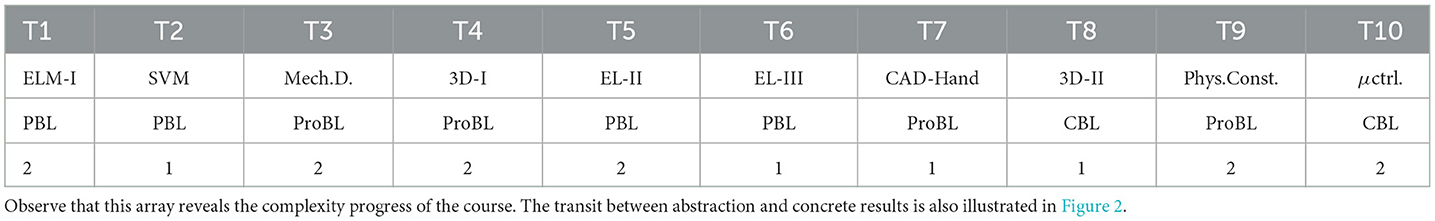
Table 1. Topics, themes, AL techniques used, and duration in weeks are illustrated here.

In the 10th session, the hand had to be presented, working correctly. It should be noted that the development reported in Section 3 is the result of the experience accumulated in the years 2009, 2014, 2021, and 2022. In particular, we were able to mature all this during the continuous period 2021–2022.

3 Materials and methods: SciTSA-AL elements

The organization described in Section 2.2 is resumed in Figure 1 (the meaning of their blocks will be defined in the lines below, but it is resumed in Table 1). As mentioned above, our SciTSA-AL method consists of seven parts. The time needed to implement each of them is indicated in the illustration. Note that this time frame contrasts with the one shown in Table 2, where the course duration is separated by themes and not by SciTSA-AL phases. In that table, we summarize the topics, AL technique, and duration in weeks of each of them. As can be seen, the course consists of 10 themes (T1–T10; more details in Table 1). The 2nd row shows the content of each topic: ELM (Euler-Lagrange modeling phases), SVM (state variables equations), Mech.D (mechanical design stage), 3D (three-dimensional animation in open and closed loop, I, II), and μ-controller unit programming. Below this, the proposed active learning techniques are given (see Section 2.1). Finally, the last row provides the duration (in weeks) by topic.

Figure 1

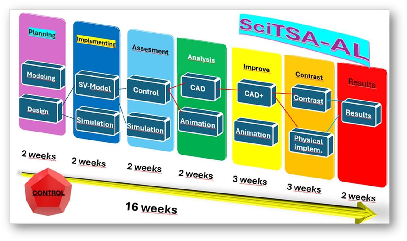
Figure 1. The structure of our SciTSA-AL consists of seven parts as described in Section 2.2. The blue lines that connect planning to assessment stages denote open/closed loop mathematical modeling. The outcomes of this are tested during the assessment phase. In contrast, red lines reveal the 3D computational and physical version of the latter. Finally, blue lines denote the convergence of all this. The dodecahedron emphasizes our conscious desire to truly convey Control Systems and Mechatronics topics to our students.

Table 2

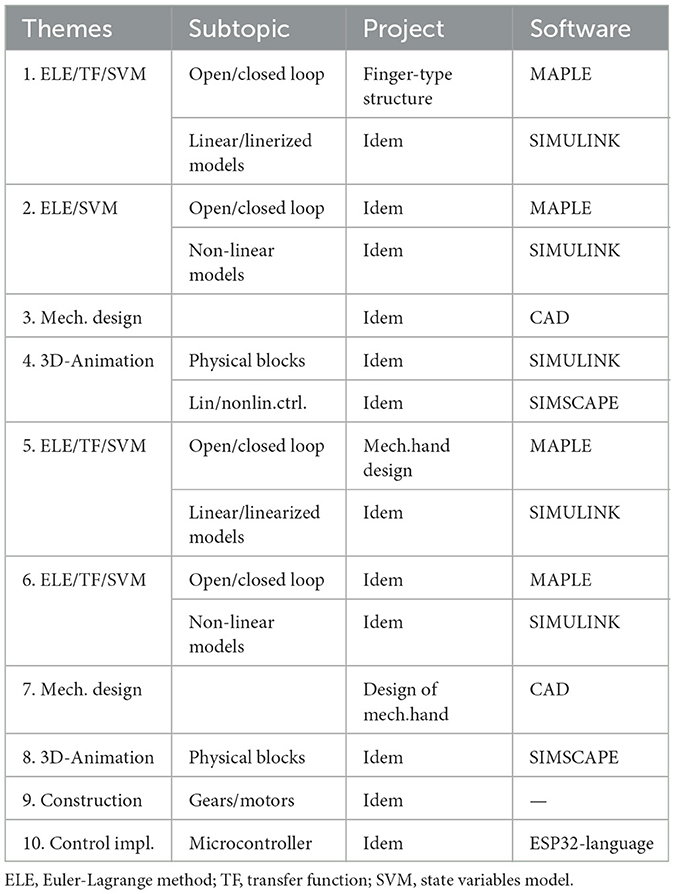
Table 2. Themes, projects, and software used in our SciTSA-AL program.

The study was developed at the Instituto Tecnologico de Monterrey, campus Ciudad de Mexico, and the investigated subject was Laboratorio Integral de Control Automatico (Integral Automatic Control Laboratory). Although the name laboratory would imply a lot of practices with less theoretical activities, this course is intended to encompass advanced control techniques for complex plants as well. That is why the theoretical component is very relevant here; there are many self-contained topics. In addition, the instructor has the liberty to modify the content of the course with respect to the level and the background of the participants. A structural decomposition of our proposal is shown in illustration Figure 2.

Figure 2

Figure 2. SciTSA-AL framework. The progression from mathematical abstractions is gradually performed by the numerical solution of non-linear differential equations that later “animates” 3D-CAD-based models (in open and closed loop). This activity converges to the physical construction of the mechanical hand, controlled by the microcontroller. Thus, computational models in open and closed loops are replicated with real-life implementations.

In this sense, to facilitate the understanding of the proposed study plan, the information is presented as follows:

• Modeling by Euler-Lagrange (EL) equations.²

° Linear models.

° Non-linear models.

• State variables-based models and control.

° (Linear) state variable models and state feedback.

° (Non-linear) state variable models and state feedback.

• Implementation of the control law in a microcontroller unit.

• Development of a complex mechanical structure.

° Mechanical finger (linear and nonlinear) model.

° Creation of a CAD model of a single two-degree-of-freedom finger.

° Importation of the CAD model from SIMSCAPE.

° 3D animation (open loop and closed loop by PID controller).

• Integration of fingers to a CAD-palm. Design of a CAD-prosthetic hand.

° Importation of these CAD pieces from SIMSCAPE.

° PID control of fingers in the hand.

° State feedback to control fingers in a particular sequence.

• Physical construction of a finger. Replication to form a hand.

° Control implementation in a microcontroller unit.

The previous arrangement is organized and complemented in Table 2, where 10 projects can be easily identified.

As remarked, the application of specialized software, such as MAPLE (symbolic calculations), MATLAB, SIMULINK (scripts and block systems), and SIMSCAPE (physical blocks with 3D animations), was essential for math modeling and control theory. Notice that in 2022b, the hardware part was included. Nevertheless, not all of this was always at hand (see Table 3). There, G means group, SMLK means SIMULINK, and SMC means SIMSCAPE. V1 indicates a video produced to show a 3D animation (SIMSCAPE) working adequately. Prod designates a software (S) or hardware (H) creation. V2 means that the activation of a device was filmed.

Table 3

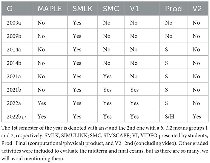
Table 3. Software used by semester.

We now proceed to briefly present the main characteristics of the class project as well as its objectives. Besides, each of the 10 topics is explained with its respective outcomes. The AL technique utilized was also added. These activities will converge in the actual construction of the controlled mechanical hand.

3.1 AL-techniques by theme in SciTSA-AL environment

Main project. Modeling, simulation, and implementation of a controlled mechanical hand (CBL; Queen's Univeristy, 2023). The steps of CBL were done along the whole course and were decomposed and mixed with the typical AL methods identified as useful for us in Section 2.1.

Requirements: Differential equations, Continuous Control Systems, Digital Control, Electronics, Mechanics, CAD.

Goals: At the end of the course, the student will be able to

• Apply the EL-method to represent electromechanical systems.

• Develop complex symbolic calculations for modeling in specialized software.

• Perform 3D animations of open/closed loop systems in technical software.

• Develop a physical implementation of an electromechanical device represented by 3D animations.

• Perform a control design implementation via a microcontroller unit.

Comments: The mechanical hand is a real-world application. Intense interaction among students is desirable and necessary. The students will work in teams of 3–4 people as our Labarotory requires. The goals given above will be acquired by means of scientific and technical software support. In addition, the physical construction of a prototype will close the SciTSA-AL process.

Assignments and goals by topic:

Theme 1. EL-modeling (PBL; Cornell University, 2023). The EL method for modeling is taught and compared to other modeling techniques. PBL was used because we gave students a prompting problem to investigate: a mechanical structure of a knuckle and a phalange (half finger).

Goal: Modeling with EL equations of a mechanical half finger. Equivalence of EL equations and state variables/transfer functions (SV/TF) is performed. Use of symbolic calculation software (MAPLE) is key. See Figure 3.

Figure 3

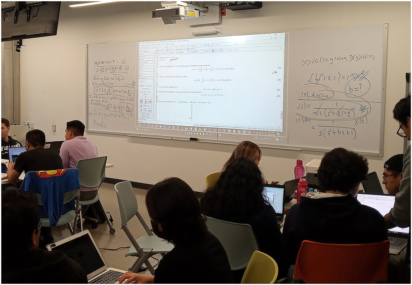
Figure 3. The students developed mathematical models by hand and compared them with the results provided by MAPLE (projected on the whiteboard).

Outcome: Modeling/control of linear and linearized models of a mechanical knuckle-phalange in MAPLE.

Theme 2. EL-equations/state variables models (PBL; Cornell University, 2023). In line with PBL, we present participants with the real effects of a problem. The half-finger model presents non-negligible non-linearities. Students learn the equivalence between EL equations and non-linear state variable systems. Moreover, by replication of a single knuckle-phalange array, a complete finger can be defined.

Goal: Identifying suitable analytical representations for linear and non-linear systems in terms of EL equations and state variable models.

Outcome: Open/closed loop non-linear knuckle-phalange/finger model.

Theme 3. Mechanical design of a complete finger in CAD (ProBL; Boston University, 2023). Similarly to theme 2, a complete finger is assembled here. Critical thinking, teamwork, and conflicting design ideas were key.

Goal: Constructing a finger structure in CAD software.

Outcome: A CAD file of a mechanical finger is developed. Later, replications of this initial finger will be performed to form a hand.

Theme 4. 3D animation (open/closed loop) and ProBL (Boston University, 2023). CAD (Autodesk Fusion 360) was used to create a mechanical finger composed of two phalanges and two knuckles. Importation of CAD files from SIMSCAPE was taught. SIMSCAPE-based models are compared with TF/state variables representations. Participants were challenged to create a computationally controlled mechanical finger prototype that could be moved properly.

Goal: Realization of 3D animations in SIMSCAPE imported from Autodesk Fusion 360.

Outcome: An animated full finger SIMSCAPE model (with/without controller). A video of the animation plus a detailed report is also presented. Questions were asked from one team to the other.

Theme 5. EL method to model a complete mechanical hand linear model (PBL; Cornell University, 2023). The experience of modeling a single finger is generalized to a group of them attached to a palm to create a hand. A linear controller is also implemented.

Goal: Identifying a modeling pattern from one finger to repeat it for a set of them. The control action is designed in SIMULINK. Equivalences among ELE, TF, and SVS are obtained.

Outcome: SIMULINK file with open/closed loop responses.

Theme 6. ELM to model the hand (PBL) in non-linear version. In PBL, students must deal with a real problem where each participant has to acquire knowledge. Discussions take place keeping focus on the process, leaving the final solution to the end.

Goal: From ELM, a non-linear state variable model is deduced for the hand. Later, a non-linear controller is designed.

Outcome: (Uncoupled) non-linear open/closed loop models are obtained in MAPLE and SIMULINK.

Theme 7. Mechanical CAD of a hand (ProBL). This case is an inductive reasoning from Theme 3. See Figure 4.

Figure 4

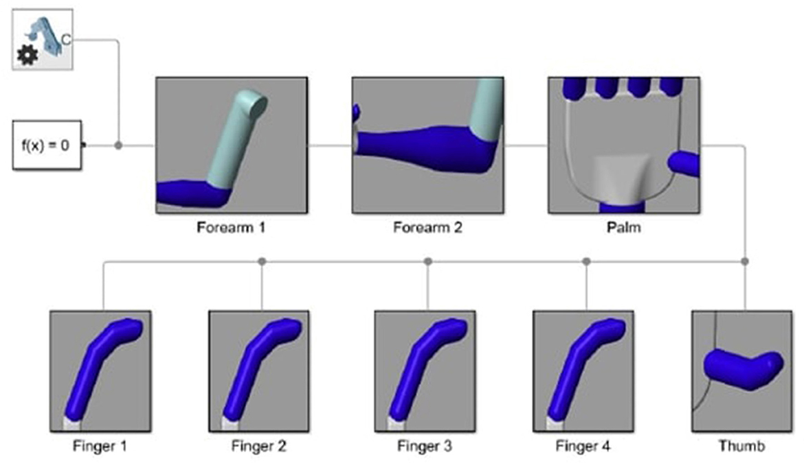
Figure 4. A high-level masked block diagram of the controlled hand is shown here. This set of eight SIMSCAPE-SIMULINK blocks makes up the computational model (open/closed loop). Many details of each building block are hidden by representative images of each part of the hand. The idea of replication modeling and synthesis was actually grasped after showing the students that replicating a finger on a palm defines a hand. However, a “big finger” (arm+forearm) also constitutes a higher structure in the same sense (theme 7).

Theme 8. 3D animations of the uncontrolled and controlled hand (CBL). CBL was implemented to enhance past experiences, but is now using SIMSCAPE software. The case study of designing a completely controlled mechanical hand with 3D animations is given. This part is induced during discussions and comparisons, remembering the beginning of the project with a single phalange. See Figures 4–6.

Figure 5

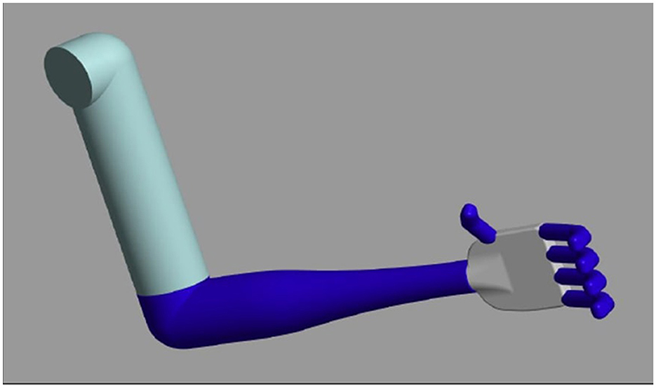
Figure 5. After finishing the design of the hand (Figure 4), a higher level structure is computationally built (arm + forearm, theme 8).

Figure 6

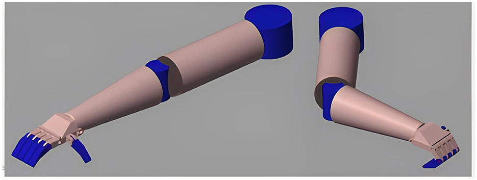
Figure 6. Another example of an arm and forearm that follows the hand design (Figure 4). In this case, the animation starts with an extended arm and ends with a bent arm (bottom right).

Goal: Designing suitable control laws to govern the complete hand, finger by finger, using physical blocks in SIMSCAPE.

Outcome: A fully animated and controlled SIMSCAPE model that moves correctly following a complex reference signal is produced. The file is enriched with a video and a detailed report.

Theme 9. Physical construction of the hand (ProBL). This is the culmination of all the previous phases. Clearly, students have to work as a team, they have to plan, design, and implement (Figure 7).³

Figure 7

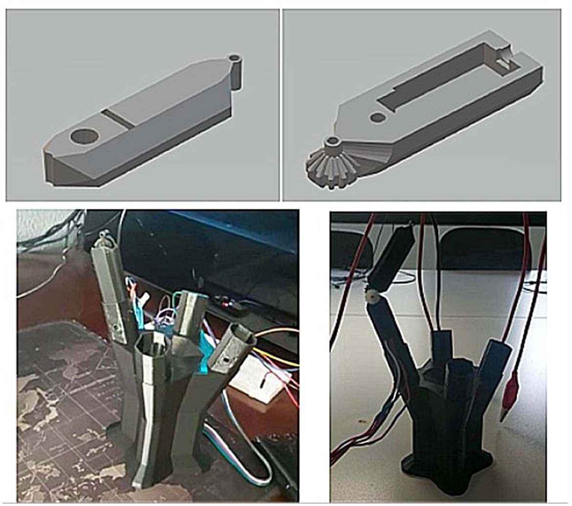
Figure 7. An example of a robotic hand construction. Left upper panel: CAD design of a lower phalange. Right upper panel: upper phalange. Below: hand base and a lower phalange. Next to it, a complete finger was installed. All these components were 3D-printed.

Goal: Organizing and designing a physical prototype of a robotic hand based on modeling, numerical simulations, and 3D animations as an open-loop system.

Outcome: Implementation of a robotic hand working in open loop. Structure produced by 3D-printing (Figure 7).

Theme 10. Implementation of a control law in a microcontroller unit (CBL). Finally, once the robotic hand is built, it is time to implement a control law. Since the hand is finished, we considered it convenient to apply CBL because the hand is the case study (Figure 8).

Figure 8

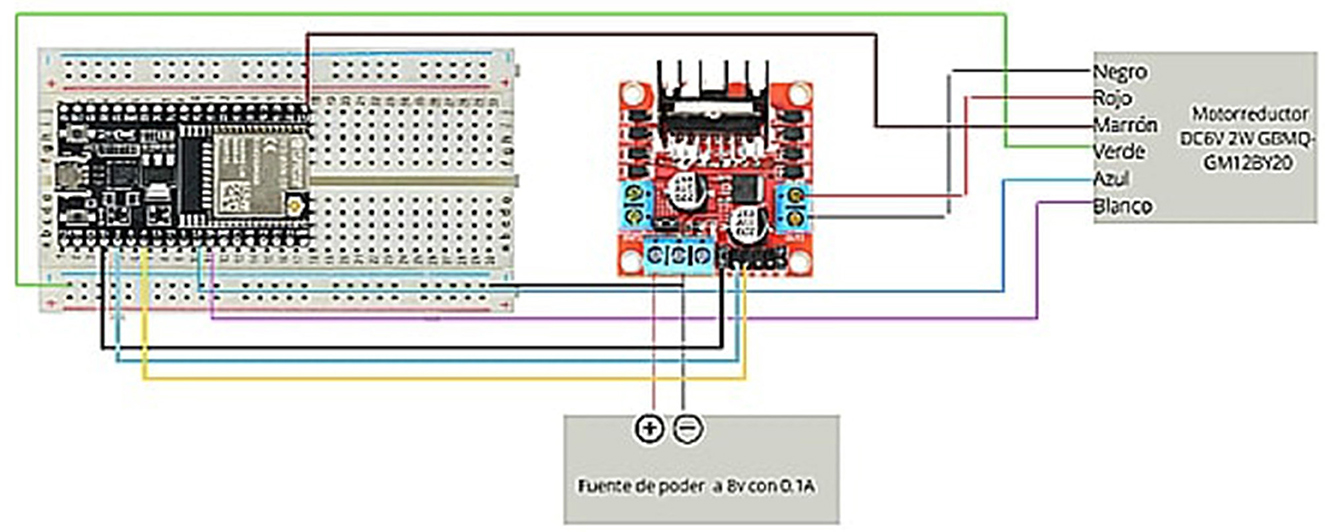
Figure 8. An example of a microcontroller unit on a breadboard that will activate and control the robotic hand.

Goal: Selecting a suitable and reliable microcontroller unit for the previously designed robotic hand. Programming a PID control in the microcontroller. See Figure 9.

Figure 9

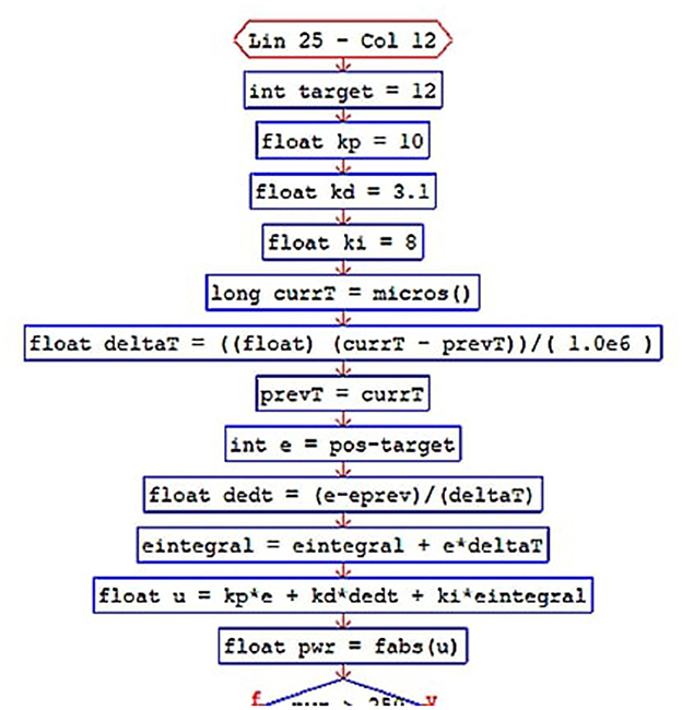
Figure 9. Detailed flowchart of the ESP32 language to program a PID control. With this image, we wish to emphasize that during math analysis, coumputational implementation, and microcontroller-based programming, the structure of a PID control remains the same.

4 Results

As can be seen, the construction of the hand started from a simple model based on a pendulum to define a mechanical phalange. From this, the work was extrapolated to a finger, then to a collection of them, and finally this set was mounted on a palm. This process was a combination of analytical-computational work that generated a 3D animation of the controlled structure. In this spirit, beyond that, two physical results were presented, a real robotic hand and the implementation of the controller. Obviously, the good behavior of the physically controlled mechanical hand was already a proof of the success of the students. To complement these physical results, we will now analyze the grades of the students collected during the semester. Thus, the set of two exams by stage together with their corresponding project (10 as observed above) defined a record for each student.⁴ These activities were developed during the 16 weeks that the course lasts. We then statistically tested the difference in the mean of those exams against the corresponding project. These results confirmed that our strategy succeeded.

4.1 Statistical analysis

As it was already mentioned, we suddenly detected background problems in our Mechatronics students. Our administration took care of these groups in discontinuous periods: 2009, 2014, 2021, and 2022. Since this situation was identified in 2009, that was the year we started a new organization of the course, which evolved until 2022. In that year, we particularly noticed great progress in our students. The outcome of that synergy was the construction of the controlled mechanical hand.⁵ The results of this section allowed us to objectively verify the qualitative achievements obtained via our SciTSA-AL. In this context, a simple observation of the final averages and coefficients of variation by group (Table 4) gave us an early feeling of confidence. The cvs display an oscillating upward trend, may be an adaptation effect.

Table 4

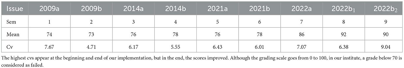
Table 4. Final grades by group and coefficients of variation (cvs).

A deeper comprehension of our planning results will be obtained by comparison of exam and project grades. In our organization, each project grade P also implied two exams (with average X). We considered a key issue to investigate the difference Δ between P and X, i.e., Δ_i = P_i − X_i, i = 1, …10 (see Section 3.1). Thus, a student record was composed by one project and two exams (by group). The descriptive statistics of Δ are shown in Table 5 by group. There, n is the number of students by class, Min and Max are minimum and maximum of Δ, respectively. “Av” is the mean and q₁, q₂, and “Iqr” are the first quartile, second quartile, and the interquartile ranks, respectively. Actually, Δ_{i, j, k} = P_{i, j, k} − X_{i, j, k} for i = 1…p, j = 1, …n_k, k = 1, …, g, for p = 10 projects, n_k is the number of participants by class and g = 9 groups. From that table, we can notice that the highest medians were obtained in 2021, a period after which our institute was rebuilt (earthquake 2017) and the pandemic began to stabilize. Interesting too is the comparison of 2009 (poor condition of students) and 2022 (hand project). Actually, eight out of nine classes had positive medians (improvement via projects).⁶

Table 5

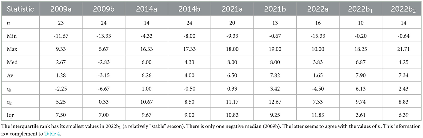
Table 5. Descriptive statistics of Δ.

In line with this, we wanted to determine if there was a significant change in the nine groups considering the grades of the exams versus each corresponding project by participant. Our institute considers a number of students enrolled between (15,35)⁷ per class per semester. This means that we have small sample sizes. Additionally, the normality of data was assessed. For this, a Shapiro-Wilk test showed that our data did not behave normally at a level of 5 %. These facts guided us to conduct a non-parametric study (Dekking et al., 2005; Martinez-Gonzalez, 2020). Since the associated probability distributions resulted to be non-normal, we have groups of less than 50 students, and we want to objectively compare groups between them, we use the Wilcoxon signed test (WST) and the Wilcoxon rank sum test (WRST) (Martinez-Gonzalez, 2020; Pallant, 2016; Tomczak and Tomczak, 2014).

Accordingly, this procedure was executed in two phases: an “internal” one (comparing partial grades versus projects per class) and an “external” one (contrasting 3 pairs of groups between them). Therefore, we have the following:

Stages:

• Δ was computed for each group and for each participant. From this, a Wilcoxon signed test (WST) was utilized to determine whether the median of a population is significantly different from zero.

• A two-sample Wilcoxon rank sum test (WRST) is performed to compare results obtained during key moments. Therefore, we decided to evaluate 2009a vs. 2021a; 2021a vs 2022b; and 2009a vs. 2022b. Thus, the contrast was done comparing the results obtained during the beginning of our solution against a middle development; again, this stage versus the time at which the hand was built, and from the very beginning with the final phase. This means testing Δ₁ vs. Δ₅, Δ₅ vs. Δ₉, and Δ₁ vs. Δ₉ to discover if improvements (if any) were significantly distinct.

Outcomes:

• The WST produced Table 6. This procedure tests the null hypothesis that the data in Δ come from a distribution whose median is zero at the 5% level. From the table, seven out of nine classes show a logical value of h = 1 (true). This indicates that the test rejects the null hypothesis of zero median at the 5% level. With that confidence, there appears to be an optimistic effect of the projects. Remember that, traditionally, this course did not have this kind of activity. This is not the case for 2009a and 2022a (semesters 1 and 7, resp.).

• Now we want to know if the measures of improvement in all classes were significantly different. Before proceeding with the application of the WRST, a box plot is presented in Figure 10 for each Δ. We already know that notches typically do not overlap if median values are significantly different from each other at the 5% level. From that picture, we observe that notches do not overlap (excluding semesters of 2021 and 2014b with 2022b1). If two notches do not overlap, it means that their medians are significantly different. The case of groups of 2022 is special because of the flipped aspect. The reason why notches extend beyond the 25th and/or 75th percentiles is due to the uncertainty of the true median value. This occurs if a sample size is relatively small (Dekking et al., 2005; Martinez-Gonzalez, 2020).

Table 6

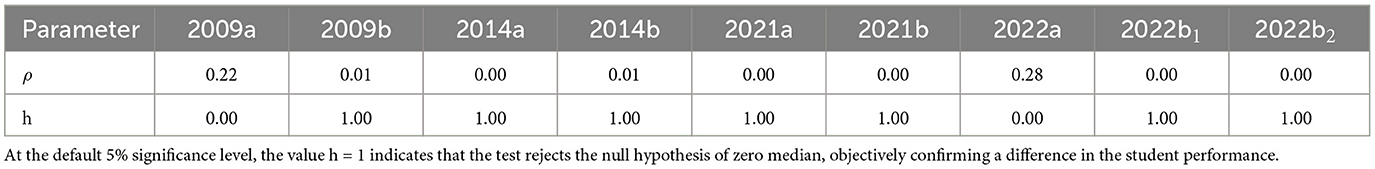
Table 6. WST.

Figure 10

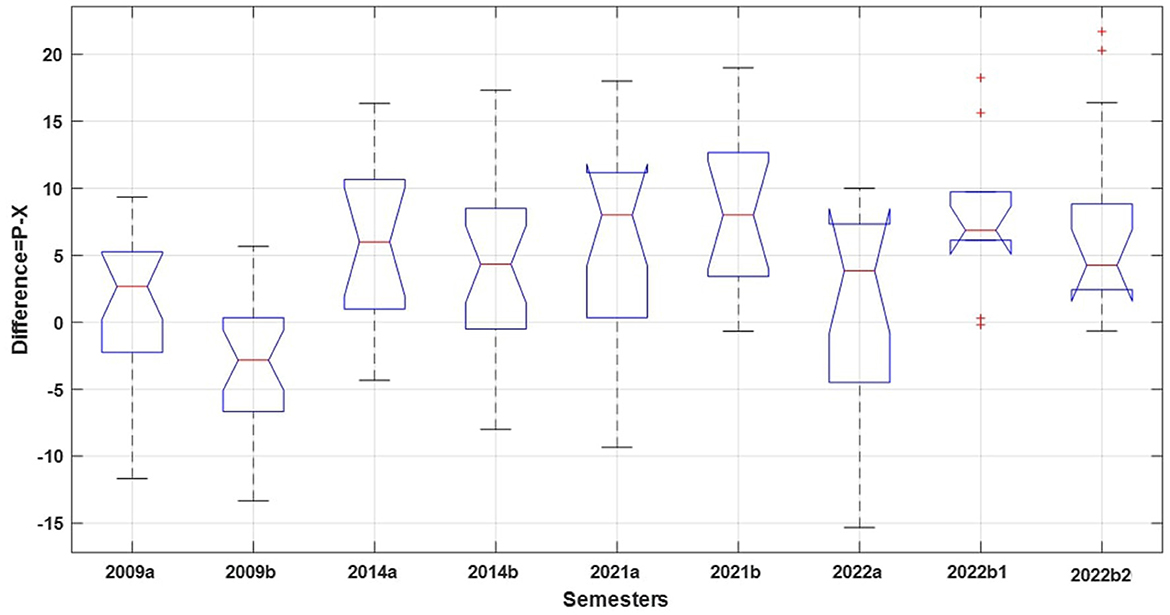
Figure 10. Box plots for Δ. Data are quite scattered in the middle periods and less so at the end. However, in 2022, groups presented outliers, which may be a result of team and individual work to build the mechanical hand.

Next, a formal WRST test tests the null hypothesis that data in two collections are samples with equal medians, against the alternative that they are not with significance at the 5% level. Outcomes of this part are given in Table 7.

Table 7

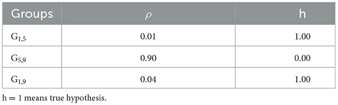
Table 7. WRST to compare groups 1,5,9.

The values of ρ < 0.05 and h=1 denote the rejection of the null hypothesis of equal medians at the default 5% significance level. Therefore, significant differences from zero are perceived in cases 1 vs. 5 and 1 vs. 9. Therefore, students of group 1 seemed to have learned a little more between exams and project than the students of groups 5 (2021a) and 9 (2022b2). This fact seems to suggest that an actual improvement (via projects) occurred from the detection of the problem (2009a) to the middle periods (2021a) and from that detection to the final period. This is not the case for middle times (5) to end epochs (9), where both the ρ-value and h = 0 indicate that there is not enough evidence to reject the null hypothesis. This fact seems to indicate that students did not learn more from the exam period to the project time. Finally, it is worth considering whether improvements in key groups medians have any practical significance. This issue is explored next.

4.1.1 Calculation of effect size (side effect)

It is well known that in conjunction of ρ, the size of the observed effect must be included. This effect of size will allow us to know if, besides being significant, the difference is practical. The effect size for a Mann-Whitney-Wilcoxon test (MWWT) or a WSRT (Pallant, 2016) is commonly determined via a correlation coefficent in terms of the standarized z-score with $r_{RCC}=z/\sqrt{n}$, where n is the total number of samples of all records, i.e., n = n₁+⋯+n_g for g, the number of groups This quantity is some times referred to as the Rosenthal correlation coefficient (RCC; Rosenthal, 1994). Despite its simplicity, it has some drawbacks. The biggest of them is that r_RCC sensitive to the size of n, i.e., to each n₁, …, n_g. Contrastingly, the rank biserial correlation coefficient (RBC)⁸ is chosen to report effect size estimates in Wilcoxon tests. This coefficient helps us see how items or subjects in one group are ranked compared to a second group. It indicates the discrepancy between the portion of ranks in favor of or against the hypothesis (Dekking et al., 2005; Martinez-Gonzalez, 2020; Rosenthal, 1994; Pallant, 2016). Accordingly, r_RBC is defined as (Tomczak and Tomczak, 2014):

$\begin{array}{cc}{r}_{RBC}=\frac{4\left[T-\left(\frac{R_1+R_2}{2}\right)\right]}{n(n+1)}& (1)\end{array}$

Where, T = min(R₁, R₂), R₁, sum of ranks with positive signs; R₂ sum of ranks with negative signs; n, total sample size. The outcomes of these tests were obtained in MATLAB and are summarized in Table 8 (Cohen, 1988).

Table 8

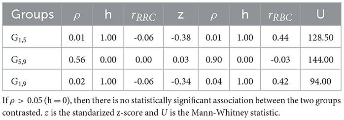
Table 8. Effect size via r_RRC (green section) and via r_RBC (blue part).

Table 8 reflects that parameters ρ and h coincide, expressing rejection of the null hypothesis of equal medians at the default 5% significance level for pairs G_{1, 5} and G_{1, 9}. For G_{5, 9}, ρ and h suggest that there is not enough evidence to reject the null hypothesis. Nonetheless, |r_RRC|≪|r_RBC| and their signs are inverted, suggesting contrary effects. Analyzing r_RRC, we deduce that there is a very small deterioration in group 1 compared to a small improvement in groups 5 and 9, and the other way around. However, since r_RRC ≈ 0 and by the reasons given above, it is more convenient to consider r_RBC as an effect size indicator.

Depending on the values of r_RRC and r_RBC, a scale of relation between two groups is defined in Table 9 (Bartz, 1999; Cohen, 1988; Kerby, 2014).

Table 9

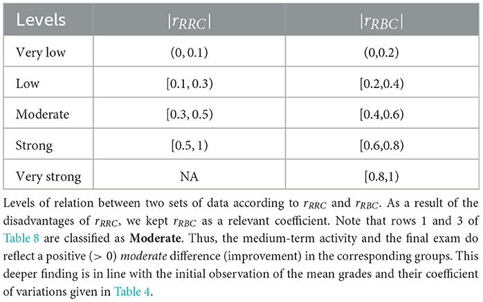
Table 9. Common language effect size.

Recall that the effect size indicates the significance of the relationship between variables or the difference between groups. It reveals the realistic relevance of a research result. A large effect size means that a research finding has sensible relevance, while a small effect size indicates limited feasible applications. Table 9 permits the objective expression in common language of what Table 8 communicates in terms of the null hypothesis. Thus, from both sides of the table, we can finally conclude that we reject the null hypothesis of equal medians at 5% of significance in groups 1 vs. 5, on the one hand, and in groups 1 vs. 9, on the other. Median of Δ in groups 1 and 5 are 2.67 and 8, respctively. Hence, a difference of 8 − 2.67 = 5.33 represents a moderate improvement, of class 5 vs. class 1. The same happens with groups 1 and 9, where D is 4.25 − 2.67 = 1.58.

Now, in the case of classes 5 and 9, there is not enough evidence to reject the null hypothesis of equal medians. Here, D = 8 − 4.25 = 3.75 reveals a low improvement of group 5 with respect to 9. In spite of this apparent achievement of group 5, we must remember that these students presented the highest variation in the entire study.

5 A glance at student's opinion

Although the last section has objectively shown the statistical reliability of our method, we would like to share a brief comment about students perceptions via the end-of-course survey. In Figure 11, part of the complete evaluation by group is given. On top, we can read “Sistema de encuestas” (Survey system) and below it, “Reporte de comentarios” (Comments report). In the table, the first column indicates the campus where the class was taught. The second column shows the subject code. The third and fourth elements provide the course name (Process Automation Lab) and group number, respectively. Columns five and six report the number of students expected to graduate and the number of people who provided opinions on the topic. At the end, students' comments are directly shown. The four opinions shown in the table are positive; however, the third one says that: “It would have been great if we could have worked at the lab and not only with MATLAB”. We highlight that students generically call MATLAB the binomial MATLAB-SIMULINK, and if we review the Table 3 again, what this person says makes sense.

Figure 11

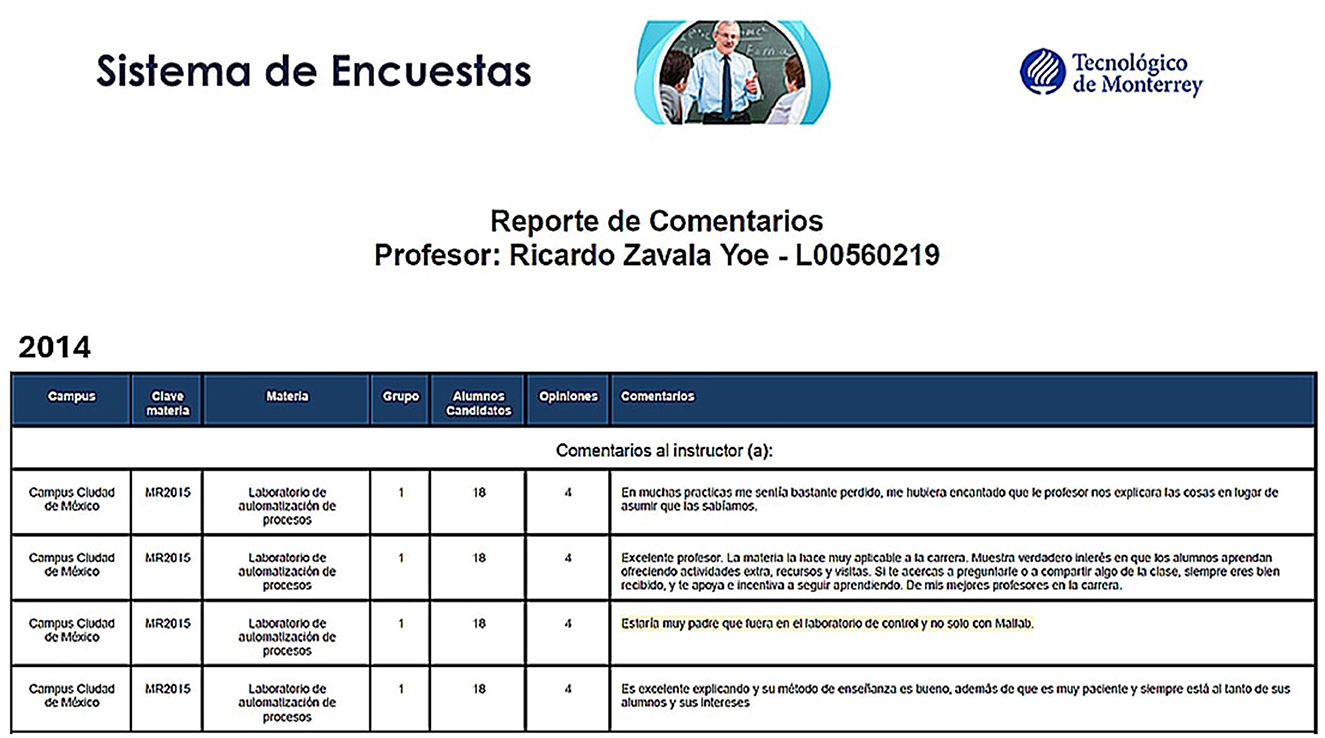
Figure 11. A sample of an en-of-course survey (2014). In the 3rd row, a student says that: “It would have been great if we could have worked at the lab and not only with MATLAB”. Our perception (as teachers) was also in line with student's remarks, and that is why we proposed the innovative method described in this work. MATLAB-SIMULINK, although good, was not enough.

Figure 12 (topmost panel, 2014) reflects the perspective of other students enrolled in another class (Process Automation). What is relevant here is the second viewpoint. This student states that: “The teaching style is questionable but (the professor) is fair in grading. I wish we had had computer activities”. Although computational activities were definitely present, the student may complain about having worked more with SIMULINK than with MATLAB (“block programming”). This perspective is, in some sense, contrary to the one given above, where the person mentions that he/she had a lot to program in MATLAB (besides the lack of manual events). Now, it is interesting to read what another student thinks about the same course but followed in 2021a (after the 2017 earthquake and still during 2020–2021 COVID pandemic). This person says that: “Excellent professor, he could adapt to the hybrid (teaching) model and giving a class with academic quality via Zoom. The classes were very clear and he solved all my doubts, he uploaded a lot of material to Blackboard, for instance, exercises to complement the class”. This student is satisfied with our new implementations despite working in remote mode. As a complement, another viewpoint is given in 2021b where the person expresses that “He (the teacher) is very patient and he solves our your doubts, it does not matter how many times you ask him. He really cares about teaching us. Although we find it difficult to learn on Zoom, he works hard when it comes to teaching and continues to go further :) (happy face, i.e., satisfaction). If for some reason you get low grades it is because of Zoom, it is very difficult to concentrate on the screen (in remote learning we had to spend a lot of time teaching-learning via Zoom)”. In this case, the student does not complain about the computational resources, nor about the manual activities, but about the mandatory nature of distance learning. Finally, in the last row, a student says that “He (the teacher) is very friendly and that is why some times the class may be disordered. At some moments, he teaches a lot of theory and uses MAPLE a lot and I personally think that this time should be used in practice exercises”. Here, the student is happy with the professor performance and attitude but complains about some “induced” disorder (as a result of the necessity of using Zoom the whole day) and the exigency of using MAPLE to “replace” close personal explanations. This comment is also interesting because this person recognizes the teacher's effort, but at the same time accepts the implicit disadvantages of long periods of remote learning. Obviously, practical exercises were definitely not possible during the COVID-19 pandemic, and that is why the practicals had to be done through software. Besides, the student does not protest (directly) against software, active learning techniques, but rather against implicit long-time sitting in front of the computer screen. We must remember that everyone at our institution was tired of remote learning and home office also due to the time we were waiting to be assigned to some improvised facility after the 2017 earthquake.

Figure 12

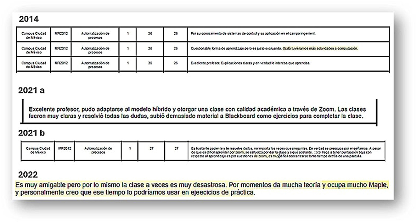
Figure 12. Opinions of students about the progress of our adaptive learning process. The 2022 comments also correspond to the Automation Processes class.

Finally, in contrast to the observations given above, 2022b improved a lot (see Figure 13). Although we only offer a sample of a survey, most of the comments did not show serious complaints. It is important to note that during the study period, in general, the teacher was well evaluated by the students. However, as we can see in our study, student complaints decreased as our new method was implemented. What was nearly impossible to reduce were complaints about prolonged use of Zoom due to the need for remote learning. It is also worth noting that from observing Figure 13, there appears to be a combination of the teacher's attitude and the progress of our SciTSA method. The first row says: “Very good teacher. He knows a lot and make the class dynamic”. Second row: “He is an excellent teacher, he domains the topics, he is very patient to explain what you can not understand, he is always open to mentoring. He cares about your understanding.” And the 3rd row closes saying that: “He is an expert on the theme, he creates a pleasant and reliable work environment, although the home works were long and complex.”

Figure 13

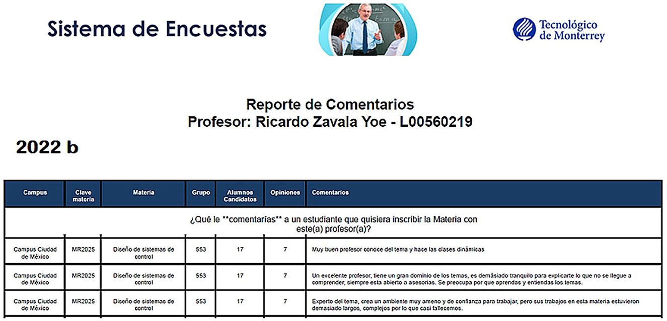
Figure 13. Final year of our implementation. Notice that the type of complaints (at least in this sample) is not related to software, remote learning, etc., but with the implicit difficulties of the course.

6 Discussion

As it was established from the beginning of this study, the idea of this study was to explore new ways to reliably grasp the content of Mechatronics suitably. As a result of not identifying a suitable bibliographical reference that could have helped us, we developed our own AL technique, referred to as SciTSA-AL. This process implied a redesign of the course with a fine and close supervision of the students. They were motivated by the modeling and design of a robotic hand. The steps to construct the main project were implemented by 10 intermediate activities (complemented with two exams by outcome). Although the robotic hand was constructed correctly, and final marks improved, a statistical analysis verified our observations. Now we can claim that we are 95% confident that the introduction of those manual activities was useful in six out of nine groups. We also need to remember that in 2021 (periods 5 and 6), our institute had been recently rebuilt after the 2017 earthquake. In addition, the pandemic was beginning to stabilize, and attendance at the institute was irregular due to activities being conducted remotely via Zoom.

As it was described in Section 1, there are just a few studies that actually address the problem of effective learning of Control Systems in Engineering. In the literature reviewed in that section, we demonstrate that the research carried out there is short-term, whereas ours encompasses several years. Moreover, the examinations described in those references are applicable to particular situations using only one type of software. In contrast, although the investigation offered in Rojas-Palacio et al. (2022) is too general, it does not deal with software support. Furthermore, none of them were carried out for several years, a period in which catastrophic events were recorded that occurred almost consecutively. Thus, the strong point of our study is that we analyzed a set of AL techniques and from them we chose those that we considered most suitable for our courses, taking into account various types of software support that converge in the construction of a real robotic hand. Some unexpected findings were that the teacher has been positively evaluated this entire time as our implementation progressed. Furthermore, student complaints were mainly due to outdated learning processes (which were already changing with our strategy) and some other difficulties inherent to the course, as well as discomfort caused by extremely long periods on Zoom. We consider that our proposal could be extended to similar situations because the profile of our students is comparable to that of others (and even ours!). However, to date, we are not aware of similar studies.

7 Conclusion

We are convinced that the learning path followed in this report solves the problems exposed from the beginning. Early identification of a lack of theoretical understanding is mandatory, and moreover, in courses as these, theoretical understanding allows extending knowledge to the next level, numerical solutions of mathematical models (2D graphics). If apprentices had grasped this part, 3D animations in open and closed loop flows very naturally. If this structure can be embodied in a physical prototype where a microcontroller can govern it, then the cycle closes, endowing students with an actual comprehension. This is what we identified as our SciTSA-AL. It may not be perfect, but it is new and it works.

Data availability statement

The raw data supporting the conclusions of this article will be made available by the authors, without undue reservation.

Ethics statement

Written informed consent for participation was not required from the participants or the participants' legal guardians/next of kin in accordance with the national legislation and institutional requirements because only numerical data was used. The studies were conducted in accordance with the local legislation and institutional requirements.

Author contributions

RZ-Y: Conceptualization, Formal analysis, Resources, Software, Validation, Visualization, Writing – original draft, Writing – review & editing. BU-A: Conceptualization, Investigation, Resources, Supervision, Validation, Writing – original draft. EL-C: Methodology, Validation, Visualization, Writing – review & editing. RR-M: Conceptualization, Supervision, Validation, Writing – original draft.

Funding

The author(s) declare that no financial support was received for the research and/or publication of this article.

Acknowledgments

We are extremely grateful to Carolyn Hill (Maplesoft) for allowing us to use Maple for 2 years, especially during the most disastrous times and when we needed it most.

Conflict of interest

The authors declare that the research was conducted in the absence of any commercial or financial relationships that could be construed as a potential conflict of interest.

Publisher's note

All claims expressed in this article are solely those of the authors and do not necessarily represent those of their affiliated organizations, or those of the publisher, the editors and the reviewers. Any product that may be evaluated in this article, or claim that may be made by its manufacturer, is not guaranteed or endorsed by the publisher.

Footnotes

1. ^The course is 4 hours per week. Of them, two are theoretical and two are practical, without being strict, allowing small variations in the distribution of time. This depends on the topic to be discussed.

2. ^Some other important topics, such as kinematic constraints, some types of DAEs (differential-algebraic equations), etc., are considered here, but we use the generic term Euler-Lagrange models for ease of exposition.

3. ^We must clarify that the computational and physical designs differ a little because there were some logistical problems that we had to suddenly solve on the 3D printer, but since we wanted the students to carry out this stage by themselves, we had to compromise a little about the modifications.

4. ^As mentioned in Table 3 and Figure 10, there were other individual activities such as personal exams, but to keep the explanations brief, we avoided breaking down the grading system in detail.

5. ^Before this complete work, previous stages were created via software and some simple prototypes using CAD.

6. ^Actually, admission exams, prerequisite courses, etc., were modified during and after the disastrous events.

7. ^Indeed, our n∈[13, 24].

8. ^Actually, the number of methods that report effect size measures for Mann-Whitney U-test and Wilcoxon tests are rather scanty (Pallant, 2016; Tomczak and Tomczak, 2014; Glass, 1965).

References

Alvarado, I. (2006). “Active learning of control theory using virtual instrumentation,” in Fourth LACCEI International Latin American and Caribbean Conference for Engineering and Technology (LACCEI-2006) (Mayagaez, Puerto Rico: LACCEI).

Google Scholar

Astrom, K. J. (1995). A SIMNON tutorial (Research Reports TFRT-3176). Lund: Department of Automatic Control, Lund University.

Google Scholar

Autodesk (2023). Auto Desk Fusion 360. Available online at: https://www.autodesk.com/products/fusion-360/personal (Accessed Februaury 09, 2023.).

Google Scholar

Barnes, D. (1989). “Active learning,” in TVEI Support Project (Leeds: Leeds University).

Google Scholar

Bartz, A. E. (1999). “Basic statistical concepts,” in Upper Saddle River, 4th ed. (Upper Saddle River, NJ: Merrill).

Google Scholar

Bernstein, D. S. (2002). What makes some control problems hard? IEEE Control Systems Magazine. IEEE.

Google Scholar

Boston University (2023). Center for Teaching and Learning Web Site. Available online at: https://www.bu.edu/ctl/guides/project-based-learning/ (Accessed February 23, 2023.).

Google Scholar

Cattaneo, K. H. (2017). Telling active learning pedagogies apart: from theory to practice. J. New App. Educ. Res. 6:2. doi: 10.7821/naer.2017.7.237

Crossref Full Text | Google Scholar

Cohen, J. (1988). Statistical Power Analysis for the Behavioral Sciences. New York: Routledge.

Google Scholar

Cornell University (2023). Center of Teaching Innovation, Center of Teaching Innovation Web Site. Available online at: https://teaching.cornell.edu/teaching-resources/engaging-students/problem-based-learning (Accessed March 10, 2023.).

Google Scholar

de la Lengua Espanola, R. A. (2023). Diccionario de la Lengua Espanola. Available online at: https://dle.rae.es/diccionario (Accesed January 25, 2023).

PubMed Abstract | Google Scholar

Dekking, F. M., Kraaikamp, C., Lopuha, H. P., Meester, L. E., and Modern, A. (2005). Introduction to Probability and Statistics. Cham: Springer.

Google Scholar

del Pais Vasco, U. (2023). Derive. Available online at: http://www.upv.es/derive/general.htm (Accessed Februaury 16, 2023.).

Google Scholar

Donnelly, R., and Fitzmaurice, M. (2005). “Collaborative project-based learning and problem-based learning in higher education: a consideration of tutor and student role in learner-focused strategies,” in Emerging Issues in the Practice of University Learning and Teaching, ed. G. O'Neill (Dublin: AISHE/HEA).

Google Scholar

Elmqvist, H. (1972). SIMNON- An Interactive Simulation Program for Nonlinear Systems (PhD thesis, MS Dissertation). Department of Automatic Control, Lund University, Lund, Sweden.

PubMed Abstract | Google Scholar

Escudier, M., and Atkins, T. (2019). A Dictionary of Mechanical Engineering. Oxford: Oxford University Press.

Google Scholar

Freeman, S. (2014). Active learning increases student performance in science, engineering, and mathematics. PNAS. 111:10. doi: 10.1073/pnas.1319030111

PubMed Abstract | Crossref Full Text | Google Scholar

Glass, G. V. (1965). A ranking variable analogue of biserial correlation: Implications for short-cut item analysis. J. Educ. Measurem. 2:1. doi: 10.1111/j.1745-3984.1965.tb00396.x

Crossref Full Text | Google Scholar

Grace, A. C. W. (1991). “SIMULAB, an integrated environment for simulation and control,” in IEEE-American Control Conference (Boston, MA: IEEE).

PubMed Abstract | Google Scholar

Jayaram, S. (2013). “Implementation of active cooperative learning and problem-based learning in an undergraduate control systems course,” in 120th ASEE Annual Conference and Exposition (Atlanta: ASEE).

Google Scholar

Kerby, D. S. (2014). The simple difference formula: an approach to teaching nonparametric correlation. Innovat. Teach. 3:1. doi: 10.2466/11.IT.3.1

PubMed Abstract | Crossref Full Text | Google Scholar

Klahr, D., and Nigam, M. (2004). The equivalence of learning paths in early science instruction: Effects of direct instruction and discovery learning. Psychol. Sci. 15:10. doi: 10.1111/j.0956-7976.2004.00737.x

PubMed Abstract | Crossref Full Text | Google Scholar

Kovecses-Gosi, V. (2018). Cooperative learning in vr environment. Acta Polytechica Hungarica 15:12. doi: 10.12700/APH.15.3.2018.3.12

Crossref Full Text | Google Scholar

Kozar, O. (2010). “Towards better group work: Seeing the difference between cooperation and collaboration,” in English Teaching Forum, Number 48 .

Google Scholar

Lehtovuori, A., Honkala, M., Kettunen, H., and Leppavirta, J. (2013). Promoting active learning in electrical engineering basic studies. iJEP. 3:EDUCON2013. doi: 10.3991/ijep.v3iS3.2653

Crossref Full Text | Google Scholar

MAPLESOFT (2023). Maple. Available online at: https://cn.maplesoft.com/index.aspx (Accesed March 04, 2023.).

Google Scholar

Martinez-Gonzalez, M. A. (2020). Bioestadistica Amigable. London: Elsevier.

Google Scholar

Mathworks, T. (2022). Matlab. Available online at: http://www.upv.es/derive/general.html (Accessed March 07, 2023.).

Google Scholar

Nola, R., Irzik, G., and Philosophy, S. (2006). Education and Culture. Cham: Springer, Science and Business Media.

Google Scholar

Pallant, J. (2016). SPSS Survival Manual. New York, NY: McGraw-Hill-Education.

Google Scholar

Patete, A., and Marquez, R. (2022). Computer animation education online: a tool to teach control systems engineering throughout the covid-19 pandemic. MDPI-Educ. Sci. 12:253. doi: 10.3390/educsci12040253

Crossref Full Text | Google Scholar

Prince, H. (2003). Does active learning work? J. Eng. Educ. 93:3. doi: 10.1002/j.2168-9830.2004.tb00809.x

Crossref Full Text | Google Scholar

Queen's Univeristy (2023). Center for Teaching and Learning, Canada, Case Based Learing Web Page. Available online at: https://www.queensu.ca/ctl/resources/instructional-strategies/case-based-learning (Accessed March 17, 2023).

Google Scholar

Rojas-Palacio, C. V., Arango-Zuluaga, E. I., and Botero-Castro, H. A. (2022). Teaching control theory: a selection of methodology based on learning styles. DYNA 89:222. doi: 10.15446/dyna.v89n222.100547

Crossref Full Text | Google Scholar

Rosenthal, R. (1994). “Parametric measures of effect size,” in The Handbook of Research Synthesis, eds. H. Cooper, and L. V. Hedges (New York: Russell Sage Foundation).

Google Scholar

Shahini, A., and Mohsen, H. (2013). “Use of mobile devices as an interactive learning method in a mechatronics engineeering course: a case study,” in Proceedings of the ASME 2013 International Mechanical Engineering Congress Exposition (California: IMECE2013).

Google Scholar

The University of Manchester (2023). Centre for Excellence in Enquiry-Based Learning. Available online at: http://www.ceebl.manchester.ac.uk/ebl/ (Accessed January 22, 2023.).

PubMed Abstract | Google Scholar

Tomczak, M., and Tomczak, E. (2014). “The need to report effect size estimates revisited: an overview of some recommended measures of effect size,” in Trends in Sport Sciences 1.

PubMed Abstract | Google Scholar

Wolphram (2022). Wolphram Website. Available online at: https://www.wolfram.com/mathematica/ (Accessed March 15, 2023).

Google Scholar

Zavala-Yoe, R. (2008). “Modelling and control of dynamical systems: numerical implementation in a behavioral framework, volume 124,” in Studies in Computational Intelligence (SCI) (Cham: Springer).

Google Scholar

Zavala-Yoe, R., and Ramirez-Mendoza, R. A. (2019). EEG acquisition and analysis to improve stochastic processes and signal processing understanding in engineering students: refining active learning dynamics via interactive approach in teaching. Int. J. Interact. Design Manuf. 13:7. doi: 10.1007/s12008-019-00601-7

Crossref Full Text | Google Scholar

Zavala-Yoe, R., Ramirez-Mendoza, R. A., and Morales-Menendez, R. (2016). Real time acquisition and processing of massive electro- encephalographic signals for modeling by nonlinear statistics. Int. J. Interact. Design Manufact. 11:2. doi: 10.1007/s12008-016-0366-8

Crossref Full Text | Google Scholar

Ziemann, I., Morari, M., Matni, N., and Pappas, G. J. (2022). Learning to control linear systems can be hard. arXiv:2205. doi: 10.48550/arXiv.2205.14035

Crossref Full Text | Google Scholar