Process automation in biotechnology engineering: reshaping and assessing active learning during disastrous events

Courses such as process automation (PA) can be difficult to grasp, even for engineering students. In addition to the inherent challenge of relating abstractions to real-life situations, we found that our students could not grasp basic concepts. After 5 years of work, we improved our students' performance in these fields. The solution involved redefining the course topics and closely monitoring their learning from the beginning of the course. The approach was enhanced with the support of specialized software and modifications to traditional active learning (AL) methods. Additionally, remote-mode AL was enabled by our institution in response to the 2017 earthquake and the 2019 pandemic. We investigated the difference δ = F−X between projects grades F and exams X via their medians. First, a test was applied to see whether the medians of δ were significantly different from 0. This result was true at 5% of level in 9 out of 12 classes, indicating improvement via F. Later, key groups 2015, 2017 and 2020 were similarly contrasted. Significant differences to zero were appreciated in groups 2015 vs. 2017, 2015 vs. 2020 (progress) but not in 2017 vs. 2020 may be due to those terrible events. Our novelty resulted statistically significant.

1 Introduction

Our process automation (PA) course has had a peculiar history at our institution. This is not only because it is a subject that undoubtedly requires a strong background in various fields but also because of the challenges we faced on our campus. First, the 2017 earthquake forced the rebuilding of the entire institute. Subsequently, the pandemic that broke out in 2019 forced us to perform work in the office and teach remotely. Thus, the period in which we worked on this issue, 2015–2020, was seriously affected by exogenous circumstances. Obviously, our course was not the only one affected, but all our careers' programs were. Remote activities for administration and teaching had to be developed because traditional face-to-face interactions became ineffective. Additionally, new active learning techniques were developed to complement this (de Monterrey, 2019). We would like to emphasize that this research is the result of a retrospective analysis of all these events, spanning from the moment we met these students for the first time during the first semester of 2015 to 2020.

In 2015, we suddenly realized that our traditional active learning techniques had to be improved. From that moment on, we had to work hard to improve the situation. This process has continually matured and was not planned in advance. Rather, we wish to share the results of a progressive event that we unexpectedly encountered. Process Automation is a subject that is taught to our Biotechnology Engineering (BE) students during their 8th or 9th semester.

The BE program has two main concentrations: bioprocesses (BP) and molecular biology (MB). As expected, people enrolled in the BP area are more akin to the PA course, while MB participants considered PA to be a distant affair. Normally, in PA, we have 50% of students enrolled in MB and 50% in BP. We had to face these situations from 2015 to 2020, during which time we identified the following main difficulties in the learning process:

• Teaching PA to apprentices not enrolled in the BP area became even more challenging.

• We had to adapt and rebuild the original PA plan to accommodate remote work (work from home, WFH).

• The latter implied a redefinition and readjustment of the learning methods that we had previously employed.

• Poor background to face this course (aggravated by the tragic events of 2017 and 2019).

The solutions we found to deal with the issues mentioned above were as follows:

• To motivate MB students, we incorporated real-life problems related to their area, such as time-space bacterial growth, tumor evolution, fungus dispersion, and so on. We had to deal with some basic partial differential equations (PDE) theory for this.

• WFH implied a lot of effort done by oneself; thus, support from specialized computer packages was key.

• Redefinition of “traditional” learning techniques forced us to explore and incorporate new active learning (AL) styles (we were fighting against time as well).

• In order to strengthen the students training, a scrutinized monitoring was incorporated from the first day of class but supported by specialized software.

Considering our constraints and the proposed solutions, we attempted to find a report that could have incorporated the remedies proposed above within a single course. As far as we are concerned, there is no literature on the subject, not even a separate study. For instance, upon reviewing reports, we found an AL experience teaching partial differential equations (PDEs) to 3rd-year students in (Cano et al. 2015). However, while the computational tool appears to be useful, students must pay attention to proper coding and numerical issues. From our perspective, those are topics that were studied elsewhere, and for us, that method is not useful. Nevertheless, some other documents also follow this line (Myers et al., 2008; Alfonseca et al., 2002). In this sense, attempting to find a link between theory and applications of PDEs, in (Felse 2018), a particular learning technique is implemented to teach Fluid Mechanics. Although the authors focus largely on fulfilling the course program and how to effectively transmit concepts, they do not consider software issues.

Turning now to lumped systems, (Lozada et al. 2021) covers a wide variety of methods for teaching ordinary differential equations (ODE). This report is quite descriptive and generic, but as such, it does not deal directly with software support. Attempting to find ODE-based applications, typical ODE-based bio-systems are described in (Keener and Sneyd 2009). Although the text is well-explained, software assistance is overlooked.

Now, we will discuss some literature about teaching modeling and control of bioprocesses (to consider our BP concentration). In this area, we found more reports than in math for some biotechnology subjects. For example, in (Rodriguez et al. 2018), a complete description of a collection of AL methods is offered to teach process control. Besides, tailor-made software is used to support the lessons. In contrast, (Ballesteros-Martin and Moral-Rama 2014) implements only Problem-Based Learning (PBL) to improve students comprehension. Furthermore, authors use only one software for simulation and report good results. The perspective changes in (Alam and Zakaria 2021), where a hardware-software combination enables the development of control activities for an actual bioreactor. This is achieved through Cooperative Learning (CooL), which the authors claim improved comprehension and grades.

In contrast to local applications, an Internet-based case is reported in (Hough et al. 2002) where a website was designed incorporating AL activities for undergraduate process control education. In addition to quizzes, simulations, and tutorials, students also have access to a textbook for solving assignments and homework.

The above-mentioned cases were tailor-made for specific situations but unrelated to our events. That is why we had to take specific actions to address our problems. Our main idea was to implement AL plus appropriate software. More specifically, for the mathematical background, we found it very useful to use MAPLE (Soft, 2022; Zavala-Yoe et al., 2019). Through symbolic calculations and graphical user interfaces (GUIs), our students were able to grasp abstract concepts. Lumped models in open and closed loops were implemented in MATLAB and SIMULINK (Mathworks, 2022a,c; Zavala-Yoe, 2008). Another novelty was to integrate SimBiology (Mathworks, 2022b) to understand some applications of quantitative systems pharmacology (QSP), physiologically based pharmacokinetic (PBPK), and pharmacokinetic/pharmacodynamic (PK/PD) applications ¹. Details about it will be described in section 2.

Finally, the practical skills developed are ²:

• Grasping of abstractions to practically interpret them.

• Reducing the gap between theory and practice.

• Ability to computationally model biotechnological processes.

• Implementation of controlled and automated processes via numerical simulations and practical actions.

The organization of the document is as follows: Part 2 explains the required modifications to our course. Section 3 describes the results observed by us, including a statistical study. A discussion is given in part 4 and a closing paragraph is presented in part 6.

2 Materials and methods

Our PA course is primarily based on fluid mechanics, bioreactors, programming, and control systems. All of this should be sufficient to cover the topics of PA. However, although we had previously observed problems of various origins in this course, these difficulties increased after the events of 2017 and 2019. Following these catastrophic events, we observed that our students had greater difficulty relating abstract knowledge to practical situations.

Additionally, many students considered courses such as multivariate calculus to be a form of mathematical curiosity with no future application. Consequently, these students were surprised when we developed PDE-based models for biotechnology. Our course is composed of multiple areas, as depicted in Figure 1. Although our students have already passed these courses, a deep understanding of the content had been a serious problem before the measures we describe in this document.

Figure 1

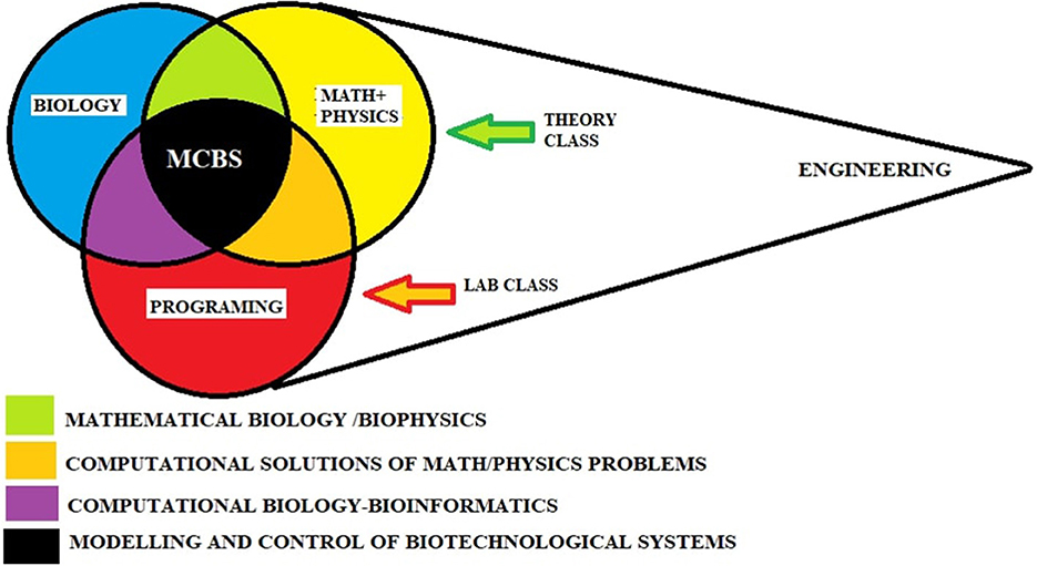
Figure 1. Diverse fields define our PA course. The intersection of all areas is MCBS, modeling and control of biotechnological systems, the core of our proposal.

Before the 2017 and 2019 events, the original agenda items for our PA course were as follows.

2.1 Synthetic program

1. Modeling of dynamical systems.

2. Continuous-Time controllers: PID controllers.

3. Other control strategies.

4. Combinatorial/sequential logic control.

5. Logic control systems (programable logic controllers).

As a consequence of the events that occurred in 2017 and 2019, the latter was modified to more balanced content as follows ³.

2.2 (Modified) synthetic program

1. Space-time evolutionary phenomena in biology: PDE-based models (BM orientation).

2. ODE-based models as a particular case of PDEs (BM, BP orientation).

3. Mass action kinetics (MAK) and basic pathways (BasP), (BM and BP orientation).

4. BP modeling by ODE (BP orientation).

5. Control of BP (BP orientation).

The scheme shown in Figure 2 allowed us to create a new structure for our course, as outlined in Table 1. The subject's content was distributed across 14 themes, which were taught over the 16-week course duration. The grading system consisted of two partial exams and a final project. Approximately, the first partial exam evaluated theme 1. The second exam considered themes 2 and 3, and the final assignment covered the last two issues. More specifically, Table 2 breaks down the content of Table 1, adding the AL technique we considered adequate by theme. The justification of our AL background and organization is described next in part 2.3.

Figure 2

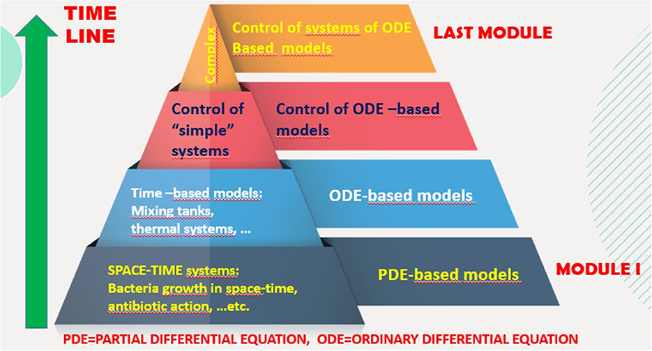
Figure 2. Proposed synthetic program for our PA course. With our proposal, MB students were incorporated into the class, and BP apprentices increased their background in the MB field from a quantitative perspective.

Table 1

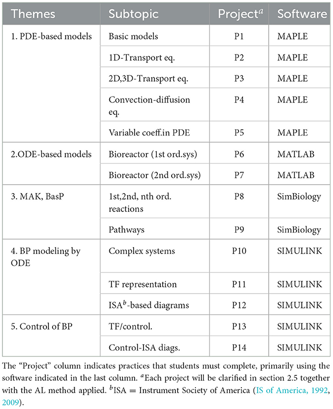
Table 1. Themes, subtopics, and software used in our course during 2020.

Table 2

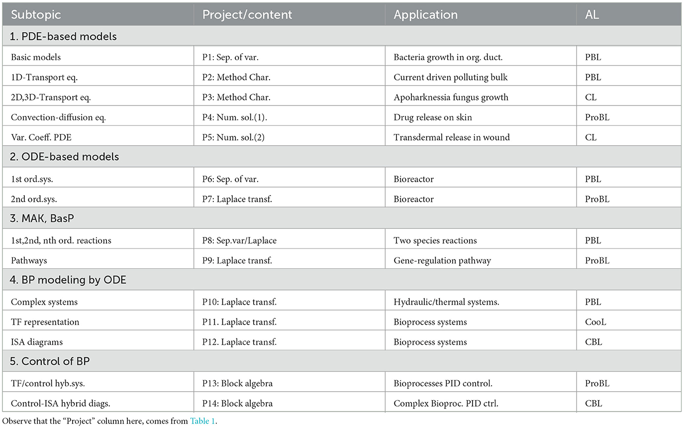
Table 2. Subtopics, projects, content, real application and corresponding AL schemes proposed.

2.3 Planning our PA course according to AL schemes

To ensure our course remains under continuous scrutiny, we adopted the general structure proposed in (Barnes 1989) and (Zavala-Yoe and Ramirez-Mendoza 2019), with our own adaptations. Parts 1 and 2 are sketched in Tables 1, 2, respectively. The remainder is explained in section 3.

1. Organization. Learning goals, outcomes, and general procedures are defined here.

2. Implementation. AL schemes are implemented at this stage.

3. Assessment. Evidence of participants' learning is gathered at this stage.

4. Analysis. Processing of assessment results is currently underway.

5. Improving. Any modifications to the original plan are proposed here.

6. Contrasting. This part was suggested by us to be added as part of our new implementation of enhanced AL to contrast with traditional AL implementations we had in our institute.

7. Outcomes. We also recommend this closing part to summarize the results obtained in the contrasting stage.

We now provide details of the course linked to AL techniques.

2.4 Rationale for our implemented AL strategies

From Part 1, we realized that finding concrete AL techniques combined with generic software for teaching PDEs is rare. Some AL methods were implemented for this theme, but the related software was custom-made, and significant numerical issues arose in those courses. In our case, we aimed to gain a thorough understanding of PDE-based models in biotechnology to grasp the first topic of Table 1. Although our students have a background in multivariate calculus, many of them thought that they would never apply such knowledge in their careers. To circumvent this, we reviewed the basics of partial derivatives to introduce PDEs, utilizing MAPLE assistance and case studies. An additional feature of MAPLE was the development of graphical user interfaces (GUIs) to display the effects of parameter variation on PDEs. After this step, we induced ODEs as a particular case of PDEs (theme 2, Table 1). Furthermore, we motivated this part with real applications, such as bioreactor cases and nth-order reactions (themes 3–4). Finally, from ODEs, we proceeded to the definition of transfer functions and block algebra, which later prompted the need for a controller (themes 4–5).

Thus, the AL procedures implemented in the amended PA course, reported in Table 2, are briefly explained next:

• Problem-based learning (PBL): a problem prompts what the participants should investigate. The problem to be solved arises from a discernible fact. It focuses on gaining new knowledge, while the solution is less relevant (Cornell, 2022).

• Project-based learning (ProBL): the project is divided into tasks that lead to the fabrication of a final invention. What is important is the end product (Boston, 2023).

• Case-based learning (CBL). Knowledge is applied to real-world situations to promote teamwork and examine circumstances (Queen's, 2022).

• Collaborative learning (CL). CL is a teaching technique in which participants work in teams to examine a critical question or create a relevant project (Queen's, 2022).

• Cooperative learning (CooL). CooL is a special type of CL. In CooL, apprentices work together in small groups on certain systematic activities. They are individually responsible for their own work, but the final product of the team is also evaluated (Queen's, 2022; Donnelly and Fitzmaurice, 2005).

Next, we briefly describe the projects indicated in Tables 1, 2 (University of Rochester, 2022; Edwards School of Medicine and Joan, 2022).

2.5 Projects description

As we mentioned at the end of section 1, we specifically developed and improved the final assignment. From our experience, this was a key problem we had to solve.

1. Project 1. PDE-based models. Separation of variables. Bacteria growth in the organic duct. PBL.

Goal: solving a PDE by separation of variables to get a growth model.

2. Project 2. PDE-based models. 1D-Transport equation. Method of characteristics. The bulk of the pollutant driven by a stream. PBL.

Goal: solve a first-order PDE by the method of characteristics to model the motion of pollutants. An example of this solution is given in Equation 1 where u(x, t) is the pollutant trajectory.

$\begin{array}{r}\frac{\partial u}{\partial t}-D\frac{\partial u}{\partial x}=Q(x,t),\\ u(x,0)=0,u(0,t)=0\\ \Rightarrow u(x,t)=f(x+Dt),D\in \Re & (1)\end{array}$

3. Project 3. PDE-based models. 2D,3D-Transport equation. Method of characteristics. Apoharknessia fungi growth (Garrett, 2019). CL.

Goal: applying a PDE to represent fungi evolution in 2D and 3D. This expansion u(x, t) (or u(x, y, t) in Equation 2) is modified by nutrients Q. For Q(x, y, t) = 0, the solution can be analytically obtained. If Q(x, y, t)≠0, a numerical method is needed ⁴.

$\begin{array}{r}\frac{\partial u}{\partial t}-D\left(\frac{\partial u}{\partial x}+\frac{\partial u}{\partial y}\right)=Q(x,y,t),u(x,y,0)=f(x,y),\\ \Rightarrow u(x,y,t)=f(x+Dt,y+Dt),D\in \Re & (2)\end{array}$

4. Project 4. PDE-based models. Convection-diffusion equation. Numerical solutions. Drug release through skin (Kathe and Kathpalia, 2017). ProBL. A real case of autoimmune leukocytoclastic vasculitis wounds (Órfão et al., 2023; Sunderktter et al., 2023) was presented and followed here to apply the content of themes 4–5. Observe Figure 3 where a healing process is modeled via PDEs.

Figure 3

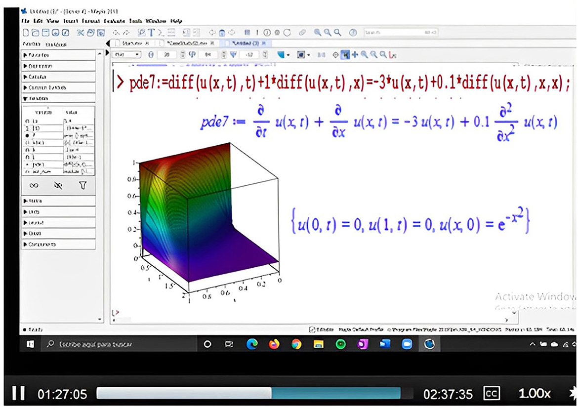
Figure 3. Zoom session during which an advection-diffusion PDE was numerically solved, producing a solution surface for a transdermal phenomenon. The material penetrates the skin according to u(x, t) along the x-axis. Matter is initially distributed along “x” (red), but as it infiltrates, its amount decreases (blue). At the same time, this matter decreases as t increases.

Goal: modeling 1D convection-diffusion into skin. A generic case of this model⁵ is given by Equation 3.

$\begin{array}{r}\frac{\partial u}{\partial t}+a\frac{\partial u}{\partial x}+b\frac{\partial u^2}{\partial x^2}+cu=Q(x,t),\\ u(x,0)=f(x),u(0,t)=g_1(t),u(1,t)=g_2(t).& (3)\end{array}$

The MAPLE code for numerically solving Equation 3 is given below as an example. The terms of the equation were rearranged to align with the screen shown in Figure 3, where the outcome is displayed. There, a = 1,b = −0.1,c = 3, f(x, 0) = e^−x2, Q(x, t) = 0 and Q(x, t)≠0. The amount of substance tends to decrease in t and x at a slow pace, particularly for low values of t.

pde:=diff(u(x,t),t) + (diff(u(x,t),x)=0.1*diff(u(x,t),t,t)-3*u(x,t)=Q;

ic:={u(x,0)=exp(-x ∧2),u(1,t)=0,u(0,t)=0}

sol:=pdsolve(pde,ic,numeric,time=t,range=0..1).

5. Project 5. PDE-based models. Space variable convection-diffusion PDE. CL.

Goal: modeling of a transdermal (Kalia and Guy, 2001) medical substance applied in a wound. The challenge for the students here is that the coefficients in the convection-diffusion PDE (Equation 3 above) are variable in 2D-space and time. The structure of the PDE shown in Figure 3 is the same as in project 4, but the coefficients are much more complex, thereby more faithfully reproducing the reality of the anomaly⁶.

6. Projects 6 and 7. ODE-based models. Bioreactor sections. PBL, ProBL, respectively. Since these situations are similar, we will describe them together here.

Goal: identifying equivalence between differential equations and transfer functions with SIMULINK support. Special attention to bioreactor models.

7. Projects 8 and 9. Biological cases. ODE as models. PBL, ProBL, resp.

Goal: modeling of BasP and MAK using SimBiology (Mathworks, 2022b). Students realized that ODEs are not only useful for representing physical devices (bioreactors) but also biological phenomena.

8. Projects 10–12. Transfer functions. Complex open-loop systems. PBL, CooL, and CBL, respectively.

Goal: representing higher-order structures using block diagrams. An example of this is the 6th-order hydraulic installation shown in Figure 4.

Figure 4

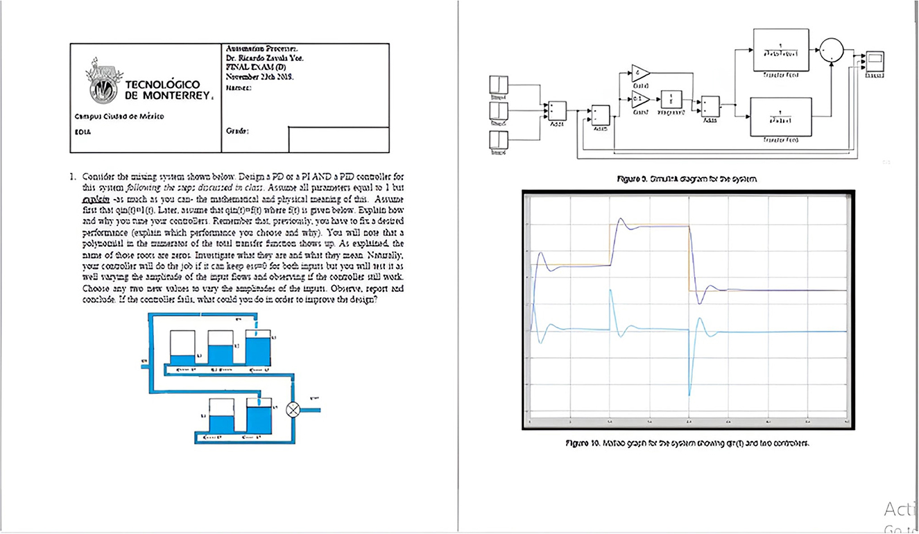
Figure 4. First two pages of the student report. It is worth noting how they interpreted a complex system to create a block diagram suitable for SIMULINK simulations.

9. Projects 13, 14. ProBL, CBL, resp. Controlled bioprocesses. Block diagrams. ISA standards.

Goal: representing complex hybrid⁷ systems according to ISA rules. Design of controllers. See Figure 5.

Figure 5

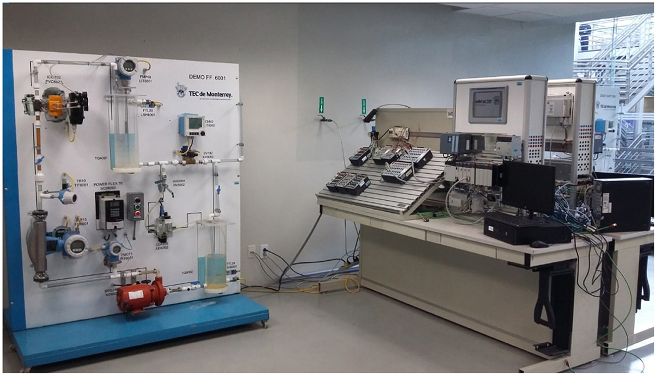
Figure 5. One of our automation stations at our institute, where our students learn modeling and control of hydraulic and hybrid systems in biotechnology. Besides, a PLC controller is also programmed for this purpose.

3 Results

Previous sections have aimed to demonstrate the step-by-step development of our proposed AL system. We have remarked that the use of specialized software was key. Common activities and assignments were constrained by the available software and learning strategies throughout this period. Table 3 shows the specialized software used from 2015 to 2020 and the most representative learning actions associated with them. There, “Rep” indicates if special reports were requested about certain activity considered important. “Expo” means that students presented a topic by themselves at least once a semester. “SMLK” denotes SIMULINK, and “V” if at least one video was considered. We observed that the acquisition and updating of software was significant in 2020. This was confirmed by the students' grades (Table 4) and their evaluations of the teachers (illustrations 6 and 7)⁸.

Table 3

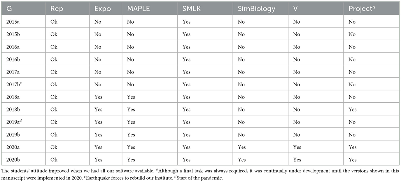
Table 3. Specialized software used in our course from 2015 to 2020 and complementary activities: “V” means video presentation, and “Project” indicates an additional task.

Table 4

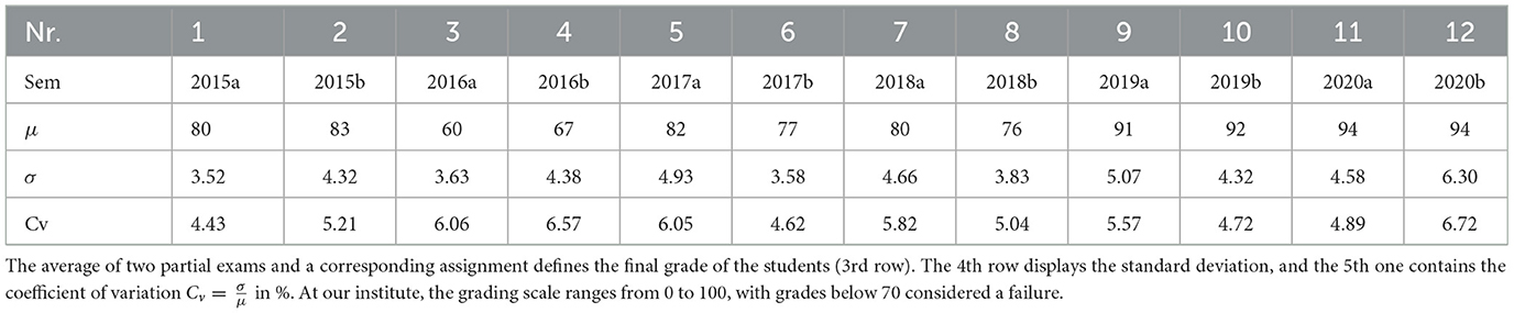
Table 4. Grades of students from semester 1 to 12 (2015–2020).

Figure 6 shows a sample of an official students survey (2018b) where a positive mention of metodologia computacional, (computational methodology) is highlighted⁹. Figure 7 reflects satisfaction with course planning.

Figure 6

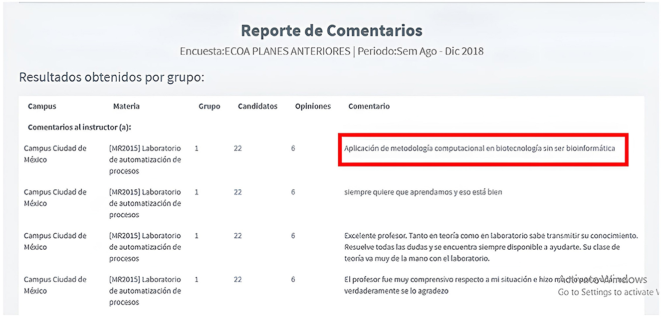
Figure 6. Students survey, taken from official institute site (2018b). Twenty-two persons enrolled, 6 (positive) opinions; one of them about computational tools (inside the red box it can be read “Aplicación de Metodologia Computacional,” i.e., “(Performance of) Application of Computational Methodology.” Below it: “He (the teacher) always wants the students to learn.” Third row: “Excellent teacher....” Fourth row: “The teacher was very understanding with respect to my situation, I'm really thankful to him.”

Figure 7

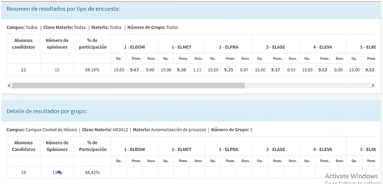
Figure 7. At the end of each term, students typically complete a survey. As an example, we present an excerpt from 2018b (top panel, 22 students with 15 opinions) and 2018a (bottom panel, 19 students with 13 opinions), respectively. There they show their degree of satisfaction (base 10) whose average is given in bold. The main measures are: ELMET = Methods and technology, ELPRA = Practical application, ELASE = Mentoring, - ELEVA = Evaluation, and ELRET=Intellectual challenge.

Based on all this information, we felt confident about our achievements. However, to be more objective, we present the following statistical study, which provides a deeper insight.

3.1 Statistical analysis

An investigation of student achievement from 2015 to 2020 was not planned. As we explained, we suddenly found ourselves in a problematic situation, one that the students of Process Automation faced during the reconstruction of our institute and the pandemic. Besides, the alumni had a fundamental disadvantage in mathematics and programming. Therefore, after years of experience, we decided to collect information to evaluate the results of our modifications. In this spirit, as a preliminary stage, an analysis of our students' performance was practiced via the semester averages of the three grades (two exams and a final activity). These parameters gave us an early feeling of confidence about the improvements we designed. The total averages are shown in Table 4. The first and second semesters of a year are denoted by (a) and (b), respectively. The student's grading scale is based on 100, i.e., the lowest score is 0/100 and the highest is 100/100.

As can be seen, 2015 appears to reflect some improvisation and rapid adaptation to the initial changes. The latter implies a certain level of tolerance and understanding of our participants, with averages of 80 and 83 (columns 1 and 2, respectively). After that, we noticed in our classrooms a clear adaptation reaction that occurred during 2016 with a drastic decrease to 60 and 67. Subsequently, the experience gained over this period allowed us to have a more stable environment in 2017a, achieving an 82. Despite the improvement, the 2017b earthquake forced us to wait weeks to create an innovative work environment. Thus, a remote learning tactic had to be executed quickly. These events influenced the group average, resulting in a 5-point reduction to achieve 77. 2018 shows a readjustment, with the number rising from 77 to 80 but then falling again to 76. However, what happened in 2019 is quite interesting because, in the face of the emerging pandemic, we were able to work remotely and utilize virtual learning environments. 2019 was a year in which the averages improved significantly. This positive trend continued from 2019 to 2020. In that year, we observed a consistent trend with improved achievements of 94 in both semesters.

The latter perceptions align with the coefficient of variation, which exhibits a clear upward trend from 2015 to 2017 (Table 4). A sudden drop occurs in 2017b (earthquake), followed by a recovery period with almost no variation from 2018a to 2019a. Subsequently, there is another drop in 2019b (pandemic). In 2020, an upward trend occurred again.

A more in-depth interpretation was produced using the student's grade record instead of the simple averages. As mentioned, each record is composed of two partial exams and a final assignment. Therefore, we considered that the comparison between the average of the two exams X vs. the final assignment F was key. Since the period under investigation is 2015–2020, there were 12 groups to work with. We wish to determine if there was a significant change in the 12 groups, considering both the midterm grade and our final activities for each participant. Thus, for each group, we computed the difference δ = F−X for each student. The number of pupils in our groups always changes; however, our institution considers a number of students between (15, 35) per class. To determine whether a parametric or non-parametric test should be applied, the normality of the data was assessed. For this, a Shapiro-Wilk test revealed that our data did not behave normally at a 5% significance level. In addition, the n_i, i = 1..12 of our groups are small (n_i < 50) (Dekking et al., 2005; Martinez-Gonzalez, 2020). Consequently, a non-parametric test was carried out in 2 stages¹⁰: an internal one (comparing partial grades vs. final work per class) and an external one (contrasting groups) in this way:

3.2 Steps

1. δ_ij was calculated for each group i = 1, ..., 12, and for each participant j. From this, a Wilcoxon signed test (WST) was applied to determine whether the population median is significantly different from zero.

2. This second step involves practicing a two-sample Wilcoxon rank sum test (WRST) to compare results at relevant moments. Thus, we decided to contrast the first group we dealt with (2015a) vs. the group (2017b, earthquake); later (2015a) vs. (2020b, end). Additionally, (2017b) vs. (2020b), as 2020b was the semester during which our active learning procedures were already in place. Therefore, we have to oppose δ₁ vs. δ₆, δ₆ vs. δ₁₂ and δ₁ vs. δ₁₂ to determine whether the improvements were significantly distinct.

3.3 Outcomes

1. Before applying a WRT, we first obtained non-parametric univariate statistics for each (group) deviation δ_i. A summary of the distribution of scores (center and spread) is presented in Table 5. A quick look at the medians shows that (excluding groups of semesters 3 and 4) there was an improvement from the partial exams average to the final assignment. Thus, 50% of the students showed improved learning in 10 out of 12 groups. Nonetheless, apprentices in groups 3 and 4 performed worse, as evidenced by the appearance of negative values. Indeed, there is a contrast between the years 2015 and 2016, as well as between 2016 and 2017. The explanation may be that we started implementing our strategy gradually in 2015, but it became more established in 2016. Thus, we believe that the reaction to new activities (particularly the final project) is reflected with more effort during partial exams than in the course of the final task. Paying attention now to 2017, we observe that the numbers evolve to positive, although 2017b descends by almost 50% with respect to 2017a. The explanation could be that at this time, the consequences of the terrible event manifested in this way. The up-and-down effect in the medians of δ repeats in 2018 with 11.35 and 3.41 in what appears to be a stabilization season. However, we suddenly face the minimum value in 2019a (1.45), the moment at which the pandemic emerged. The transition from 2019b to 2020a occurs with little change according to the numbers, but with a clear upward trend in 2020b. Paying attention to the inter-quartile row I_qr, it can be noticed that the year with more variability is 2019. In contrast, periods 2 (2015b with I_qr = 3.93) and 6 (2017b, I_qr = 3.37) are those with the least dissimilarity between the midterm average and the final project. These seasons appear to be times of tolerance in students performance.

On the other hand, Table 6 reflects the results of a WST run for each δ_i. This procedure tests the null hypothesis of equal medians at the default 5% in two vectors against the alternative of not equal medians ¹¹. From this part, we can see that improvements in classes were significantly different from zero in 9 out of 12 groups. Indeed, excluding semesters 9–11, i.e., 2019a, 2019b, and 2020a, the other periods display ρ < 0.05 and a logical value of h = 1 (true). This means taking the alternative hypothesis of true location not equal to zero or the rejection of the null hypothesis of equal medians at the default 5% significance level. For semesters 9–11, we do not reject the hypothesis of equal medians.

2. Before applying a WRST, we wanted to determine whether the measures of improvements in all groups were significantly distinct by box plot graphs. In Figure 8, the box plot of each δ_i is presented. As is known, notches typically do not overlap if median values are significantly different from each other at the 5% level. Besides, we can observe that the box plots are not symmetrically drawn. This occurs when data probability distributions are not normally distributed. Additionally, it is notable that the position of the first four box plots stands out. The first year, the medians of δ were large positive, but large negative the following year. Another notable feature is the presence of outliers during the first year of our registry; this may be the result of the initial phase of our adaptations. After 2 years (starting from the fifth semester), the medians of δ are almost within the band of [0, 10] points, indicative of a more stable period. However, the box plot corresponding to the 5th semester (2017b, earthquake) exhibits unusual behavior due to its “flipped” appearance. The explanation about why notches extend beyond the 25th and/or 75th percentiles is due to the uncertainty of the true median value. This occurs if a sample size is relatively small [recall that there is a denominator $\sqrt{n}$ to compute the notch height (Dekking et al., 2005)]. Particularly in 2017a, there was a decrease in the number of students enrolled in all courses. Also noteworthy is the case of 2019b (10th semester), when our institute suspended classes and in-person activities due to the COVID pandemic. Finally, despite fluctuations, the medians of δ over the last 2 years tend to be more stable (and with an improvement in grades, see Table 4).

We now move on to an examination of δ between critical seasons that can confirm the results and observations obtained so far. Although there are many combinations we could investigate, we aimed to determine whether the amount of improvement across key periods differed significantly. For this purpose, we chose to compare semester 1 (2015a) with semester 6 (2017b, earthquake); semester 6 with semester 12 (2020b, improved AL); and semester 1 with semester 12 (extremes). From the same figure (or from Table 5), the medians of groups 1, 6, and 12 are 19.54, 3.89, and ≈6, respectively. These numbers denote that there was an (unequal) improvement in these times of F with respect to X. By 2020b, having achieved a 6-point improvement during a stable season with an average final grade of 94 (Table 4), this was truly remarkable.

Table 5

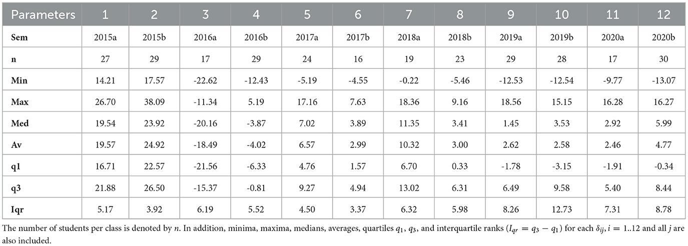
Table 5. Descriptive statistics for δ.

Table 6

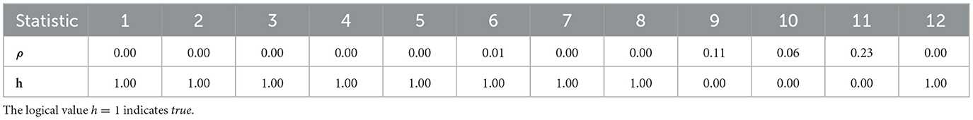
Table 6. Information produced in MATLAB regarding the Wilkinson signed test to assess if improvements by group were significantly greater than zero.

Thus, if we observe this unusual “flipped” appearance in the notched box plots, it simply means that the first quartile has a lower value than the confidence interval of the mean, and vice versa for the third quartile. Although it may look unappealing, it provides useful information about the (un)confidence of the median.

Next, a formal WRST tests the null hypothesis that the data in two vectors are samples with equal medians against the alternative that they are not, with significance at the 5% level. The outcomes of this part are shown in Table 7. Significant differences from zero are observed in groups 1 vs. 6 and 1 vs. 12. This indicates that a real improvement has occurred since the detection of the problem (2015a) in comparison to 2017b (earthquake) and from then to 2020b (the advanced stage of our plan). This was not the case during the middle period (from the 6th to the 12th class).

Table 7

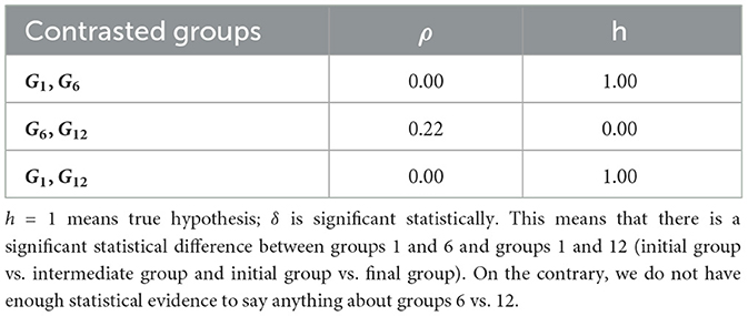
Table 7. Wilcoxon rank sum test to contrast groups 1,6,12.

Calculation of effect size (side effect). As in any statistical test, not only the ρ value must be indicated, but also the size of the observed effect, since this will allow us to determine whether, in addition to being significant, the difference is practical. The effect size for a Mann-Whitney-Wilcoxon test or Wilcoxon rank-sum test is usually calculated from the z-factor with $r_{RCC}=z/\sqrt{n}$ where n is the total number of samples of all records p, i.e., n = n₁+⋯+n_p (Pallant, 2016). The value of z is produced by MATLAB when the Wilcoxon tests are run. From the latter, a set of values for r_RCC was obtained: r_{RCC1, 6} = 0.23, r_{RCC6, 12} = −0.03, r_{RCC1, 12} = 0.21. These values are classified according to the following scale of correlation (Bartz, 1999; Rosenthal, 1994):

• 0 < r_RCC < 0.2: very low.

• 0.2 ≤ r_RCC < 0.4: low.

• 0.4 ≤ r_RCC < 0.6: moderate.

• 0.6 ≤ r_RCC < 0.8: strong.

• 0.8 ≤ r_RCC < 1: very strong.

Their statistics are given at the end of Table 8. It can be deduced that there is a stronger relation between groups (1,6) and (1,12) than between (6,12). Despite its simplicity, r_RCC has some drawbacks. This parameter is sensitive ¹² to the size of n, i.e., to each n_i, i = 1, ..., p. Consequently, the rank biserial coefficient ¹³ (RBC) is preferred to report effect size estimates in Wilcoxon tests (Dekking et al., 2005; Martinez-Gonzalez, 2020; Rosenthal, 1994; Pallant, 2016). Consequently, r_RBC is defined as (Tomczak and Tomczak 2014):

$\begin{array}{ll}{r}_{RBC}=\frac{4\left[T-\left(\frac{R_1+R_2}{2}\right)\right]}{n(n+1)}& (4)\end{array}$

Above, T = min(R₁, R₂), where R₁ is the sum of ranks with positive signs, and R₂ is the sum of ranks with negative signs. n is the total sample size. The scale of r_RBC is shown below (Cohen, 1988).

• r_RBC < 0.1: very small.

• 0.1 ≤ r_RBC < 0.3: small.

• 0.3 ≤ r_RBC < 0.5: moderate.

• r_RBC>0.5: large,

Table 8

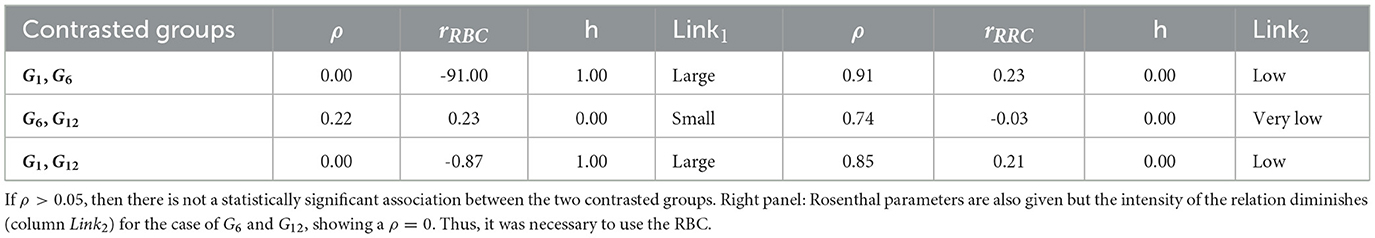
Table 8. Rank biserial coefficients for the compared cases.

In Table 8, these parameters were determined to compare groups G₁ vs. G₆, G₆ vs. G₁₂, and G₁ vs. G₁₂ (Kerby, 2014). Negative signs indicate inverse variation. In these cases, if the difference between groups increases, the other one decreases.

The RBC parameters (left side of Table 8) allow us to conclude about the significance of the differences in medians. Since group 1 has a median of 19.54 and group 6 of 3.89, δ_{1, 6} = 19.54 − 3.89 = 15.65 ¹⁴. We can decisively conclude that we reject the null hypothesis of equal medians at 5% of significance in groups 1 vs. 6, where a difference of 15.65 points represents a small improvement of class 1 with respect to class 6. The same happens with classes 1 and 12 for δ_{1, 12} = 19.54 − 5.99 = 13.55. However, since δ_{6, 12} = 5.99 − 3.89 = 2.10, we cannot reject the hypothesis of equal medians where a difference of 2.10 represents a very low improvement of group 6 vs. class 12. In addition, the signs indicate inverse variations. Increasing the medians in one group would mean decreasing those in the other. The reason for this could be the advancement of the strategy in period 12 with respect to period 6. There could also have been a more tolerant environment during the time of class 6, which would contrast with a less tolerant environment during class 12, hence explaining the reverse effect in this combination. Additionally, from Figure 8, groups 1 and 6 present small variations with respect to class 12, but class 6 has an outlier (2017).

Figure 8

Figure 8. Boxplots for δ corresponding to all groups. Notice the extreme behavior in the medians of δ during the first 2 years (semesters 1–4), as well as the presence of outliers. From the 5th semester onwards, the trend was relatively stable, although notable developments occurred in semesters 6 (2017b, earthquake), 10 (2019b, pandemic), and 12 (2020b, steady state of our AL implementation). Additionally, longer whiskers suggest that the data points in that tail are more dispersed and potentially less clustered around the central tendency.

4 Discussion

As established from the beginning, the original program of the course had to be modified because of difficulties, reluctance, and the background of the students. Once we implemented the altered synthetic program, we noticed a decisive improvement. However, we found that students had not fully grasped the mathematical concepts and were unable to apply them to complex contexts in biotechnology. That is why we had to supervise them closely, providing special activities and software support. The latter, combined with advancing AL methods, was a boon to refine the overall level of our groups. Although the catastrophes we faced in 2017b and 2019a affected our city and the whole world very seriously, they forced us to develop remote learning with all its implications. Although we observed a qualitative success of our plans, we later confirmed that via descriptive statistics as a first numerical approach. All this was clearly confirmed by a serious statistical study. All these strategies contributed to our study performance, despite not having been previously planned.‘

5 Limitations

It is worth mentioning that potential biases, such as the Hawthorne effect, should be briefly addressed here due to changes in methodology. This phenomenon is a type of behavioral reactivity in which individuals modify an aspect of their behavior upon becoming aware that they are being observed (McCarney R, 2007). However, since our study was not planned and the students were not aware that they were being monitored to evaluate AL activities, we believe that this effect did not substantially affect the results. On the other hand, some minor adjustments may be necessary to accommodate specific situations. Our methodology remains stable and is consistent with our design.

6 Conclusion

From the early stages of teaching the PA course, we detected inconveniences that had not been corrected. Subsequently, the course program was adapted to be more useful for concentrations of MB and BP students, rather than just one. During the implementation of our new methodology, we observed gradual changes in students' attitudes and abilities. Moreover, with the help of specialized software, as well as convenient monitoring and the development of a remote learning mode, we definitively refined the performance of our students. To adopt this approach, after applying the active learning techniques described here, researchers and educators can statistically substantiate their results using the tests employed. While this innovation can be applied to other STEM courses, we believe minimal adaptations are required.

Data availability statement

The raw data supporting the conclusions of this article will be made available by the authors, without undue reservation.

Ethics statement

Ethical approval was not required for the studies involving humans because our study used only numerical data without paying attention to personal information. The studies were conducted in accordance with the local legislation and institutional requirements. Written informed consent for participation was not required from the participants or the participants' legal guardians/next of kin in accordance with the national legislation and institutional requirements.

Author contributions

RZ-Y: Conceptualization, Data curation, Formal analysis, Funding acquisition, Investigation, Methodology, Project administration, Resources, Software, Supervision, Validation, Visualization, Writing – original draft, Writing – review & editing.

Funding

The author(s) declare that no financial support was received for the research and/or publication of this article.

Acknowledgments

I would like to thank Carolynn Hill (MAPLESOFT) for her kind permission to use the MAPLE software-free of charge-for our students for over a year.

Conflict of interest

The author declares that the research was conducted in the absence of any commercial or financial relationships that could be construed as a potential conflict of interest.

Generative AI statement

The author(s) declare that no Gen AI was used in the creation of this manuscript.

Publisher's note

All claims expressed in this article are solely those of the authors and do not necessarily represent those of their affiliated organizations, or those of the publisher, the editors and the reviewers. Any product that may be evaluated in this article, or claim that may be made by its manufacturer, is not guaranteed or endorsed by the publisher.

Footnotes

1. ^Remark: The use of software (MAPLE, MATLAB) does not imply commercial sponsorship or bias. They were used for their known scientific-technical-computational advantages.

2. ^Compare our new/additional skills vs. the old ones here: https://samp.itesm.mx/Materias/VistaPreliminarMateria?clave=MR2012&lang=EN.

3. ^The main phase of this development took place in 2020.

4. ^Actually, a real fungal growth experiment was conducted here in a Petri dish. The evolution of real fungi was contrasted with PDE-based models, with enthusiastic reactions from students. This activity was developed from Project 1–Project 3.

5. ^In this instance, as well as in systems 2, 3, the coefficients could be functions of x,y,t, and a numerical value had to be used. This fact was very attractive to students.

6. ^This means that they have to propose model ?? with a = a(x, y, t), b = b(x, y, t), c = c(x, y, t).

7. ^Hybrid means here a combination of several types of structures (hydraulic, thermal, and mechanical systems).

8. ^Ethics committee approval was not required, as the survey was completed anonymously. See also part Informed consent.

9. ^There were more positive comments about the use of all this software, but we could show one as an example.

10. ^The tests of this section were run in MATLAB.

11. ^Data were adjusted via Holm-Bonferroni correction.

12. ^This parameter is sometimes referred to as Rosenthal's correlation coefficient, RCC (Rosenthal, 1994).

13. ^The number of methods that report effect size measures for the Mann-Whitney U test, Wilcoxon tests are rather scanty (Fritz et al., 2012; Tomczak and Tomczak, 2014; Glass, 1965).

14. ^Here we use symbols G and δ indistinctly.

References

Alam, M. N. H. Z., and Zakaria, Z. Y. (2021). Application of computational tools to support cooperative learning in bioreactor design course. Int. J. Emerg. Technol. Learn. 16, 46–61. doi: 10.3991/ijet.v16i15.23697

Crossref Full Text | Google Scholar

Alfonseca, M., de Lara, J., and Montoro, G. (2002). “Teaching partial differential equations trough internet: an interactive approach,” in 16th European Simulation Multiconference (ESM'2002) (Darmstadt), 395–399.

Google Scholar

Ballesteros-Martin, M. M., and Moral-Rama, A. (2014). Using simulation software to implement an active learning methodology in the university teaching. Int. J. Educ. Res. Innov. 1. Available online at: https://www.upo.es/revistas/index.php/IJERI/article/view/884

Google Scholar

Barnes, D. (1989). Active Learning. Leeds University, UK, TVEI Support Project. 1 Edition.

Google Scholar

Bartz, A. E. (1999). Basic Statistical Concepts. Upper Saddle River, New Jersey, 4 edition.

Google Scholar

Boston, U. (2023). Project-based learning: teaching guide. Available online at: https://www.bu.edu/ctl/guides/project-based-learning/ (Accessed February 9, 2023).

Google Scholar

Cano, M. J., Chacpn-Vera, E., and Esquembre, F. (2015). Bringing partial differential equations to life for students. Eur. J. Phys. 36:35026. doi: 10.1088/0143-0807/36/3/035026

Crossref Full Text | Google Scholar

Cohen, J. (1988). Statistical Power Analysis for the Behavioral Sciences. Routledge, New York, 2nd edition.

Google Scholar

Cornell, U. (2022). Center of teaching innovation, center of teaching innovation web site. Available online at: https://teaching.cornell.edu/teaching-resources/engaging-students/problem-based-learning (Accessed February 9, 2023).

Google Scholar

de Monterrey, T. (2019). Al and remote mode during pandemic 2019. Available online at: https://observatorio.tec.mx/edu-bits-blog/la-regeneracion-de-los-habitos-de-estudio-en-universitarios-durante-la-pandemia/ (Accessed December 26, 2023).

Google Scholar

Dekking, F. M., Kraaikamp, C., Lopuha, H. P., Meester, L. E., and Modern, A. (2005). Introduction to Probability and Statistics. Springer: New York. doi: 10.1007/1-84628-168-7

Crossref Full Text | Google Scholar

Donnelly, R., and Fitzmaurice, M. (2005). “Collaborative ProBL and PBL in higher educ.: a consideration of tutor and student role in learner-focused strategies,” in Emerging Issues in the Practice of University Learning and Teaching, eds. G. O'Neill, S. Moore and B. McMullin (All Ireland Society for Higher Education (AISHE): Dublin).

Google Scholar

Edwards School of Medicine M. U. Joan C. (2022). Learning-objective-writing. Available online at: https://jcesom.marshall.edu/media/54756/learning-objective-writing.pdf (Accessed March 7, 2023).

Google Scholar

Felse, P. A. (2018). Pedagogical approaches to teach fluid mechanics and mass transfer to nonengineers with biotechnology focus. Chem. Eng. Educ. 52. Available online at: https://www.scholars.northwestern.edu/en/publications/pedagogical-approaches-to-teach-fluid-mechanics-and-mass-transfer

Google Scholar

Fritz, C. O., Morris, P. E., and Richler, J. J. (2012). Effect size estimates: current use, calculations, and interpretation. J. Exp. Psychol. Gen. 141, 2–18. doi: 10.1037/a0024338

PubMed Abstract | Crossref Full Text | Google Scholar

Garrett, A. (2019). Mycelial growth and sporulation of apoharknessia eucalyptorum on different culture media. Summa Phytopathol. 45, 272–278. doi: 10.1590/0100-5405/207327

Crossref Full Text | Google Scholar

Glass, G. V. (1965). A ranking variable analogue of biserial correlation: implications for short-cut item analysis. J. Educ. Meas. 2, 91–95. doi: 10.1111/j.1745-3984.1965.tb00396.x

Crossref Full Text | Google Scholar

Hough, M., Wood, E., Yip, W. S., and Marlin, T. (2002). “A web site to support active student learning in process control,” in Proceedings of the 2002 American Society for Engineering Education Annual Conference and Exposition (American Society for Engineering Education).

Google Scholar

IS of America. (1992). ANSI/ISA-S5.1-1984 (R 1992). Instrumentation Symbols and Identification, North Carolina, USA, 2 edition.

Google Scholar

IS of America. (2009). ANSI/ISA-5.1-2009. Instrumentation Symbols and Identification, North Carolina, USA, 2 edition.

Google Scholar

Kalia, Y. N., and Guy, R. H. (2001). Modeling transdermal drug release. Adv. Drug Deliv. Rev. 48, 159–172. doi: 10.1016/S0169-409X(01)00113-2

PubMed Abstract | Crossref Full Text | Google Scholar

Kathe, K., and Kathpalia, H. (2017). Film forming systems for topical and transdermal drug delivery. Asian J. Pharm. Sci. 12, 487–497. doi: 10.1016/j.ajps.2017.07.004

PubMed Abstract | Crossref Full Text | Google Scholar

Keener, J. P., and Sneyd, J. (2009). Mathematical Physiology. Interdisciplinary Applied Mathematics, Springer: New York. doi: 10.1007/978-0-387-75847-3

Crossref Full Text | Google Scholar

Kerby, D. S. (2014). The simple difference formula: an approach to teaching nonparametric correlation. Innov. Teach. 1. doi: 10.2466/11.IT.3.1

PubMed Abstract | Crossref Full Text | Google Scholar

Lozada, E., Guerrero-Ortiz, C., Coronel, A., and Medina, R. (2021). Classroom methodologies for teaching and learning ordinary differential equations: a systemic literature review and bibliometric analysis. Mathematics 9:745. doi: 10.3390/math9070745

Crossref Full Text | Google Scholar

Martinez-Gonzalez, M. A. (2020). Bioestadistica Amigable. Elsevier.

Google Scholar

Mathworks, T. (2022a). Matlab. Available online at: https://la.mathworks.com/discovery/what-is-matlab.html (Accessed February 26, 2023).

Google Scholar

Mathworks, T. (2022b). Simbiology. Available online at: https://la.mathworks.com/help/simbio/ (Accessed February 26, 2023).

Google Scholar

Mathworks, T. (2022c). Simulink. Available online at: https://la.mathworks.com/products/simulink.html (Accessed February 2, 2023).

Google Scholar

McCarney, R., Warner, J., Iliffe, S., van Haselen, R., Griffin, M., and Fisher, P. (2007). The hawthorne effect: a randomised, controlled trial. BMC Med. Res. Methodol. 7:30. doi: 10.1186/1471-2288-7-30

PubMed Abstract | Crossref Full Text | Google Scholar

Myers, J., Trubatch, D., and Winkel, B. (2008). Teaching modeling with partial differential equations: several successful approaches. PRIMUS 18, 162–182. doi: 10.1080/10511970701643889

PubMed Abstract | Crossref Full Text | Google Scholar

Órfão, A., Madeira, D., Duarte, D. M., Pereira, F. G., and Matos, C. (2023). Gabapentin-induced cutaneous leukocytoclastic vasculitis: a case report. Cureus 15:e44616. doi: 10.7759/cureus.44616

PubMed Abstract | Crossref Full Text | Google Scholar

Pallant, J. (2016). SPSS Survival Manual. McGraw-Hill-Education, 6th edition. London, UK.

Google Scholar

Queen's, U. (2022). Center for teach. and learn., Canada, case based learing. Available online at: https://www.queensu.ca/ (Accessed February 8, 2023).

Google Scholar

Rodriguez, M., Diaz, I., Gonzalez, E. J., and Gonzalez-Miquel, M. (2018). Motivational active learning: an integrated approach to teaching and learning process control. Educ. Chem. Eng. 24, 7–12. doi: 10.1016/j.ece.2018.06.003

PubMed Abstract | Crossref Full Text | Google Scholar

Rosenthal, R. (1994). “Parametric measures of effect size,” in The Handbook of Research Synthesis, eds. H. Cooper and L. V. Hedges (Russell Sage Foundation: New York).

Google Scholar

Soft, M. (2022). Maple. Available online at: https://cn.maplesoft.com/index.aspx (Accesed February 2, 2023).

Google Scholar

Sunderktter, C., Golle, L., Pillebout, E., and Michl, C. (2023). Pathophysiology and clinical manifestations of immune complex vasculitides. Front. Med. 10:1103065. doi: 10.3389/fmed.2023.1103065

PubMed Abstract | Crossref Full Text | Google Scholar

Tomczak, M., and Tomczak, E. (2014). The need to report effect size estimates revisited: an overview of some recommended measures of effect size. Trends Sport Sci. 1.

PubMed Abstract | Google Scholar

University of Rochester M. C.. (2022). Writing-clear-learning-objectives. Available online at: https://www.urmc.rochester.edu/MediaLibraries/URMCMedia/center-experiential-learning/about-us/images/Writing-Clear-Learning-Objectives.pdf (Accessed January 29, 2023).

Google Scholar

Zavala-Yoe, R. (2008). “Modelling and control of dynamical systems: numerical implementation in a behavioral framework, volume 124,” in Studies in Computational Intelligence (SCI) (Springer: New York).

Google Scholar

Zavala-Yoe, R., Iqbal, H. M. N., and Ramirez-Mendoza, R. A. (2019). Understanding the evolution of pollutants via hierarchical complexity of space-time deterministic and stochastic dynamical systems. Sci. Total Environ. 710:136245. doi: 10.1016/j.scitotenv.2019.136245

PubMed Abstract | Crossref Full Text | Google Scholar

Zavala-Yoe, R., and Ramirez-Mendoza, R. (2019). EEG acquisition and analysis to improve stochastic processes and signal processing understanding in engineering students: refining active learning dynamics via interactive approach in teaching. Int. Jour. on Int. Des. and Manuf . 13. doi: 10.1007/s12008-019-00601-7

Crossref Full Text | Google Scholar