Multi-Fluid Computational Fluid Dynamic Predictions of Turbulent Bubbly Flows Using an Elliptic-Blending Reynolds Stress Turbulence Closure

The accurate prediction of bubbly flows is critical to many areas of nuclear reactor thermal hydraulics, mainly, but not only, in relation to the key role bubble behavior plays in boiling flows. Large scale computations of flows with hundreds of thousands of bubbles are possible at a reasonable computational cost using computational fluid dynamic, multi-fluid Eulerian-Eulerian models. The main limitation of these models is the need to entirely model interfacial transfer processes with proper closure relations. Here, the capabilities and advantages provided by a model that includes an elliptic-blending Reynolds stress turbulence closure (EB-RSM), allowing fine resolution of the velocity field in the near-wall region, are tested over a large database. This database includes mostly monodispersed bubbly flows over a wide range of operating conditions and geometrical parameters, including upward and downward pipe flows, large diameter pipes and a square duct. The model shows encouraging accuracy and robustness, with good agreement over most void fraction distributions and accurate prediction of the magnitude and position of the near-wall void fraction peak. The model does not include any wall force, avoiding all the related uncertainties, and the prediction of the void fraction peak relies on the fine resolution of the near-wall pressure gradient induced by the turbulence field. Overall, the EB-RSM allows accurate resolution of the velocity and turbulence field near the wall, and the transition to this and similar turbulence closures is of value in assisting the ongoing quest for thermal hydraulic models that are accurate and of general applicability. Additional modifications to the near-wall modeling approach, which is still based on its single-phase counterpart, may be required to deal with high void fraction conditions and, in the overall model, additional improvements to momentum and, most importantly, bubble-induced turbulence closures are desirable.

Introduction

Bubbly flows are frequent in nature and in numerous industrial and engineering applications. Bubbles dispersed in a continuous liquid promote mixing in the liquid phase and large interfacial areas in industrial processes that cause high rates of heat and mass transfer between the phases or the different fluids/components (Lehr et al., 2002; Risso, 2018). In nuclear thermal hydraulics, bubbly flows have a critical role in boiling, and therefore impact the operation, safety limits and accident response of water-cooled reactors. Detailed knowledge of the behavior and size distribution of bubbles is essential for the accurate prediction of boiling, three dimensional void fraction distribution and evolution of the flow regime in boiling flows. Given its impact on nuclear reactor thermal hydraulics, a significant amount of recent research has been focused on improving our understanding of, and predictive capability for, gas-liquid bubbly flows (Mimouni et al., 2010, 2015; Hosokawa et al., 2014; Colombo and Fairweather, 2015; Hazuku et al., 2016; Lucas et al., 2016; Sugrue et al., 2017; Liao et al., 2018; Lubchenko et al., 2018).

The presence of two or more phases complicates the physics of the flow and their multiple interactions make modeling particularly challenging. The liquid phase alters the motion and distribution of bubbles, which mutually impact the continuous phase flow in multiple ways (Liu and Bankoff, 1993a,b; Feng and Bolotnov, 2017). Bubble size distribution continuously evolves, driven by collision and coalescence between bubbles, which can also breakup following interactions with the continuous fluid phase (Liao et al., 2015; Colombo and Fairweather, 2016; Liu and Hibiki, 2018). Most of the time, these processes that impact the large scale fluid behavior are governed by phenomena at much smaller scales (Prince and Blanch, 1990; Legendre and Magnaudet, 1997; Martinez-Bazan et al., 1999; Liao and Lucas, 2009, 2010; Feng and Bolotnov, 2017, 2018). This multiscale complexity has limited the accuracy achievable with empirical or one-dimensional modeling approaches, and is driving the development of computational fluid dynamic (CFD) models given their increased ability to account for small scale physical effects on the three-dimensional fluid motion (Bestion, 2014; Liao et al., 2018; Podowski, 2018).

Recently, a significant research effort has been dedicated to the development of more advanced CFD models for bubbly flows. Significant improvements have been made in interface tracking/resolving methods which are able to resolve all the interfacial details of each individual bubble and that are helping to improve understanding of many still poorly known physical details (Santarelli and Fröhlich, 2016; Feng and Bolotnov, 2017; Magolan et al., 2017; Mehrabani et al., 2017; Chen et al., 2019; du Cluzeau et al., 2019). However, these methods are computationally expensive and remain prohibitive when more than a few hundred bubbles are present. Therefore, for industrial flows and applications where hundreds of thousands of bubbles may be present, Eulerian-Eulerian multi-fluid models remain the preferred choice (Hosokawa and Tomiyama, 2009; Rzehak and Krepper, 2013; Colombo and Fairweather, 2015; Mimouni et al., 2017; Liao et al., 2018). In these approaches, field equations are averaged and interfacial transfer processes entirely modeled by means of often empirically-based closure relations that clearly impact the overall accuracy and applicability of the models. At present, no general agreement has been found on the best closure models available, and the use in these of multiple adjustable constants, eventually optimized on a case-by-case basis over limited experimental databases, remains a major constraint (Lucas et al., 2016; Podowski, 2018).

Momentum transfer governs the dynamic interaction between bubbles and the liquid phase and is modeled by introducing interfacial force terms. In bubbly flows, the lift force has received special attention, with it being the major driver of the bubbles' transverse motion and the accumulation of near spherical bubbles near the wall, and large cap bubbles in the center, of closed ducts. Near the wall, the addition of a wall force has been used to prevent bubbles moving below a certain distance from the wall. In the literature, general agreement on a unified formulation has not been reached and numerous lift-wall formulations exist that often differ only in the value of some model coefficients (Colombo and Fairweather, 2019). In addition to this uncertainty, not only the validity of some of the modeling assumptions, but the entire existence of the wall lubrication force, essentially introduced to predict the correct wall-peaked near-wall void fraction profiles in closed ducts, has been recently questioned. Rzehak et al. (2012) have questioned the linear decrease of the wall force with the distance from the wall, and the accuracy of the widely used model of Antal et al. (1991). More recently, Lubchenko et al. (2018), have predicted the wall-peaked void profile in bubbly flows with a modified expression for the turbulence dispersion force, but without the direct action of any wall lubrication force. The authors' work started from the observation, supported by measurements (Hassan, 2014) and interface tracking results (Lu and Tryggvason, 2013), that the liquid film that, in wall lubrication theory, remains between the bubble and the wall, is either negligibly small or absent.

Another open area in multi-fluid modeling is the development of multiphase turbulence closures. At the present time, the most often adopted strategy consists in adding specific source terms to the turbulence model equations to account for bubble-induced turbulence. Although significant advances have been made in recent years, particularly in modeling based on the conversion of energy from drag to turbulence kinetic energy in bubble wakes (Troshko and Hassan, 2001; Rzehak and Krepper, 2013; Ma et al., 2017; Magolan et al., 2017), turbulence modeling still often relies on the eddy viscosity assumption (Yao and Morel, 2004; Rzehak and Krepper, 2013; Sugrue et al., 2017; Liao et al., 2018). In contrast, second moment closures have only been applied in a few studies (Lopez de Bertodano et al., 1990; Lahey et al., 1993). The necessity for moving beyond the limiting assumptions of eddy viscosity based approaches is well-documented in single-phase flows (Benhamadouche, 2018), and similar arguments can be made for multiphase flows. Using Reynolds stress based closures, it has been demonstrated that turbulence and its modeling can have an additional impact on the distribution of the dispersed phase (Ullrich et al., 2014; Santarelli and Frohlich, 2015) and, as an example in nuclear thermal hydraulics, in the prediction of flow rotation effects induced by mixing blades in pressurized water reactor coolant channels (Mimouni et al., 2017). Advances in bubble-induced turbulence modeling for implementation in Reynolds stress closures have also recently been achieved (Colombo and Fairweather, 2015; Parekh and Rzehak, 2018).

In a recent paper, we made a preliminary assessment of the additional impact that flow turbulence has on the bubble distribution through the pressure gradient in the fluid phase generated by the anisotropic turbulence field (Colombo and Fairweather, 2019). This was captured using an elliptic-blending Reynolds stress model (EB-RSM) implemented in the STAR-CCM+ CFD code that, to the best of the authors' knowledge, represented the first application of near-wall modeling to bubbly flows. Improved near-wall predictions of multiple quantities were achieved and, through the action of the pressure gradient induced by the turbulence field, accurate prediction of the usual near-wall peak in the void fraction distribution was found without the need for any additional wall force. In the present work, the accuracy of the same multi-fluid model coupled with the EB-RSM is tested against a large database of air-water bubbly flows and its assessment extended over a significantly wider range of conditions. The EB-RSM is coupled with a set of momentum transfer interfacial closures previously assessed with other turbulence models and a specific source for bubble-induced turbulence modeling and, initially, this model is compared against a high-Reynolds number RSM that was previously tested against a similarly large database (Colombo and Fairweather, 2015). Given the already mentioned abundant availability of slightly different and not extensively validated models (Lucas et al., 2016), assessment against a large database including a wide range of conditions is particularly important. The databases used in this paper therefore include, in addition to commonly used upward flows in pipes, other flows less frequently or never tested such as downward flows, large pipes and a square duct. To focus on momentum transfer and turbulence closure effects without adding the additional complication of a population balance model, some effort is taken to limit as much as possible the database to monodispersed bubble diameter distributions that can be characterized reasonably well by a single value of the average bubble diameter. The advantages of RSM closures and near-wall modeling in comparison to more standard methodologies in the critical area of reactor thermal hydraulics are highlighted, and areas for further improvements identified and discussed.

Computational Fluid Dynamic Model

The CFD model employed is a two-fluid Eulerian-Eulerian model, where a set of averaged conservation equations is solved for each phase. Given the focus on air-water bubbly flows, only continuity and momentum balances are solved, with the phases treated as incompressible with constant properties:

$\begin{array}{ll}\frac{\partial }{\partial t}({\alpha }_k{\rho }_k)+\frac{\partial }{\partial x_i}({\alpha }_k{\rho }_k{U}_{i,k})=0& (1)\end{array}$

$\begin{array}{l}\frac{\partial }{\partial t}({\alpha }_k{\rho }_k{U}_{i,k})+\frac{\partial }{\partial x_j}({\alpha }_k{\rho }_k{U}_{i,k}{U}_{j,k})=-{\alpha }_k\frac{\partial }{\partial x_i}{p}_k\\ +\frac{\partial }{\partial x_j}\left[{\alpha }_k({\tau }_{ij,k}+{\tau }_{ij,k}^{Re})\right]+{\alpha }_k{\rho }_k{g}_i+M_{i,k}& (2)\end{array}$

In the above equations, U is the velocity and p the pressure. τ and τ^Re are the laminar and turbulent stress tensors, respectively, and g is the gravitational acceleration. ρ_k and α_k are the density and the volume fraction of phase k although, for simplicity, in the following we will refer to α only to identify the void fraction of the gas phase. The last term on the right hand side of Equation (2) is the interfacial momentum transfer source M_k and includes drag, lift and the turbulent dispersion force. Wall lubrication, following wall-peaked void fraction profiles obtained even in the absence of any wall force when a Reynolds stress turbulence model is used (Ullrich et al., 2014; Colombo and Fairweather, 2019), and the reported uncertainties in its theoretical foundation (Lubchenko et al., 2018), is neglected. Also, the virtual mass force is neglected in view to its negligible effect in the considered multiphase flow conditions (Politano et al., 2003; Rzehak and Krepper, 2013; Colombo and Fairweather, 2015).

The drag force expresses the resistance opposed to bubble motion by the surrounding liquid and is modeled using the correlation of Tomiyama et al. (2002a):

$\begin{array}{ll}{C}_D=\frac{8}{3}\frac{Eo}{E^{\frac{2}{3}}{(1-E^2)}^{-1}Eo+16E^{\frac{4}{3}}}{F}^{-2}& (3)\end{array}$

The model is a function of the Eötvös number (Eo = Δρgd_B/ σ, where σ is the surface tension and d_B the diameter of the bubbles) and accounts for the effect of the bubble aspect ratio E on the drag coefficient C_D:

$\begin{array}{ll}E=max\left[1.0-0.35\frac{y_w}{d_B},E_0\right]& (4)\end{array}$

Experimental evidence shows that the bubble aspect ratio and drag coefficient increases near the wall, causing a reduction in the relative velocity between the bubbles and the fluid (Hosokawa and Tomiyama, 2009). Consistently with this, in Equation (4) the aspect ratio tends to a value of 1 (spherical bubble) at the wall and reduces with distance from the wall, y_w, to approach a reference value E₀ calculated from the correlation of Welleck et al. (1966). In Equation (3), F is also a function of the bubble aspect ratio (Tomiyama et al., 2002a).

In a shear flow, each bubble experiences a lift force perpendicular to its direction of motion that impact the lateral movement of the bubble and the void fraction distribution. Overall, the lift coefficient is positive for spherical bubbles and pushes them in the direction of lower liquid, and higher relative, velocity, i.e., toward the wall in upflow, resulting in typical wall-peaked void fraction profiles, and toward the center of the duct in downflow. For larger and more deformed non-spherical bubbles, the lift force reverses its direction, producing a shift in void fraction profiles from wall-peaked to core peaked. as observed in numerous upflow experiments (Tomiyama et al., 2002b; Lucas et al., 2005, 2010). Over the years, agreement with experiments has been reported using values of the lift coefficient ranging from 0.1 (Wang et al., 1987; Yeoh and Tu, 2006) to 0.5 (Mimouni et al., 2010), and there remains a lot of uncertainty on the best possible model available. Numerous authors have used the correlation of Tomiyama et al. (2002b) that also predicts the change in sign of the lift coefficient. In this work, a constant value C_L = 0.1 is adopted, following good agreement over a wide range of experimental conditions found by Colombo and Fairweather (2015) and in the work of other authors (Lopez de Bertodano et al., 1994; Lahey and Drew, 2001). Overall, the choice of a constant positive value of the lift coefficient will limit the applicability of the model to polydispersed bubbly flows, but is acceptable in the present work where only experimental conditions exhibiting a positive lift force coefficient were selected. In addition, as a consequence of the much more refined resolution near the wall required by the EB-RSM, very high lift values would be predicted in the small cells adjacent to the wall and at a distance much smaller than the bubble diameter. Therefore, and in the absence of a physically based approach, the lift force is decreased at a distance from the wall lower than the bubble diameter, to approach zero at the wall (Shaver and Podowski, 2015):

$\begin{array}{ll}{C}_L=\{\begin{array}{ll}0\hfill & y_w/d_B<0.5\hfill \\ C_{L0}\left[3{\left(2\frac{y_w}{d_B}-1\right)}^2-2{\left(2\frac{y_w}{d_B}-1\right)}^3\right]\hfill & 0.5\le y_w/d_B\le 1\hfill \\ C_{L0}\hfill & y_w/d_B>1\hfill \end{array}& (5)\end{array}$

The model of Burns et al. (2004) is used to model the turbulent dispersion force:

$\begin{array}{ll}{F}_{td}=\frac{3}{4}\frac{C_D\alpha {\rho }_c|U_r|}{d_B}\frac{{\nu }_{t,c}}{{\sigma }_{\alpha }}\left(\frac{1}{\alpha }+\frac{1}{\left(1-\alpha \right)}\right)\nabla \alpha & (6)\end{array}$

In Equation (6), U_r is the relative velocity between the phases, ν_{t, c} the turbulent kinematic viscosity of the continuous phase and σ_α the turbulent Prandtl number for the volume fraction, assumed equal to 1.0.

Multiphase Turbulence Modeling

Turbulence is resolved in the continuous phase only using the EB-RSM (Manceau and Hanjalic, 2002; Manceau, 2015), based on an extension of the single-phase transport equations for the Reynolds stresses R_ij = ${\tau }_{i,j}^{Re}$/ρ_c (CD-adapco, 2016):

$\begin{array}{l}\frac{\partial }{\partial t}((1-\alpha ){\rho }_c{R}_{ij})+\frac{\partial }{\partial x_j}((1-\alpha ){\rho }_c{U}_{j,c}{R}_{ij})\\ =\frac{\partial }{\partial x_j}\left[{(1-\alpha )D}_{ij}\right]+(1-\alpha )(P_{ij}+{\Phi }_{ij}-{\epsilon }_{ij})+(1-\alpha )S_{ij}^{BI}& (7)\end{array}$

Here, P_ij is the turbulence production due to shear and D_ij the diffusion of the turbulent stresses, modeled following Daly and Harlow (1970). The turbulence energy dissipation rate ε_ij is modeled following the isotropic hypothesis. Φ_ij is the pressure-strain correlation and accounts for the redistribution of the turbulence kinetic energy between the stress components. Away from the wall, the pressure-strain is modeled using the “SSG model” model (Speziale et al., 1991), which is quadratically non-linear in the turbulence anisotropy tensor a_ij:

$\begin{array}{l}{\Phi }_{ij}^h=-\left[C_{1a}\epsilon +C_{1b}tr\left(P\right)\right]a_{ij}+C_2\epsilon (a_{ik}{a}_{kj}-\frac{1}{3}{a}_{mn}{a}_{mn}{\delta }_{ij})\\ +\left[C_{3a}-C_{3b}{(a_{ij}{a}_{ij})}^{0.5}\right]k{S}_{ij}+C_{4}k(a_{ik}{S}_{jk}+a_{jk}{S}_{ik}\\ -\frac{2}{3}{a}_{mn}{S}_{mn}{\delta }_{ij})+C_{5}k(a_{ik}{W}_{jk}+a_{jk}{W}_{ik})& (8)\end{array}$

In Equation (8), S_ij and W_ij are the strain and the rotation rate tensors. In the elliptic-blending formulation (Manceau and Hanjalic, 2002; Manceau, 2015), the SSG model is blended with a near-wall model that predicts the correct asymptotic behavior of the turbulent stresses near the wall. In this way, the flow can be entirely resolved in the near-wall region, without the need of imposing the velocity via a wall function. The near-wall model for the pressure-strain reads:

$\begin{array}{ll}{\Phi }_{ij}^w=-5\frac{\epsilon }{k}\left[\overline{u_i{u}_k}{n}_j{n}_k+\overline{u_j{u}_k}{n}_i{n}_k-\frac{1}{2}\overline{u_k{u}_l}{n}_k{n}_l(n_i{n}_j+{\delta }_{ij})\right]& (9)\end{array}$

In Equation (9), n are the components of the wall-normal vector. Blending between the near-wall and the SSG model is achieved using the elliptic relaxation function α_EB, calculated by solving an elliptic relaxation equation with the α_EB = 0 wall boundary condition:

$\begin{array}{ll}{\alpha }_{EB}-L{\nabla }^2{\alpha }_{EB}=1& (10)\end{array}$

Here, L is the turbulence length scale given by L = C_l max (Cην^3/4ε^−1/4,k^3/2ε⁻¹). Near-wall blending, in addition to the pressure-strain, is also enforced for the turbulence energy dissipation rate:

$\begin{array}{ll}{\Phi }_{ij}=(1-{\alpha }_{EB}^3){\Phi }_{ij}^w+{\alpha }_{EB}^3{\Phi }_{ij}^h& (11)\end{array}$

$\begin{array}{ll}{\epsilon }_{ij}=(1-{\alpha }_{EB}^3)\frac{\overline{u_i{u}_j}}{k}\epsilon +\frac{2}{3}{\alpha }_{EB}^3\epsilon {\delta }_{ij}& (12)\end{array}$

The bubble-induced turbulence contribution to the continuous phase turbulence field is included by assuming that the energy lost by the bubbles to drag is converted into turbulence kinetic energy in the bubble wakes (Troshko and Hassan, 2001; Rzehak and Krepper, 2013). Source terms can accordingly defined for the turbulence kinetic energy and dissipation rate transport equations:

$\begin{array}{ll}{S}_k^{BI}=K_{BI}{F}_d{U}_r& (13)\end{array}$

$\begin{array}{ll}{S}_{\epsilon }^{BI}=\frac{C_{\epsilon ,BI}}{{\tau }_{BI}}{S}_k^{BI}& (14)\end{array}$

Here, F_d is the drag force and τ_BI the timescale of the bubble-induced turbulence. This is modeled, following Rzehak and Krepper (2013), from the turbulence velocity scale and the bubble length scale. The constant K_BIis introduced to account for the modulation of the turbulence source, with its value optimized to 0.25 following comparison with a large database of bubbly flows (Colombo and Fairweather, 2015). The bubble-induced turbulence source in Equation (13) needs to be partitioned amongst the normal Reynolds stress components for use with the EB-RSM approach. In a previous work, we have obtained good agreement with experimental data by apportioning a higher fraction of the bubble-induced contribution to the streamwise direction, and the same assumption is used here (Colombo and Fairweather, 2015):

$\begin{array}{ll}{S}_{ij}^{BI}=\left[\begin{array}{ccc}1.0& 0.0& 0.0\\ 0.0& 0.5& 0.0\\ 0.0& 0.0& 0.5\end{array}\right]S_k^{BI}& (15)\end{array}$

In view of the low value of the density ratio in air-water bubbly flows, and the consequent much smaller values of the Reynolds stresses in the gas-phase, turbulence is resolved only in the continuous phase, while it is derived from this in the dispersed gas phase (Gosman et al., 1992; Behzadi et al., 2004). Values of the model coefficients used can be found in Table 1.

TABLE 1

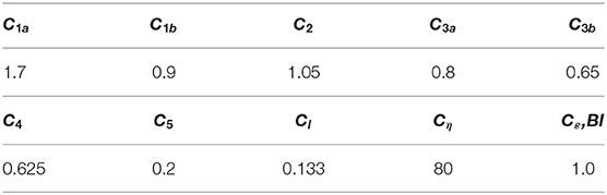
Table 1. Coefficients used in the turbulence model.

Numerical Settings

Numerical simulations were performed using the STAR-CCM+ code (CD-adapco, 2016). For pipe flows, a radial slice of the geometry was considered, whereas a quarter section of the domain was employed for the square duct. At the inlet, constant phase velocities and void fractions were imposed. An isotropic inlet turbulence profile with 2% turbulence intensity was also imposed at the inlet, to facilitate the development toward fully-developed conditions. At the outlet, a fixed pressure boundary condition, and zero gradient conditions on all the other variables, were employed. At the wall, no-slip boundary conditions were enforced on the velocity, with a zero value imposed for the turbulence stresses and the asymptotic limit ε = 2ν (k / y_w)_{yw → 0} used for the turbulence energy dissipation rate. At the wall, the elliptic relaxation function α_EB was set to zero, while a constant value equal to one was imposed at the inlet. On the lateral surfaces of the section, symmetry boundary conditions were imposed on all variables. Convective terms were discretized using second order upwind schemes and the pressure-velocity coupling was solved using a multiphase extension of the SIMPLE algorithm. Simulations were advanced implicitly in time using a second order scheme and, after an inlet development region, fully developed steady-state conditions were reached before recording the results. Strict convergence of residuals as ensured and the mass balance was checked to ensure an error always <0.1 % for both phases.

Grid sensitivity studies ensured that solutions independent of the mesh resolution were reached. Given that significant resolution is needed to properly resolve the near-wall region, the first near-wall cell in the mesh employed was always located at a non-dimensional distance from the wall of y⁺ ~ 1. A sensitivity study is reported in Figure 1 for one of the experiments from Hosokawa and Tomiyama (2009) (experiment H22 in Table 2). Specifically, the figure shows the radial profiles of the water mean velocity, the air void fraction, the radial turbulent stress (responsible for the radial pressure gradient and its impact on the bubble distribution) and the turbulent shear stress. Values are plotted as a function of the non-dimensional radial co-ordinate, which equals 0 in the center of the pipe and 1 at the pipe wall. Three different meshes were tested, having a number of mesh elements equal to 256 × 250 (on the surface perpendicular to the main flow motion and the axial direction, respectively), 420 × 400 and 975 × 750. Both velocity (Figure 1A) and void fraction (Figure 1B) do not show any appreciable difference even from the low to the medium refinement. For the radial normal stress and the turbulent shear stress in Figures 1C,D, some changes are visible from the low to the medium refinement, while no additional differences are found from the medium to the high refinement. Therefore, the mesh with medium refinement (168,000 elements) was used in the simulations. Comparable refinements were used for the other experiments. Given the fact that Hosokawa and Tomiyama (2009) employed a pipe of small diameter, a significantly higher number of elements was necessary for the larger diameter pipes, and 1,280,000 elements were employed for the square duct of Sun et al. (2014) (more details on the specific experiments are provided in the following section).

FIGURE 1

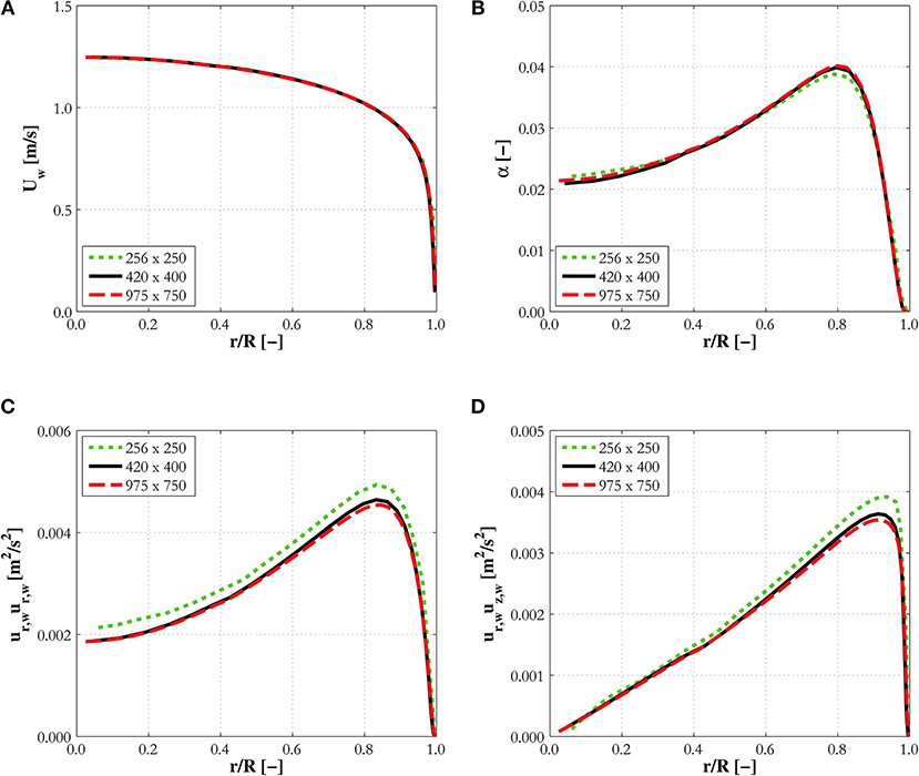
Figure 1. Mesh sensitivity study for experiment H22 from Hosokawa and Tomiyama (2009): (A) water mean velocity; (B) air void fraction; (C) radial turbulent stress; (D) Reynolds shear stress.

TABLE 2

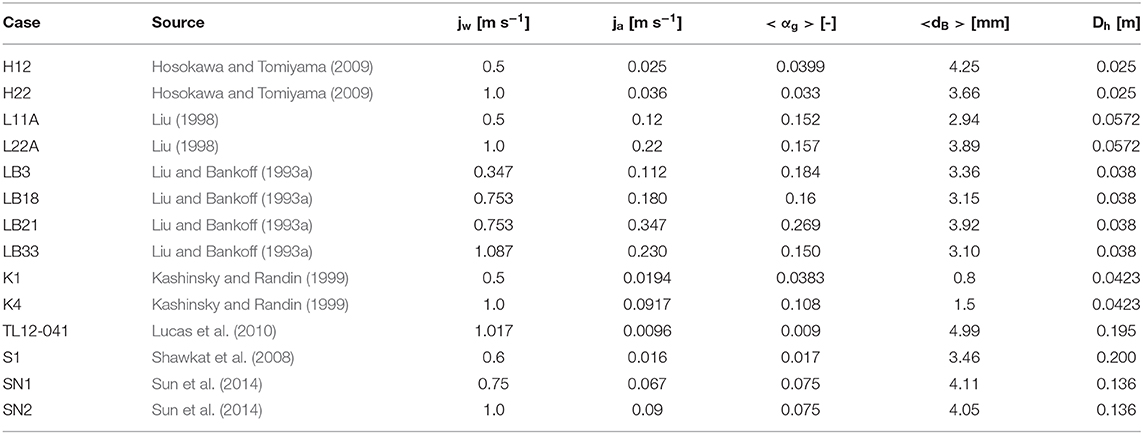
Table 2. Experimental database.

Results and Discussion

Experimental Database

The CFD model will be assessed against a database built using measurements from a number of literature datasets. These includes measurements in vertical upward pipe flows from the works of Liu (1998); Hosokawa and Tomiyama (2009), and Liu and Bankoff (1993a,b) in downward pipe flows from Kashinsky and Randin (1999), in large vertical pipes using the TOPFLOW facility (Shawkat et al., 2008; Lucas et al., 2010), and in a vertical square duct flows (Sun et al., 2014).

The data include a large variety of liquid and gas flow rates, void fractions, bubble diameters and geometries. Since the work described focused on the modeling of multiphase turbulence and interfacial momentum transfer, experiments having as much as possible a monodispersed bubble size distribution were selected as these can be effectively simulated using a constant value of the bubble diameter. Since the present database extends to cases at a high void fraction (for a bubbly flow), it is difficult to assume a monodispersed bubble size distribution in some instances. However, data that showed a marked wall-peaked (in upflow) and core-peaked (in downflow) void fraction profile were selected, allowing the use of a constant lift coefficient. Liquid and gas superficial velocities, and averaged values of the void fraction and the bubble diameter, were used to obtain the correct inlet conditions in the experiments. For the experiments of Liu (1998) and Shawkat et al. (2008), corrections to the nominal gas velocity and averaged void fractions were made from integration of measured radial profiles.

Hosokawa and Tomiyama (2009) measured liquid and gas velocities, void fraction, turbulence in the liquid phase, and bubble number and shape in a vertical upward pipe flow of inside diameter 25 mm. Liu (1998) studied vertical upward flows of air bubbles in water in a pipe of inside diameter 57.2 mm, measuring the liquid velocity, turbulence and the void fraction. In the present simulations, the liquid superficial velocity and the averaged void fraction were imposed, and the latter was used to adjust the gas velocity to achieve the correct flux of air at the measurement position. Liu and Bankoff (1993a) measured liquid and gas velocities, turbulence levels, void fraction and bubble diameter in an upward air-water bubbly flow in a pipe of inside diameter 38 mm. Kashinsky and Randin (1999) measured liquid velocity, turbulence and void fraction in downflow conditions inside a pipe of diameter 42.3 mm. Shawkat et al. (2008) measured upward air-water bubbly flows in a much larger vertical pipe, having a diameter of 200 mm. Liquid and gas velocities and turbulence, void fraction and bubble diameter were measured. A large pipe, having diameter of 195.3 mm, was also used in the TOPFLOW facility (Lucas et al., 2010) to measure bubble size distribution and evolution using the wire-mesh sensor technique. Gas velocity profiles were also measured. Finally, Sun et al. (2014) measured void fraction, bubble diameter and frequency, water velocity and turbulence kinetic energy in a vertical upward bubbly air-water flow in a square duct of side length 136 mm. Details of the experiments are summarized in Table 2. Given that some of the experiments have been used multiple times in previous works [see, for example, Rzehak and Krepper (2015), Rzehak et al. (2017), Parekh and Rzehak (2018), and Magolan and Baglietto (2019)], to reduce confusion and favor consistency we have tried as much as possible to maintain the same naming convention.

Comparison With High-Reynolds Number RSM

In this section, using a first set of simulation results, the EB-RSM predictions are compared with existing results from a previously assessed high-Reynolds number model based on the SSG Reynolds stress model. Details of the model can be found in one of our previous publications (Colombo and Fairweather, 2015). Results are compared against experiments LB18 from Liu and Bankoff (1993a) (Figure 2), H22 from Hosokawa and Tomiyama (2009) (Figure 3) and L22A from Liu (1998) (Figure 4). On the ordinate, the plots show the void fraction, mean liquid (and gas where available) velocity and radial profiles of the turbulence kinetic energy, and the r.m.s. of the velocity fluctuations for Liu and Bankoff (1993a) and Hosokawa and Tomiyama (2009).

FIGURE 2

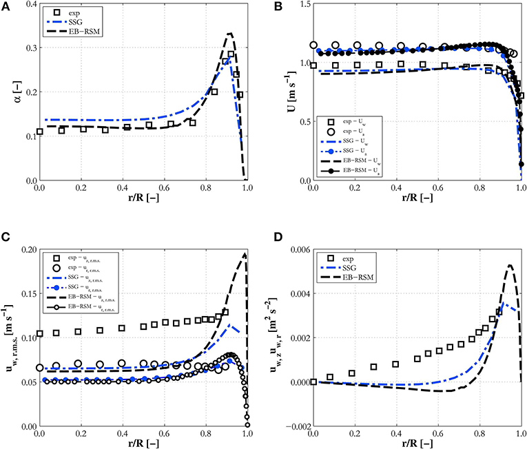
Figure 2. Comparison of EB-RSM simulation results against the SSG model with high-Reynolds number wall treatment for experiment LB18. Radial profiles of: (A) void fraction; (B) water and air mean velocities; (C) axial and radial normal stresses; (D) Reynolds shear stress.

FIGURE 3

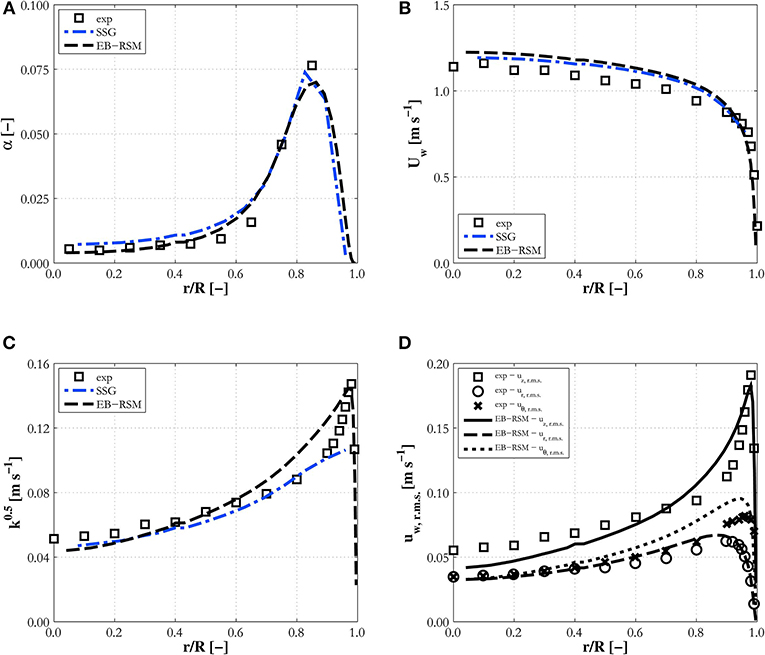
Figure 3. Comparison of EB-RSM simulation results against the SSG model with high-Reynolds number wall treatment for experiment H22. Radial profiles of: (A) void fraction; (B) water mean velocity; (C) turbulence kinetic energy; (D) r.m.s. of water velocity fluctuations (for the EB-RSM only).

FIGURE 4

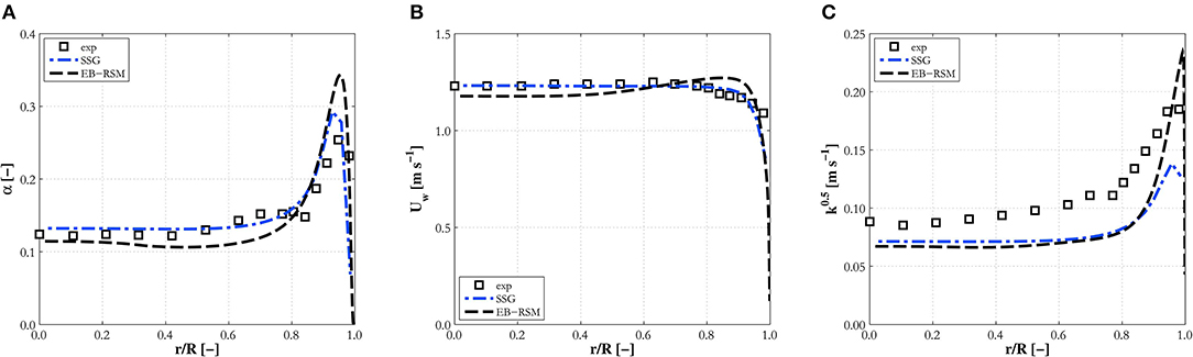
Figure 4. Comparison of EB-RSM simulation results against the SSG model with high-Reynolds number wall treatment for experiment L22A. Radial profiles of: (A) void fraction; (B) water mean velocity; (C) turbulence kinetic energy.

This first comparison serves as an assessment of the capabilities of the EB-RSM compared with a more tested model. The models show similar capabilities and good accuracy. Void fraction profiles (Figures 2A, 3A, 4A) have the typical and expected wall-peaked features and are in very good agreement with the experiments. Most importantly, the magnitude and location of the wall peak are well-predicted by the EB-RSM without the addition of any wall force, and the relative uncertainties connected to a formulation that is, unavoidably, at least partially empirical. This is achieved because, as a consequence of the radial turbulent stress, a radial pressure gradient is generated in the liquid phase and bubbles are pushed toward the pressure minimum in the near-wall region. The radial behavior of the pressure for the three experiments considered is shown in Figure 5. Although the variation in pressure is only a few Pascal, it acts over a few millimeters and is sufficient to affect the bubble distribution and, in the near-wall region, to produce the wall-peaked void fraction profile. Clearly, this pressure gradient, being related to the radial turbulent stress, can only be predicted with accuracy if the anisotropic structure of the turbulence field is accounted for through a Reynolds stress turbulence model, and the near-wall region properly resolved without resorting to wall functions.

FIGURE 5

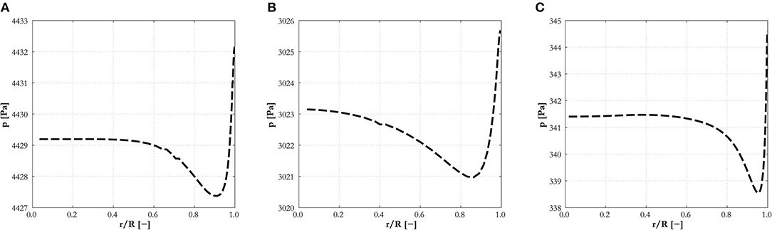
Figure 5. Radial pressure gradient predicted by the EB-RSM for experiments: (A) L18; (B) H22; (C) L22A.

Velocity profiles are also in good agreement with experiments and very similar predictions are found between the two models (Figures 2B, 3B, 4B), although the EB-RSM provides a much more refined resolution in the near-wall region. Turbulence predictions are in agreement with data for Hosokawa and Tomiyama (2009) (Figure 3C) and Liu (1998) (Figure 4C), although both models show discrepancies for Liu and Bankoff (1993a) (Figures 2C,D), for which turbulence levels and the Reynolds shear stress are underpredicted. Additional discussion of these discrepancies will be provided later when predictions with additional data from the same database are presented. It is worth noting here that, while specifically the streamwise, but also the radial, r.m.s. velocities are underpredicted in experiment LB18, much better agreement is found in all three co-ordinate directions for experiment H22 (Figure 3D) from Hosokawa and Tomiyama (2009), proving the models' ability to predict the anisotropic turbulence structure. Away from the wall, predictions from the two models are similar. Near the wall, in contrast, the EB-RSM's higher resolution provides a much improved prediction of the turbulence kinetic energy peak, at least for the cases where turbulence measurements near the wall are available (Figures 3C,D, 4C). In contrast, the SSG model employs a high-Reynolds formulation and wall functions near the wall. For this reason, the first near-wall cell is located at a non-dimensional distance from the wall of y⁺ ~ 30, necessary for the wall function to be valid, and the formulation is not able, as expected, to predict the near-wall peak. Overall, the superior capabilities of the EB-RSM in the near-wall region, and their impact on model predictions, in particular, for the void fraction and turbulence in the fluid phase, suggests that models with near-wall modeling capabilities should be adopted wherever possible. For this reason, only predictions from the EB-RSM will be addressed in the following.

Upward Pipe Flows

In this section, results from the comparisons against the remaining upward pipe flows (excluding large diameter pipes that will be addressed separately) in the database are discussed, and these include the cases from Hosokawa and Tomiyama (2009), Liu and Bankoff (1993a) and Liu (1998). Void fraction profiles were almost always found to be in good agreement with experiments, and Figure 6 provides some examples. Discrepancies are only found in experiment H12 (Figure 6A) in the center of the pipe, and these can be attributed to the presence of some larger bubbles that cannot be predicted using a constant positive value of the lift coefficient. From Hosokawa and Tomiyama (2009), measurements show how a tail of bubbles in the range 6–8 mm is present in the bubble size distribution of this experiment only. The predictions remain accurate at large void fractions, approaching or even exceeding 0.4, such as in experiments LB3 and LB21 (Figure 6B), although for larger liquid velocities (LB33, Figure 6C), the model has a tendency to overpredict the void fraction peak. Overall, the accuracy of the model, even without the addition of any wall force contribution, is encouraging. Clearly, improvements to the lift model, allowing it to predict the change in sign of the lift coefficient, are necessary to extend the overall model's applicability to polydispersed bubbly flows.

FIGURE 6

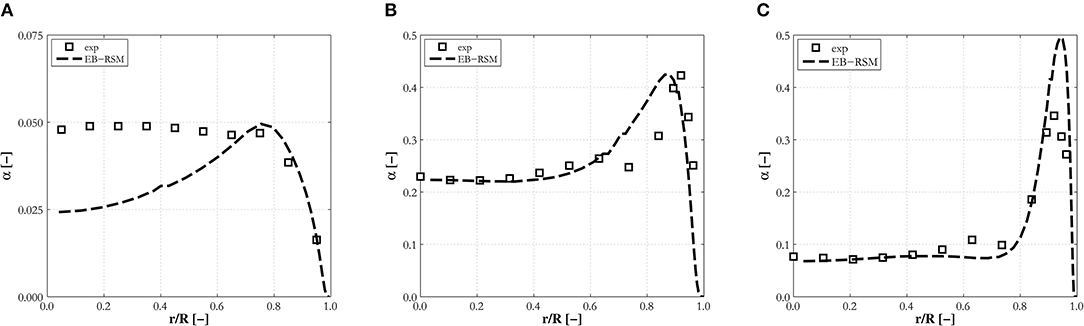
Figure 6. Radial void fraction profiles predicted by the EB-RSM compared against experiments in upward pipe flows: (A) H12; (B) LB21; (C) LB33.

Velocity profiles are in general in good agreement with data, and well-predicted in the very near-wall region (Figure 7A), for cases where the void fraction is not excessively high. At high void fraction, the velocity, driven by bubble buoyancy, tends to peak at the wall (Figures 7B,C), and specific modifications to the drag and near-wall turbulence models might be necessary. Overall, the velocity profiles are almost flat and the slight decrease toward the center of the pipe causes the discrepancies in the prediction of the turbulent shear stress mentioned previously (Figure 2D). It is worth noting that in Liu and Bankoff (1993a) measurements were taken at the shortest distance from the inlet and the turbulent shear stress behavior is not entirely consistent with the close-to-flat velocity profile also observed in the experiments (Figures 2C,D). Additional model testing is therefore desirable, although detailed experimental characterization of the turbulence structure in pipe flows is not frequently found in the literature. The relative velocity, mainly governed by the drag model, tends to be underpredicted on occasion (Figure 7C), contributing to the peak in the liquid velocity profile.

FIGURE 7

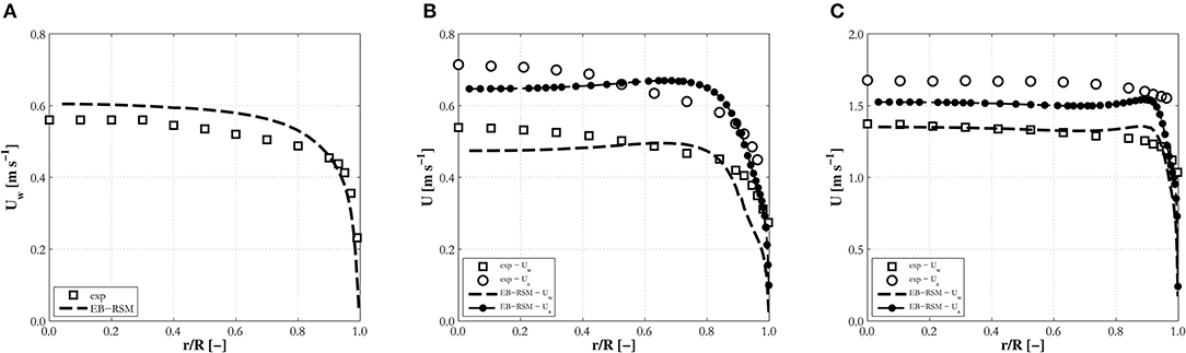
Figure 7. Radial water and air (where available) mean velocity profiles predicted by the EB-RSM compared against experiments in upward pipe flows: (A) H12; (B) LB3; (C) LB33.

Overall, the area in need of most improvement is multiphase turbulence modeling, and the model for bubble-induced turbulence specifically. Although accurate in many cases (Figures 8A, 3C, 4C) discrepancies are found, with the data from Liu and Bankoff (1993a) generally underpredicted (Figure 8C). It is therefore necessary to progress beyond the simple constant values used in the bubble-induced source and the partitioning of this between the different stresses [Equations (13,15)]. Nevertheless, available measurements confirm how the near-wall resolution allows accurate prediction of the peak in the turbulence kinetic energy at the wall (Figures 8A,B).

FIGURE 8

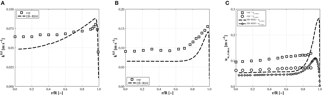
Figure 8. Radial profiles of turbulence kinetic energy, (A,B), and r.m.s. of water velocity fluctuations (C) predicted by the EB-RSM compared against experiments in upward pipe flows: (A) H12; (B) L11A; (C) LB33.

Downward Pipe Flows

This section extends the previous comparisons, limited to upflow cases, to downward flow conditions. In these flows, the bubbles travel at a lower velocity with respect to the liquid phase, and the same lift force pushes them toward the higher relative velocity region that is now in the center of the pipe. This produces core-peaked void fraction profiles, such as those shown in Figures 9A,D for the experiments of Kashinsky and Randin (1999). This behavior is predicted by the model which maintains consistent predictions of the void fraction and shows very good agreement in the near-wall region.

FIGURE 9

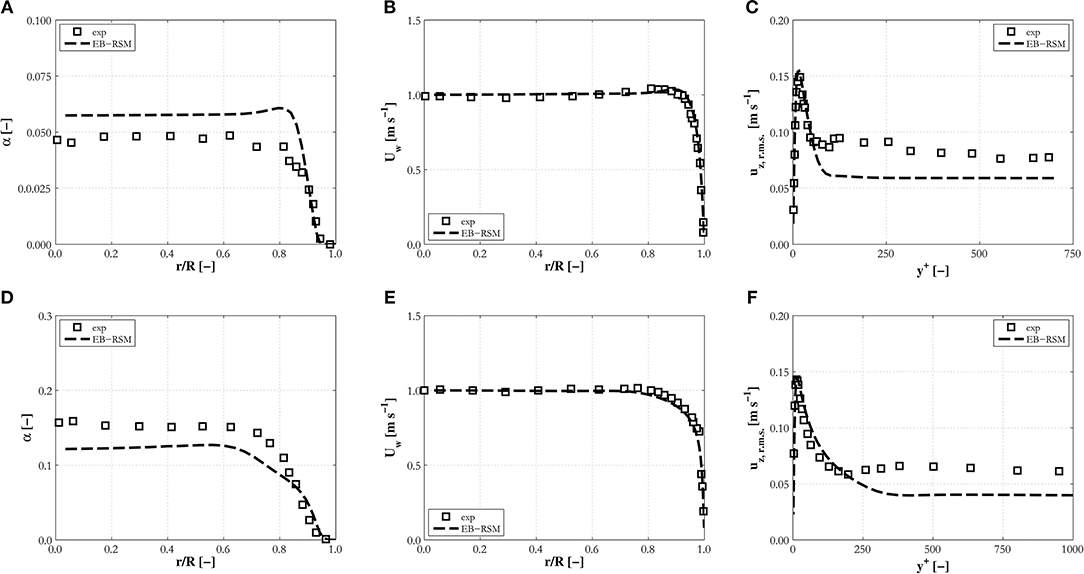
Figure 9. Radial profiles of the void fraction, (A,D), water mean velocity, (B,E), and r.m.s. of axial velocity fluctuations (as a function of the non-dimensional wall distance y⁺), (C,F), predicted by the EB-RSM compared against experiments in downward pipe flows: (A–C) K1; (D–F) K4.

Velocity profiles are in very good agreement (Figures 9B,E), and predictions of the mean velocity and turbulence (Figures 9C,F) are remarkably good in the near-wall region. For these experiments only, the r.m.s. of the streamwise velocity fluctuations is shown as a function of the non-dimensional distance from the wall, in agreement with the way they were originally provided by Kashinsky and Randin (1999). The turbulence intensity is underpredicted by 20–30 % in the center of the pipe. However, in these experiments an additional complication is included since the bubbles have a much smaller diameter than in previous cases, for which the contribution to turbulence from their wakes may become negligible with respect to that due to their random motion. The latter is not properly captured by the type of model used for bubble-induced turbulence in the present work, it being based on the conversion of energy from drag to turbulence kinetic energy in the bubble wakes.

Vertical Pipes of Large Diameter

In previous comparisons, measurements were taken in pipes with diameters of a few centimeters. In the database, two cases with much larger diameter pipes are also included; TL12-041 from the TOPFLOW facility (Lucas et al., 2010) and S1 from Shawkat et al. (2008). These are included to extend the model assessment as much as possible. The pipes considered have diameters of tens of centimeters and their hydrodynamics can be considered to have features similar to those of bubble columns. Wall effects are still present, but their impact extends into the body of the flow much less than in smaller diameter pipes, with uniform velocity and void fraction distributions dominated by mixing found in the bulk of the pipe cross-section. This is clearly evident in the results of Figure 10, where wall effects are confined to the very near-wall region. The model maintains satisfactory agreement with data in these conditions, with the overprediction of the void fraction peak at the wall being the major discrepancy. The air velocity, which has shown some discrepancies in a few previous cases, is instead well-predicted in TL12-041 (Figure 10B). It must also be pointed out that measurements of air velocity and turbulence levels are also available for case S1. However, large and not entirely explicable discrepancies with model predictions have been observed in other studies, for example Parekh and Rzehak (2018), and, for this reason, these data are not included here.

FIGURE 10

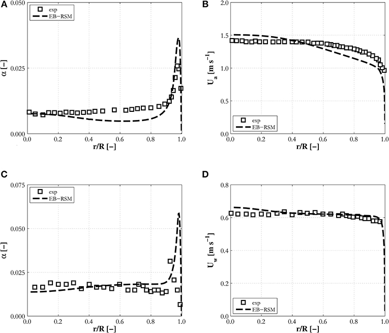
Figure 10. Radial profiles of the void fraction, (A,C), and air (B) and water (D) mean velocities predicted by the EB-RSM compared against experiments in large diameter pipes: (A,B) TL12-041; (C,D) S1.

Square Duct

Finally, predictions are compared against data in a square channel having a relatively large cross sectional area (Sun et al., 2014). In Figures 11, 12, results are shown for three distinct locations, along the diagonal D of the duct, with the abscissa showing the non-dimensional distance from the duct center d / D, and along two lines parallel to the duct wall, one passing through the center of the duct and the other in the near-wall region. For the latter two locations, the abscissa identifies the non-dimensional distance along the line from the center of the duct, x / L. Void fraction behavior has similarities with pipe flows, with the lift force again pushing the bubbles toward the walls of the duct, where the void fraction peaks. Comparing profiles through the duct center from Figures 11B,E with profiles along the wall in Figures 11C,F, it may be noted that the latter are higher, given that they essentially detect the near-wall peak along the wall. The highest values are found in the duct corners, as shown by the peaks along the diagonal in Figures 11A,D, and the line parallel to the near-wall region in Figures 11C,F. The void fraction is well-reproduced by the model for both experiments considered in Figure 11, particularly along the diagonal and the line through the duct center. Some underestimation is found on the line in the near-wall region, although the peak in the duct corner remains well-predicted.

FIGURE 11

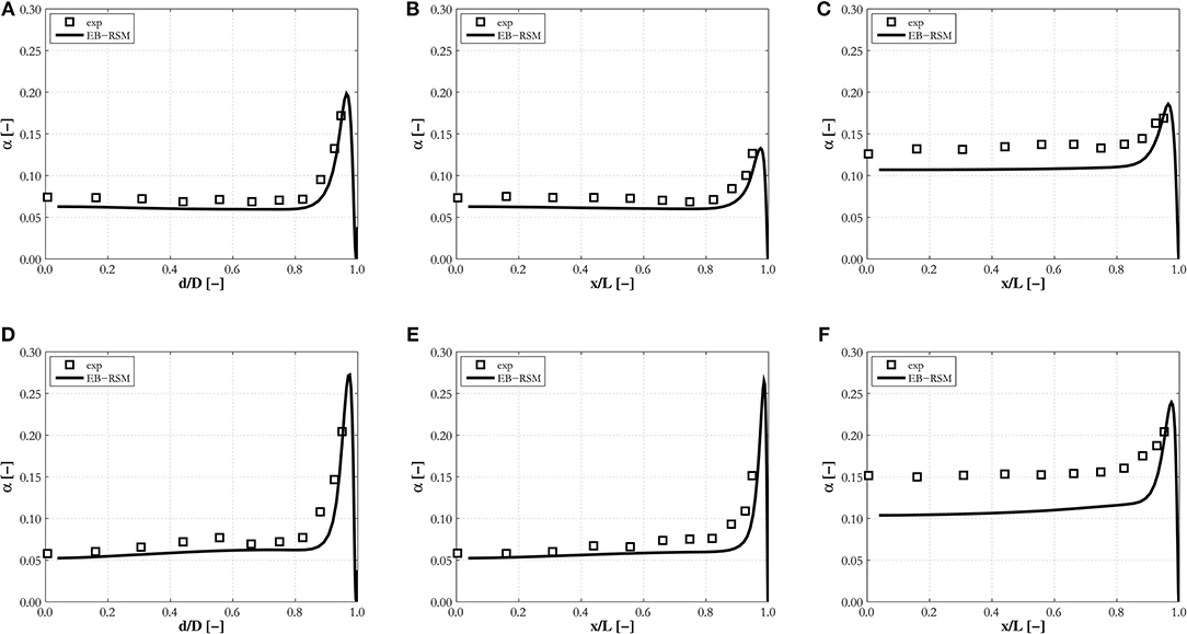
Figure 11. Profiles of the void fraction on the diagonal, (A,D), and a line parallel to the wall passing through the duct center, (B,E), and close to the wall, (C,F), predicted by the EB-RSM compared against Sun et al. (2014) experiments in a square duct: (A–C) SN1; (D–F) SN2.

FIGURE 12

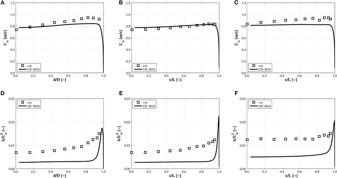
Figure 12. Profiles of the mean liquid velocity and turbulence kinetic energy on the diagonal, (A,D), and a line parallel to the wall passing through the duct center, (B,E), and close to the wall, (C,F), predicted by the EB-RSM compared against Sun et al. (2014) experiments in a square duct: (A–C) SN1; (D–F) SN2.

Lastly, Figure 12 shows mean velocity profiles for experiment SN1 and turbulence kinetic energy, normalized with the square of the mean velocity, for experiment SN2. The qualitative behavior of the velocity, peaking at the walls and corners and slightly decreasing toward the duct center, are well-captured, although the wall-peak is underpredicted. Turbulence levels, in line with previous results, are underestimated in the center of the duct, again confirming remaining challenges in obtaining accurate predictions. In this case, the cross-sectional area is large and the void fraction relatively high, and additional effects promoted by the interaction between bubbles may add to the contribution from their wakes, explaining the underestimation. Peaks in the turbulence kinetic energy are visible at the walls, although the absence of measurements taken in the very near-wall region prevents any comprehensive assessment. Overall, additional model improvements are necessary, but the model performance remains robust even in the square duct geometry.

Conclusions

The performance of an Eulerian-Eulerian multi-fluid CFD model coupled with the EB-RSM turbulence closure, allowing fine resolution of the near-wall region, has been assessed against a large database of air-water bubbly flows. The overall model has demonstrated robust applicability and encouraging accuracy over a wide range of operating conditions and geometrical parameters, with the experimental database including upward and downward pipe flows, large diameter pipe and square duct flows, some of which have rarely, if ever, been tested against.

Good agreement with data for the void fraction distribution was obtained for all experimental cases, with accurate predictions of the magnitude and positon of the near-wall peak found in most experiments. The model does not account for any wall lubrication force, and all the associated uncertainties in modeling this force, and the wall peak is obtained from the action of the radial pressure gradient induced by the turbulence field and its accurate prediction near the wall. In this regard, these results confirm and support recent findings where wall peaked void fraction distributions were also obtained without any wall lubrication effect, as a consequence of which the theoretical basis of the wall lubrication force was questioned. Further evidence will be required, as well as extension to the modeling to handle laminar conditions where turbulent effects are not present, such as with the addition of the turbulent dispersion regularization model of Lubchenko et al. (2018). Overall, and although the lift force remains dominant, these mentioned additional turbulent effects should be taken into account as accurately as possible in any model that aims to be general applicability. For this reason, the transition to models based on Reynolds stress turbulence model formulations, able to capture the anisotropy of the turbulence field, with near-wall resolution capabilities is to be preferred when possible. Such approaches allow fine resolution of the velocity and turbulence field near the wall, although modifications seem necessary at high void fraction given that the elliptic-blending model is still based on its single-phase counterpart. For this to be achieved, the availability of detailed measurements of the turbulent stresses in the near-wall region for further model validation is desirable.

Overall, multiphase turbulence models and the modeling of bubble-induced turbulence are areas in need of major improvement. Over the wide range of conditions tested, multiple physical processes coexist which all contribute in determining a flows' characteristics, which makes predictions particularly challenging. In the short term, more physically based modeling improvements of the bubble-induced source and the attribution of a larger portion of that source to the streamwise direction are necessary. In this regard, some advances have started to appear in the very recent literature (du Cluzeau et al., 2019; Liao et al., 2019).

Finally, it is worth stressing the role of assessments of the kind described for the future development of computational models of bubbly flows. When focusing on only a few experiments for model validation purposes, these can show trends not observable in other cases (see, for example, the differences between Figures 7C, 10B for the air velocity, and Figures 2C, 3D for the turbulence field), and results and modeling improvements should be accepted only when consistent over multiple datasets.

Data Availability Statement

Datasets obtained from the CFD simulations with the EB-RSM for the experiments included in this paper are available at https://doi.org/10.5518/800.

Author Contributions

MC and MF conceived and planned the research, wrote and finalized the manuscript. MC developed the model and performed the simulations.

Conflict of Interest

The authors declare that the research was conducted in the absence of any commercial or financial relationships that could be construed as a potential conflict of interest.

The handling editor declared a past co-authorship with one of the authors MC.

Acknowledgments

The authors gratefully acknowledge the financial support of the EPSRC under grants EP/R021805/1, Can modern CFD models reliably predict DNB for nuclear power applications?, EP/R045194, Computational Modeling for Nuclear Reactor Thermal Hydraulics, and EP/S019871/1, Toward comprehensive multiphase flow modeling for nuclear reactor thermal hydraulics.

References

Antal, S. P., Lahey, R. T., and Flaherty, J. E. (1991). Analysis of phase distribution in fully developed laminar bubbly two-phase flow. Int. J. Multiphase Flow 17, 635–652. doi: 10.1016/0301-9322(91)90029-3

CrossRef Full Text | Google Scholar

Behzadi, A., Issa, R. I., and Rusche, H. (2004). Modelling of dispersed bubble and droplet flow at high phase fractions. Chem. Eng. Sci. 59, 759–770. doi: 10.1016/j.ces.2003.11.018

CrossRef Full Text | Google Scholar

Benhamadouche, S. (2018). On the use of (U)RANS and LES approaches for turbulent incompressible single phase flows in nuclear engineering applications. Nucl. Eng. Des. 312, 2–11. doi: 10.1016/j.nucengdes.2016.11.002

CrossRef Full Text | Google Scholar

Bestion, D. (2014). The difficult challenge of a two-phase CFD modelling for all flow regimes. Nucl. Eng. Des. 279, 116–125. doi: 10.1016/j.nucengdes.2014.04.006

CrossRef Full Text | Google Scholar

Burns, A. D., Frank, T., Hamill, I., and Shi, J. M. (2004). “The Favre averaged drag model for turbulent dispersion in Eulerian multi-phase flows,” in 5th International Conference on Multiphase Flows (Yokohama).

Google Scholar

CD-adapco (2016). STAR-CCM+^® Version 10.04 User Guide.

Google Scholar

Chen, C., Wang, M., Zhao, X., Ju, H., Wang, X., Tian, W., et al. (2019). Numerical study on the single bubble rising behaviors under rolling conditions. Nucl. Eng. Des. 349, 183–192. doi: 10.1016/j.nucengdes.2019.04.039

CrossRef Full Text | Google Scholar

Colombo, M., and Fairweather, M. (2015). Multiphase turbulence in bubbly flows: RANS simulations. Int. J. Multiphase Flow 77, 222–243. doi: 10.1016/j.ijmultiphaseflow.2015.09.003

CrossRef Full Text | Google Scholar

Colombo, M., and Fairweather, M. (2016). RANS simulation of bubble coalescence and break-up in bubbly two-phase flows. Chem. Eng. Sci. 146, 207–225. doi: 10.1016/j.ces.2016.02.034

CrossRef Full Text | Google Scholar

Colombo, M., and Fairweather, M. (2019). Influence of multiphase turbulence modelling on interfacial momentum transfer in two-fluid Eulerian-Eulerian CFD models of bubbly flows. Chem. Eng. Sci. 195, 968–984. doi: 10.1016/j.ces.2018.10.043

CrossRef Full Text | Google Scholar

Daly, B. J., and Harlow, F. H. (1970). Transport equations of turbulence. Phys. Fluids 13, 2634–2649. doi: 10.1063/1.1692845

CrossRef Full Text | Google Scholar

du Cluzeau, A., Bois, G., and Toutant, A. (2019). Analysis and modelling of reynolds stresses in turbuent bubbly up-flows from direct numerical simulations. J. Fluid Mech. 866, 132–168. doi: 10.1017/jfm.2019.100

CrossRef Full Text | Google Scholar

Feng, J., and Bolotnov, I. A. (2017). Evaluation of bubble-induced turbulence using direct numerical simulation. Int. J. Multiphase Flow 93, 92–107. doi: 10.1016/j.ijmultiphaseflow.2017.04.003

CrossRef Full Text | Google Scholar

Feng, J., and Bolotnov, I. A. (2018). Effect of the wall presence on the bubble interfacial forces in a shear flow field. Int. J. Multiphase Flow 99, 73–85. doi: 10.1016/j.ijmultiphaseflow.2017.10.004

CrossRef Full Text | Google Scholar

Gosman, A. D., Lekakou, C., Politis, S., Issa, R. I., and Looney, M. K. (1992). Multidimensional modeling of turbulent two-phase flows in stirred vessels. AIChE J 38, 1946–1956. doi: 10.1002/aic.690381210

CrossRef Full Text | Google Scholar

Hassan, Y. A. (2014). Full-field Measurements of Turbulent Bubbly Flow Using Innovative Experimental Techniques. Technical Report CASL-U-2014-0209-000.

Google Scholar

Hazuku, T., Hibiki, T., and Takamasa, T. (2016). Interfacial area transport due to shear collision of bubbly flow in small-diameter pipes. Nucl. Eng. Des. 310, 592–603. doi: 10.1016/j.nucengdes.2016.10.041

CrossRef Full Text | Google Scholar

Hosokawa, S., Hayashi, K., and Tomiyama, A. (2014). Void distribution and bubble motion in bubbly flows in a 4 × 4 rod bundle. part I: experiments. J. Nucl. Sci. Technol. 51, 220–230. doi: 10.1080/00223131.2013.862189

CrossRef Full Text | Google Scholar

Hosokawa, S., and Tomiyama, A. (2009). Multi-fluid simulation of turbulent bubbly pipe flow. Chem. Eng. Sci. 64, 5308–5318. doi: 10.1016/j.ces.2009.09.017

CrossRef Full Text | Google Scholar

Kashinsky, O. N., and Randin, V. V. (1999). Downward bubbly gas-liquid flow in a vertical pipe. Int. J. Multiphase Flow 25, 109–138. doi: 10.1016/S0301-9322(98)00040-8

CrossRef Full Text | Google Scholar

Lahey, R. T., and Drew, D. A. (2001). The analysis of two-phase flow and heat transfer using a multidimensional, four field, two-fluid model. Nucl. Eng. Des. 204, 29–44. doi: 10.1016/S0029-5493(00)00337-X

CrossRef Full Text | Google Scholar

Lahey, R. T., Jr, Lopez de Bertodano, M., and Jones, O.C., Jr. (1993). Phase distribution in complex geometry conduits. Nucl. Eng. Des. 141, 177–201. doi: 10.1016/0029-5493(93)90101-E

CrossRef Full Text | Google Scholar

Legendre, D., and Magnaudet, J. (1997). A note on the lift force on a spherical bubble or drop in a low-Reynolds-number shear flow. Phys. Fluids 9, 3572–3574. doi: 10.1063/1.869466

CrossRef Full Text | Google Scholar

Lehr, F., Millies, M., and Mewes, D. (2002). Bubble-size distributions and flow fields in bubble columns. AIChE J. 48, 2426–2443. doi: 10.1002/aic.690481103

CrossRef Full Text | Google Scholar

Liao, Y., and Lucas, D. (2009). A literature review of theoretical models for drop and bubble breakup in turbulent dispersions. Chem. Eng. Sci. 64, 3389–3406. doi: 10.1016/j.ces.2009.04.026

CrossRef Full Text | Google Scholar

Liao, Y., and Lucas, D. (2010). A literature review on mechanisms and models for the coalescence process of fluid particles. Chem. Eng. Sci. 65, 2851–2864. doi: 10.1016/j.ces.2010.02.020

CrossRef Full Text | Google Scholar

Liao, Y., Ma, T., Krepper, E., Lucas, D., and Frohlich, J. (2019). Application of a novel model for bubble-induced turbulence to bubbly flows in containers and vertical pipes. Chem. Eng. Sci. 202, 55–69. doi: 10.1016/j.ces.2019.03.007

CrossRef Full Text | Google Scholar

Liao, Y., Ma, T., Liu, L., Ziegenhein, T., Krepper, E., and Lucas, D. (2018). Eulerian modelling of turbulent bubbly flow based on a baseline closure concept. Nucl. Eng. Des. 337, 450–459. doi: 10.1016/j.nucengdes.2018.07.021

CrossRef Full Text | Google Scholar

Liao, Y., Rzehak, R., Lucas, D., and Krepper, E. (2015). Baseline closure model for dispersed bubbly flow: bubble coalescence and breakup. Chem. Eng. Sci. 122, 336–349. doi: 10.1016/j.ces.2014.09.042

CrossRef Full Text | Google Scholar

Liu, H., and Hibiki, T. (2018). Bubble breakup and coalescence models for bubbly flow simulation using interfacial area transport equation. Int. J. Heat Mass Tran. 126, 128–146. doi: 10.1016/j.ijheatmasstransfer.2018.05.054

CrossRef Full Text | Google Scholar

Liu, T. J. (1998). “The role of bubble size on liquid phase turbulent structure in two-phase bubbly flow,” in 3rd International Conference on Multiphase Flow (ICMF1998) (Lyon).

Google Scholar

Liu, T. J., and Bankoff, S. G. (1993a). Structure of air-water bubbly flow in a vertical pipe—I. liquid mean velocity and turbulence measurements. Int. J. Heat Mass Tran. 36, 1049–1060. doi: 10.1016/S0017-9310(05)80289-3

CrossRef Full Text | Google Scholar

Liu, T. J., and Bankoff, S. G. (1993b). Structure of air-water bubbly flow in a vertical pipe—II. void fraction, bubble velocity and bubble size distribution. Int. J. Heat Mass Tran. 36, 1061–1072. doi: 10.1016/S0017-9310(05)80290-X

CrossRef Full Text | Google Scholar

Lopez de Bertodano, M., Lahey, R. T., and Jones, O. C. (1994). Phase distribution in bubbly two-phase flow in vertical ducts. Int. J. Multiphase Flow 20, 805–818. doi: 10.1016/0301-9322(94)90095-7

CrossRef Full Text | Google Scholar

Lopez de Bertodano, M., Lee, S. J., Lahey, R. T. Jr., and Drew, D.A. (1990). The prediction of two-phase turbulence and phase distribution phenomena using a reynolds stress model. J. Fluid Eng. 112, 107–113. doi: 10.1115/1.2909357

CrossRef Full Text | Google Scholar

Lu, J., and Tryggvason, G. (2013). Dynamics of nearly spherical bubbles in a turbulent channel upflow. J. Fluid Mech. 732, 166–189. doi: 10.1017/jfm.2013.397

CrossRef Full Text | Google Scholar

Lubchenko, N., Magolan, B., Sugrue, R., and Baglietto, E. (2018). A more fundamental wall lubrication force from turbulent dispersion regularization for multiphase CFD applications. Int. J. Multiphase Flow 98, 36–44. doi: 10.1016/j.ijmultiphaseflow.2017.09.003

CrossRef Full Text | Google Scholar

Lucas, D., Beyer, M., Szalinski, L., and Schutz, P. (2010). A new databse on the evolution of air-water flows along a large vertical pipe. Int. J. Therm. Sci. 49, 664–674. doi: 10.1016/j.ijthermalsci.2009.11.008

CrossRef Full Text | Google Scholar

Lucas, D., Krepper, E., and Prasser, H. M. (2005). Development of co-current air-water flow in a vertical pipe. Int. J. Multiphase Flow 31, 1304–1328. doi: 10.1016/j.ijmultiphaseflow.2005.07.004

CrossRef Full Text | Google Scholar

Lucas, D., Rzehak, R., Krepper, E., Ziegenhein, T., Liao, Y., Kriebitzsch, P., et al. (2016). A strategy for the qualification of multi-fluid approaches for nuclear reactor safety. Nucl. Eng. Des. 299, 2–11. doi: 10.1016/j.nucengdes.2015.07.007

CrossRef Full Text | Google Scholar

Ma, T., Santarelli, C., Ziegenhein, T., Lucas, D., and Frohlich, J. (2017). Direct numerical simulation-based reynolds-averaged closure for bubble-induced turbulence. Phys. Rev. Fluids 2:034301. doi: 10.1103/PhysRevFluids.2.034301

CrossRef Full Text | Google Scholar

Magolan, B., and Baglietto, E. (2019). Assembling a bubble-induced turbulence model incorporating physcial understanding from DNS. Int. J. Multiphase Flow 116, 185–202. doi: 10.1016/j.ijmultiphaseflow.2019.04.009

CrossRef Full Text | Google Scholar

Magolan, B., Baglietto, E., Brown, C., Bolotnov, I. A., Tryggvason, G., and Lu, J. (2017). Multiphase turbulence mechanisms identification from consistent analysis of direct numerical simulation data. Nucl. Eng. Technol. 49, 1318–1325. doi: 10.1016/j.net.2017.08.001

CrossRef Full Text | Google Scholar

Manceau, R. (2015). Recent progress in the development of the elliptic blending reynolds-stress model. Int. J. Heat Fluid Flow 51, 195–220. doi: 10.1016/j.ijheatfluidflow.2014.09.002

CrossRef Full Text | Google Scholar

Manceau, R., and Hanjalic, K. (2002). Elliptic blending model: a new near-wall reynolds-stress turbulence closure. Phys. Fluids 14, 744–754. doi: 10.1063/1.1432693

CrossRef Full Text | Google Scholar

Martinez-Bazan, C., Montanes, J. L., and Lasheras, J. C. (1999). On the breakup of an air bubble injected into a fully developed turbulent flow. part 1. breakup frequency. J. Fluid Mech. 401, 157–182. doi: 10.1017/S0022112099006680

CrossRef Full Text | Google Scholar

Mehrabani, M. T., Nobari, M. R. H., and Tryggvason, G. (2017). An efficient front-tracking method for simulation of multi-density bubbles. Int. J. Numer. Methods Flow 84, 445–465. doi: 10.1002/fld.4355

CrossRef Full Text | Google Scholar

Mimouni, S., Archambeau, F., Boucker, M., Lavieville, J., and Morel, C. (2010). A second order turbulence model based on a reynolds stress approach for two-phase boiling flows. part 1: application to the ASU-annular channel case. Nucl. Eng. Des. 240, 2233–2243. doi: 10.1016/j.nucengdes.2009.11.019

CrossRef Full Text | Google Scholar

Mimouni, S., Baudry, C., Guingo, M., Hassanaly, M., Lavieville, J., Mechitoua, N., et al. (2015). “Combined evaluation of bubble dynamics, polydispersion model and turbulence modelling for adiabatic two-phase flow,” in 16th International Topical Meeting on Nucelar Reactor Thermal-Hydraulics (NURETH-16) (Chicago, IL).

Google Scholar

Mimouni, S., Guingo, M., Lavieville, J., and Merigoux, N. (2017). Combined evaluation of bubble dynamics, polydispersion model and turbulence modeling for adiabatic two-phase flow. Nucl. Eng. Des. 321, 57–68. doi: 10.1016/j.nucengdes.2017.03.041

CrossRef Full Text | Google Scholar

Parekh, J., and Rzehak, R. (2018). Euler-Euler multiphase CFD-simulation with full Reynolds stress model and anisotropic bubble-induced turbulence. Int. J. Multiphase Flow 99, 231–245. doi: 10.1016/j.ijmultiphaseflow.2017.10.012

CrossRef Full Text | Google Scholar

Podowski, M. Z. (2018). Is reactor multiphase thermal-hydraulics a mature field of engineering science? Nucl. Eng. Des. 345, 196–208. doi: 10.1016/j.nucengdes.2019.01.022

CrossRef Full Text | Google Scholar

Politano, M. S., Carrica, P. M., and Converti, J. (2003). A model for turbulent polydisperse two-phase flow in vertical channels. Int. J. Multiphase Flow 29, 1153–1182. doi: 10.1016/S0301-9322(03)00065-X

CrossRef Full Text | Google Scholar

Prince, M. J., and Blanch, H. W. (1990). Bubble coalescence and breakup in air-sparged bubble columns. AIChE J. 36, 1485–1499. doi: 10.1002/aic.690361004

CrossRef Full Text | Google Scholar

Risso, F. (2018). Agitation, mixing and transfers induced by bubbles. Annu. Rev. Fluid Mech. 50, 25–48. doi: 10.1146/annurev-fluid-122316-045003

CrossRef Full Text | Google Scholar

Rzehak, R., and Krepper, E. (2013). CFD modeling of bubble-induced turbulence. Int. J. Multiphase Flow 55, 138–155. doi: 10.1016/j.ijmultiphaseflow.2013.04.007

CrossRef Full Text | Google Scholar

Rzehak, R., and Krepper, E. (2015). Bubbly flows with fixed polydispersity: validation of a baseline closure model. Nucl. Eng. Des. 287, 108–118. doi: 10.1016/j.nucengdes.2015.03.005

CrossRef Full Text | Google Scholar

Rzehak, R., Krepper, E., and Lifante, C. (2012). Comparative study of of wall-force models for the simulation of bubbly flows. Nucl. Eng. Des. 253, 41–49. doi: 10.1016/j.nucengdes.2012.07.009

CrossRef Full Text | Google Scholar

Rzehak, R., Ziegenhein, T., Kriebitzsch, P., Krepper, E., and Lucas, D. (2017). Unified modelling of bubbly flows in pipes, bubble columns, and airlift columns. Chem. Eng. Sci. 157, 147–158. doi: 10.1016/j.ces.2016.04.056

CrossRef Full Text | Google Scholar

Santarelli, C., and Frohlich, J. (2015). Direct numerical simulations of spherical bubbles in vertical turbulent channel flow. Int. J. Multiphase Flow 75, 174–193. doi: 10.1016/j.ijmultiphaseflow.2015.05.007

CrossRef Full Text | Google Scholar

Santarelli, C., and Fröhlich, J. (2016). Direct numerical simulations of spherical bubbles in vertical turbulent channel flow. Influence of bubble size and bidispersity. Int. J. Multiphase Flow 81, 27–45. doi: 10.1016/j.ijmultiphaseflow.2016.01.004

CrossRef Full Text | Google Scholar

Shaver, D. R., and Podowski, M. Z. (2015). Modeling of interfacial forces for bubbly flows in subcooled boiling conditions. Trans. Am. Nucl. Soc. 113, 1368–1371.

Google Scholar

Shawkat, M., Ching, C., and Shoukri, M. (2008). Bubble and liquid turbulence characteristics of bubbly flow in a large diameter vertical pipe. Int. J. Multiphase Flow 34, 767–785. doi: 10.1016/j.ijmultiphaseflow.2008.01.007

CrossRef Full Text | Google Scholar

Speziale, C. G., Sarkar, S., and Gatski, T. B. (1991). Modelling the pressure-strain correlation of turbulence: an invariant dynamical system approach. J. Fluid Mech. 227, 245–272. doi: 10.1017/S0022112091000101

CrossRef Full Text | Google Scholar

Sugrue, R., Magolan, B., Lubchenko, N., and Baglietto, E. (2017). Assessment of a simplified set of momentum closure relations for low volume fraction regimes in STAR-CCM+ and OpenFOAM. Ann. Nucl. Energy 110, 79–87. doi: 10.1016/j.anucene.2017.05.059

CrossRef Full Text | Google Scholar

Sun, H., Kunugi, T., Shen, X., Wu, D., and Nakamura, H. (2014). Upward air-water bubbly flow characteristics in a vertical square duct. J. Nucl. Sci. Technol. 51, 267–281. doi: 10.1080/00223131.2014.863718

CrossRef Full Text | Google Scholar

Tomiyama, A., Celata, G. P., Hosokawa, S., and Yoshida, S. (2002a). Terminal velocity of single bubbles in surface tension dominant regime. Int. J. Multiphase Flow 28, 1497–1519. doi: 10.1016/S0301-9322(02)00032-0

CrossRef Full Text | Google Scholar

Tomiyama, A., Tamai, H., Zun, I., and Hosokawa, S. (2002b). Transverse migration of single bubbles in simple shear flows. Chem. Eng. Sci. 57, 1849–1858. doi: 10.1016/S0009-2509(02)00085-4

CrossRef Full Text | Google Scholar

Troshko, A. A., and Hassan, Y. A. (2001). A two-equation turbulence model of turbulent bubbly flows. Int. J. Multiphase Flow 27, 1965–2000. doi: 10.1016/S0301-9322(01)00043-X

CrossRef Full Text | Google Scholar

Ullrich, M., Maduta, R., and Jakirlic, S. (2014). “Turbulent bubbly flow in a vertical pipe computed by an eddy-resolving reynolds stress model,” 10th International ERCOFTAC Symposium on Engineering Turbulence Modelling and Measurements (ETMM 10) (Marbella).

Google Scholar

Wang, S. K., Lee, S. J., Jones, O. C., and Lahey, R. T. (1987). 3-D turbulence structure and phase distribution measurements in bubbly two-phase flows. Int. J. Multiphase Flow 13, 327–343. doi: 10.1016/0301-9322(87)90052-8

CrossRef Full Text | Google Scholar

Welleck, R. M., Agrawal, A. K., and Skelland, A. H. P. (1966). Shape of liquid drops moving in liquid media. AIChE J. 12, 854–862. doi: 10.1002/aic.690120506

CrossRef Full Text | Google Scholar

Yao, W., and Morel, C. (2004). Volumetric interfacial area prediction in upward bubbly two-phase flow. Int. J. Heat Mass Tran. 47, 307–328. doi: 10.1016/j.ijheatmasstransfer.2003.06.004

CrossRef Full Text | Google Scholar

Yeoh, G. H., and Tu, J. Y. (2006). Two-fluid and population balance models for subcooled boiling flow. Appl. Math. Model. 30, 1370–1391. doi: 10.1016/j.apm.2006.03.010

CrossRef Full Text | Google Scholar