Analysis of Harmonic Resonance for Locomotive and Traction Network Interacted System Considering the Frequency-Domain Passivity Properties of the Digitally Controlled Converter

Harmonic resonance is a kind of oscillatory instability phenomenon occurring in the electric railway. To investigate this problem, the frequency-domain model of the single-phase voltage source converter for locomotives is derived based on the transfer function of the current control loop. The equivalent circuit of the traction network is also included in this frequency-domain model. Particularly, the time delay and zero-order-holder effect of the digital pulse width modulation are taken into consideration in order to obtain more accurate a model of the digital controller. After that, the harmonic resonance of the locomotive-network system is assessed through the passivity properties of the interacted frequency-domain impedance model. Finally, the effectiveness of the theoretical analysis is demonstrated by simulations and experiments. As a result, the harmonic resonance can be predicted before a new electric railway is put into use so that some mitigation measures can be taken in advance.

Introduction

In electric railways, lots of power electronic converters are applied to high-power locomotives and electric multiple units (hereafter, all referred to locomotives) with an AC-DC-AC traction drive system. The traction network provides electric power for locomotives, which forms a single-phase interacted L-N system. Multiple-loop digital controllers for converters of locomotives are designed for regulating the current and the power which are drawn from the traction network. The control dynamics can destabilize the L-N system when the controller presents poor damping at the harmonic resonance frequency of the traction network (Song et al., 2016). Some harmonic resonance accidents have occurred on different electric railways, resulting in the breakdown of the high-voltage equipment, the erroneous operation of the protective devices, even the traction blockades of the locomotives (Cui et al., 2015). The destroyed arresters are illustrated in Figure 1. Therefore, it is necessary to investigate the stability of the L-N system in order to mitigate the harmonic resonance on electric railways.

FIGURE 1

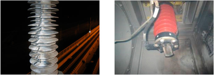
FIGURE 1. The high-voltage equipment destroyed by the harmonic resonance.

It is not sufficient to regard the VSC as a harmonic source for the research on the harmonic resonance of the L-N system because of the various characteristics of the harmonic current for different L-N systems. To explore the mechanism of the harmonic resonance, the VSC is generally considered as a harmonic current source (Lee et al., 2006). The traction network is modeled as a harmonic resonance circuit (Kolar et al., 2010). The harmonic spectra of the AC side current can be derived by applying the Fourier transform to the pulse width modulation (PWM) (Mouton et al., 2014; Kostic et al., 2013). Several inherent harmonic resonance frequencies exist according to the impedance-frequency characteristics of the traction network (Holtz and Kelin, 1989; Zhang et al., 2017; Qiujiang et al., 2018). The harmonic current generated by the VSC flows into the traction network through the point-of-common-coupling (PCC) for the L-N system (Tan et al., 2005). Some harmonic current components will be amplified when the frequency of the harmonic current corresponds to the inherent resonance frequency of the traction network (Song et al., 2017). However, the harmonic spectra of the ac side voltage and current are influenced by not only the PWM but also the performance of the controller. Moreover, the frequency ranges of harmonic resonance accidents differ for various railway lines and locomotives (Song et al., 2019).

Then, the integrated model of the traction network and the VSC is convenient to analyze the stability of the L-N system. The frequency-domain modeling of the VSC and the traction network is widely investigated to probe into their influence on the stability of the interacted system. The dq-domain impedance matrix, the αβ-domain impedance matrix, and the sequence-domain impedance of the VSC controller are established by the small-signal method (Rygg et al., 2016; Wang et al., 2018; Li et al., 2019; Zhang et al., 2019b). The multi-conductor transmission line model is the popular equivalent of the traction network (Mingli et al., 2010; Liu et al., 2016). However, the electric railway is a single-phase system, so it is not convenient to model the locomotive VSC controller in a dq-frame, αβ-frame, or sequence-domain. In addition, the impedance of the power source also has a non-negligible influence on the impedance of the VSC controller (Zhang et al., 2019a). Therefore, the frequency-domain model of the VSC including the parameters of the traction network is beneficial to the comprehensive analysis of the L-N system.

More importantly, the time delay and the zero-order-holder (ZOH) effect of the digital pulse width modulation (DPWM) should be taken into consideration for the modeling of the integrated model. Furthermore, the time delay is a common phenomenon in digital control systems (Nguyen et al., 2020). The dynamic performance of the digital controllers of the power electronics plays an important role in the harmonic resonance for the electronic device penetrated source-load system (Harnefors et al., 2008). With the rapid development of the microprocessors, such as the digital-signal processor (DSP), and the field-programmable gate-array (FPGA) and so on, the digital controllers have been widely used in the control of the power electronic device (Buso and Mattavelli, 2006; Dorf and Bishop, 2016). Generally, the central controller plus the distributed controllers are adopted in the digital controller of the multi-VSCs system (Wu and Mingli, 2017). Also, the DPWM is implemented by updating the modulation reference at the peaks of the triangle carrier, which is called asymmetrically sampled PWM (ASPWM) (Buso and Mattavelli, 2006; Mouton et al., 2014). Some novel DPWM methods even adopt the multi-sampling method and the modulation signal is updated several times within one period of the carrier in order to reduce the control delay of the PWM process (Castro & et al., 2003; Yang & et al., 2019). Thus, various time delays are introduced to the digital controller, which needs to be considered when establishing the frequency-domain model of the VSC controller. However, the time delay and the ZOH effect of the DPWM are neglected or simplified in some cases. This approach may lead to an inaccurate assessment of system stability.

Based on the frequency-domain model of the digital controller including the DPWM, the harmonic resonance of the L-N system can be assessed by the stability criteria. The stability of the L-N system is generally studied by applying the stability criteria to the frequency-domain model (Amin and Molinas, 2017). Passivity-based stability is an effective approach to analyze the harmonic resonance issues (Paice and Meyer, 2000; Harnefors et al., 2016). Namely, the positive real part of the system impedance for all frequencies indicates that the system can be guaranteed to be stable (Sainz et al., 2017). The real part of the impedance is determined by not only the time delay and the ZOH effect of the DPWM but also the traction network. Because of the performance of the digital controller and the characteristics of the traction network, the positive real part of the system impedance cannot always be satisfied for the whole frequency range. So these criteria can be extended to a limited frequency range of the passive property (Harnefors et al., 2007). There does not exist the risk of the resonance amplification when the inherent resonance frequency locates in the frequency range of the passive region.

This paper attempts to assess the stability of the L-N system by taking the computational delay and the DPWM into consideration. The contributions of the paper are:

a. The total impedance model of the L-N system is derived by combining the impedance of the traction network with the current controller of the converter.

b. The influence of the computation delay and the DPWM on the harmonic resonance of the L-N impedance is investigated by the passivity properties of the total impedance model.

c. The harmonic resonance can be predicted based on the frequency-domain passivity of the total impedance before a new electric railway is put into use.

The rest of the paper is organized as follows. The onsite measurement of the harmonic resonance is given in “Onsite Measurement of the Harmonic Resonance”. In “System Modeling” , the frequency-domain model of the L-N system is derived by taking the current controller and the DPWM into consideration. Afterward, the theoretical analysis, the time-domain simulation, and the experiments are conducted in “Stability Analysis and Verification.” Finally, “Conclusions” concludes this paper.

Onsite Measurement of the Harmonic Resonance

In an electric railway, a railway line is divided into several power supply sections (PSSs) through the section posts (SPs). When the locomotive moves in different PSSs or different locomotives move in the same PSS, the electrical property of the interacted system presents various characteristics. Therefore, the harmonic resonance tends to occur suddenly in one PSS and then gradually vanishes as the locomotive runs into another PSS. Moreover, in one PSS, the harmonic resonance happens only when certain types of locomotive run.

Figure 2 displays the onsite measurement data obtained in the traction substation (SS) of the railway line. The voltage signal is sampled from the secondary winding of the Scott traction transformer and the current is sampled from one of the feeders. As depicted in Figures 2A,B, the current and the voltage are relatively pure and sinusoidal. Then the harmonic resonance is triggered so that the current and the voltage are distorted as shown in Figures 2C,D. The harmonic resonance lasts for 298 s. After that, the electric railway goes back to the ordinary operation condition.

FIGURE 2

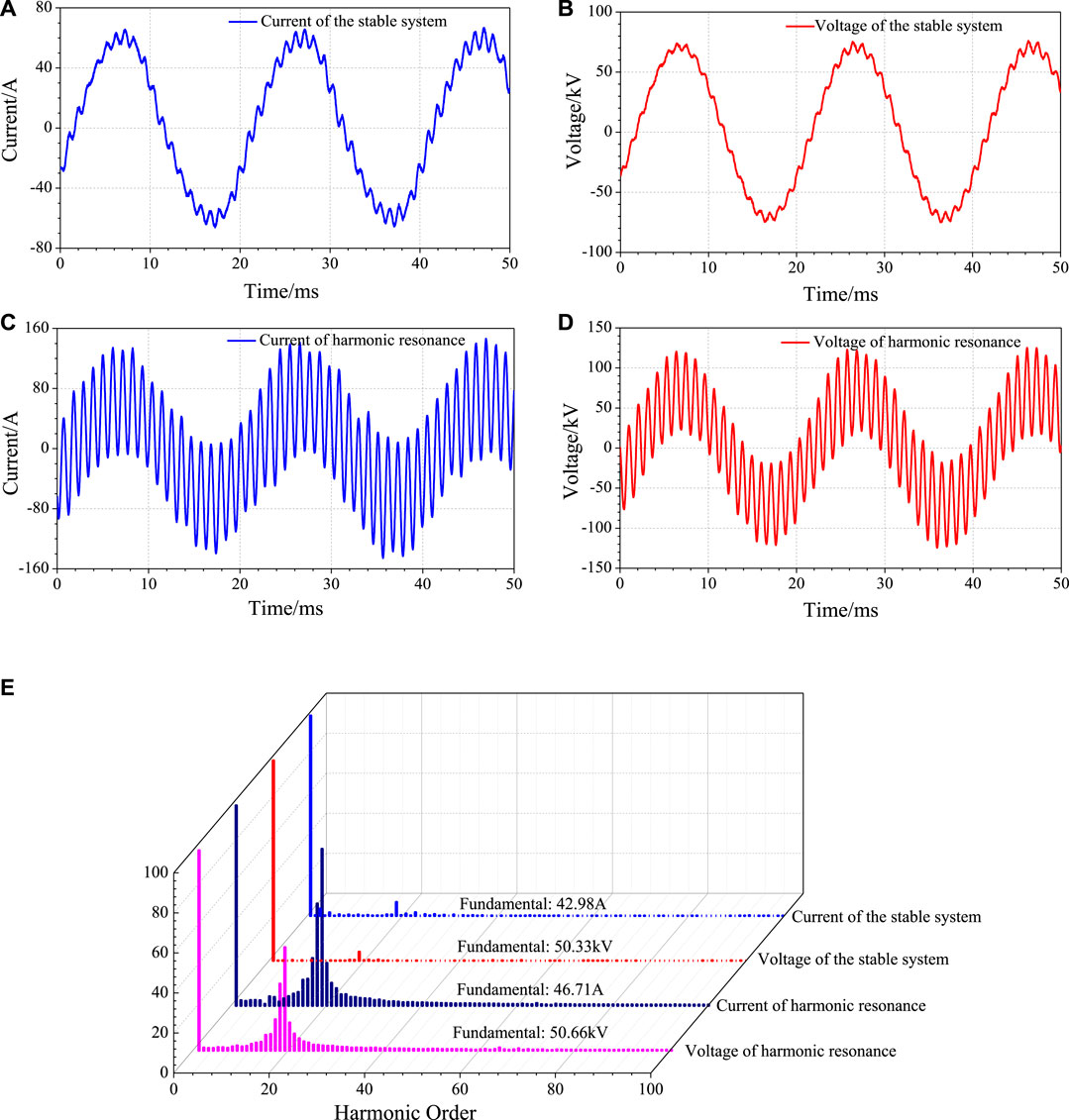
FIGURE 2. The waveforms of current and voltage (A) current of the stable system (B) voltage of the stable system (C) current of harmonic resonance (D) voltage of harmonic resonance. (E) The harmonic spectra of the current and voltage.

The harmonic content of the current and the voltage is analyzed by Fast Fourier Transformation (FFT). Figure 2E presents the harmonic spectra. Obviously, in the normal state, all of the current harmonic content is not higher than 6.8% (6.8%, the 19th current harmonic content) and all of the voltage harmonic content is not higher than 4.4% (4.4%, the 19th voltage harmonic content). However, when the harmonic resonance happens, the 19th (950 Hz) current harmonic content is up to 78.2% while the voltage harmonic content of the same frequency is up to 51.6%. Although the fundamental current and voltage do not increase much, the over-voltage is excited in the railway because of the harmonic amplification. The root mean square value (RMS) voltage of the traction network is as high as 65 kV, which exceeds the maximum short-term allowable voltage of the AT traction network, 58 kV. Therefore, the harmonic resonance is the instability problem which is related to both the locomotive and the power supply system.

System Modeling

System Description of the Locomotive-Network System

The locomotive draws electricity from the power supply system by the onboard traction drive system. The single-phase four-quadrant VSC of the locomotive plays an important role in converting the single-phase electricity into the three-phase electricity which is needed by the traction motor. Therefore, the matching characteristics of the locomotive and the power supply system mainly depend on the VSC and the traction network. As a result, the model of the locomotive can be simplified as the VSC model.

As shown in Figure 3A, the traction drive system of the locomotive contains the single-phase VSC, three-phase inverter, and the traction motor. The onboard transformer of the locomotive is equivalent to the inductance (L_t) in series with the resistance (R_t). The double closed-loop controller of the VSC is illustrated in Figure 3B. The ac current from the VSC is regulated through the inner current controller (CC) in order to maintain the current and the voltage in the same phase. The DC voltage outer loop controller (VC) provides the amplitude reference value for the CC. Then the sinusoidal current reference of the CC is generated through the synchronization with the line voltage by the phase lock loop (PLL). Then the CC outputs the modulation wave for PWM. The insulated gate bipolar transistors (IGBTs) of the VSC are on/off by PWM pulses. The DC voltage keeps stable by the VC.

FIGURE 3

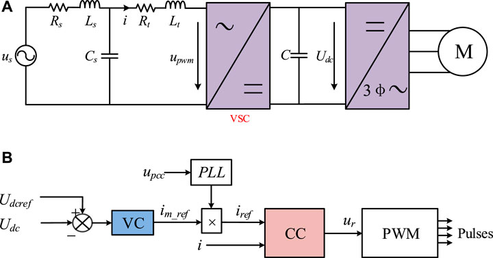
FIGURE 3. The illustration of the L-N system and the controller of the VSC. (A) The simplified one-line diagram. (B) the double closed-loop controller of the VSC.

The three-phase inverter transforms the stable dc voltage into the three-phase ac voltage according to the power of the motor. The inverter can be equivalent to the load of the converter and the DC voltage is the power source of the inverter. The power of the locomotive determines the input power of the converter. The voltage of the DC link remains stable when the input power of the converter changes. As a result, the DC source of the inverter is stable. Therefore, the three-phase inverter and the traction motor are not included in the locomotive modeling for the stability assessment of the L-N system.

For the double closed-loop controller, the bandwidth of the outer loop is lower than that of the inner loop (Buso and Mattavelli, 2006). As a consequence, for the controller of the VSC, the bandwidth of the CC is higher than that of the VC. Because of the low bandwidth, the outer voltage loop mainly influences he impedance-frequency characteristic in the low-frequency range (below 2f₀, f₀ is the fundamental frequency) and it contributes little to the instability phenomenon of the high-frequency range (from 2f₀ to f_sa/2, f_sa is the sampling frequency of the controller). The constant DC voltage and the current reference are assumed when the harmonic instability is investigated. Therefore, for the purpose of analyzing the harmonic resonance through the simplified model, only the frequency-domain characteristics of the CC are considered.

In addition, the power supply system, including the traction network, is equivalent as the series inductance (L_s) and the shunt capacitance (C_s) (Liu et al., 2016). These two parameters vary with the location of the locomotive. The traction network is a complex system with distributed parameters. For the two main traction network topologies, the direct feeding system with return wire (T-R + NF) and the auto-transformer (AT) feeding system, the impedance-frequency characteristic are nearly the same. Therefore, the traction network topology is not clarified in the model.

Model of the Digital Pulse Width Modulation for the Locomotive

The DPWM is implemented in the digital control chip by comparing this modulation reference and the triangle carrier. The CC outputs the modulation reference of the DPWM process. The DPWM process is illustrated in Figure 4. As shown in Figure 4A, the modulation signal in the continuous system is a sinusoidal wave. Nevertheless, in the digital control, the modulation wave is updated immediately at the peak (including the negative peak and the positive peak) of the triangle carrier so that it is not a continuous signal but a discrete signal. The sample period is represented as T_s. Both the sample and the controller calculation are not taken into consideration. The DPWM is similar to the sampling of the ideal modulation wave. So the DPWM can be modeled as a ZOH element. Thus, the transfer function of the VSC ac voltage to modulation reference is obtained:

$G_{pwma}\left(s\right)=\frac{1-e^{-T_{s}s}}{T_{s}s}=G_{zoh}(3.1)$

In Figure 4B, the sample is triggered at the peak of the triangle carrier. After that, the modulation reference is updated immediately when the calculation of the controller is finished. The period of the calculation is T_cal (T_cal < T_s). Compared with the DPWM in Figure 4A, the DPWM in Figure 4B introduces an additional time delay link. The transfer function can be derived:

$G_{pwmb}\left(s\right)=G_{db}\left(s\right)G_{zoh}\left(s\right)=e^{-T_{cal}s}(3.2)$

FIGURE 4

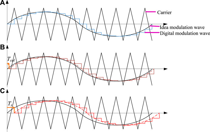
FIGURE 4. The timing sequence of the DPWM process. (A) The ideal DPWM, (B) the DPWM with the immediately updated modulation wave, (C) the DPWM with one-step delay updated modulation wave.

The calculation period is a fraction of the sample period. We assume that

$T_{cal}= \lambda T_s \left(0< \lambda <1\right)$

The z-transform can be conveniently applied to transfer the continuous system to a discrete system if T_cal is a multiple of T_s. The discrete model of the controller with this DPWM can be obtained by the modified z-transform (Mattavelli et al., 2008). The transfer function of the controlled object is defined as H(s). The discrete model of the controller can be got

$Z\left[H\left(s\right)G_{pwmb}\left(s\right)\right]=\frac{1-z^{-1}}{T_s}Z\left[\frac{H\left(s\right)}{s}{e}^{-\lambda T_{s}s}\right]=\frac{1-z^{-1}}{T_s}{Z}_m\left[\frac{H\left(s\right)}{s}\right] (3.3)$

where Z_m is the modified z-transform.

In Figure 4C, the sample begins at the peak of the triangle carrier and the digital controller produces the modulation reference. However, the modulation reference is not immediately updated until the next peak of the triangle carrier. Different from DPWM in Figures 4A,B, the additional delay of the DPWM in Figure 4C is equal to one sampling period. Thus, the transfer function of PWM is given as

$G_{pwmc}\left(s\right)=G_{dc}\left(s\right)G_{zoh}\left(s\right)=e^{-T_{s}s}\frac{1-e^{-T_{s}s}}{T_{s}s}(3.4)$

The z-transform can directly obtain the discrete model of the controller:

$Z\left[H\left(s\right)G_{pwmc}\left(s\right)\right]=\frac{1-z^{-1}}{T_{s}z}Z\left[\frac{H\left(s\right)}{s}\right](3.5)$

The delay produced by the ZOH element is inherent for the DPWM. On the contrary, the delay of the modulation update may vary with different solutions of digital control. For high-power electronic devices, a good approach implements the digital control in the DSP or the FPGA because of their high performance. In these microprocessors, the modulation signal of the PWM process and the sample of variables generally execute at the two adjacent peaks of the carrier wave. As a result, there exists the delay, T_s, for the modulation update.

In addition, the multi-sampling method is adopted in the high-power converter with low-switching-frequency in order to reduce the modulator delay (Yang et al., 2019). This method can bring the time delay, which is several times of sampling period, to the cascaded converters. As a result, the frequency-domain model of the PWM is:

$G_{pwmd}\left(s\right)=e^{-T_{d}s}\frac{1-e^{-T_{s}s}}{T_{s}s}(3.6)$

where T_d indicates different time delay and T_d maybe 0, nT_s according to the updating of the modulation reference.

Frequency-Domain Model of the Locomotive-Network System

The block diagram of the current controller is illustrated in Figure 5. Furthermore, the impedance of the traction power supply system is incorporated in the block diagram of the controller. The H_c(s) is the proportional-integral (PI) regulator of the current controller. The transfer function of the DPWM process is expressed as H_pwm(s). Different modulation update modes will lead to different H_pwm(s). Based on the analysis in “Model of the Digital Pulse Width Modulation for the Locomotive,” it can be derived by taking the time delay and the ZOH effect into consideration:

$H_{pwm}\left(s\right)=e^{-n{T}_{s}s}\frac{1-e^{-T_{s}s}}{T_{s}s}(3.7)$

The leakage inductance of the onboard transformer in the locomotive is equivalent to Z_t(s). The power supply system is equivalent as a RL circuit parallel with a capacitance. The RL branch is Z_Ls(s) and the C branch is Z_Cs(s). The parameters of Z_Ls(s) and Z_Cs(s) are related to the impedance-frequency characteristic of the traction power supply system.

FIGURE 5

FIGURE 5. The block diagram of the current controller of the VSC.

The current of the ac side (i) of the VSC is the output of the controller. The current reference (i_ref) and the voltage source (u_s) are the inputs of the controller. The output of the controller can be derived based on the multi-loop strategy in Figure 5. Thus, the transfer function is given as:

$i\left(s\right)=\frac{H_c\left(s\right)H_{pwm}\left(s\right)Y_1\left(s\right)}{1+H_c\left(s\right)H_{pwm}\left(s\right)Y_1\left(s\right)}{i}_{ref}\left(s\right)+\frac{Y_0\left(s\right)}{1+H_c\left(s\right)H_{pwm}\left(s\right)Y_1\left(s\right)}{u}_s\left(s\right)=G_{iref\to i}{i}_{ref}\left(s\right)+G_{us\to i}{u}_s\left(s\right)(3.8)$

where the Y₁(s) and Y₀(s) denote the effect of u_pwm(s) and u_s(s) on the i(s) respectively. The following two transfer functions are:

$Y_1\left(s\right)=\frac{Z_{Ls}+Z_{Cs}}{Z_t{Z}_{Ls}+Z_t{Z}_{Cs}+Z_{Ls}{Z}_{Cs}}(3.9)$

$Y_0\left(s\right)=\frac{Z_{Cs}}{Z_t{Z}_{Ls}+Z_t{Z}_{Cs}+Z_{Ls}{Z}_{Cs}}(3.10)$

The open-loop gain of the G_iref→i (s) and G_us→i (s)is:

$G_{ol}\left(s\right)=H_c\left(s\right)H_{pwm}\left(s\right)Y_1\left(s\right)(3.11)$

Therefore, the stability of the L-N system is influenced by not only the PI controller but also the DPWM dynamic and the impedance of the whole system.

The bode diagrams of the open-loop gain with the conventional PWM model and the proposed PWM model are illustrated in Figure 6. In Figure 6A, the models of the modulation updates are set as 1 in (a), the delay link of 0.5 T_s in (b), and the delay link of T_s in (c), respectively, while the dynamic of the DPWM is modeled as the same ZOH element. The magnitudes of these three different models are the same, but the phases are different. Furthermore, the gain and magnitude margin is respectively 36.8 dB/62.5° in (a), 7.6 dB/19.9° in (b), and 0.8 dB/−22.7° in (c). When these models are adopted to assess the frequency-domain stability of the system, we will obtain different results according to the gain and magnitude margins. The unstable systems may be judged as marginally stable system, which will affect the parameter design of the controller.

FIGURE 6

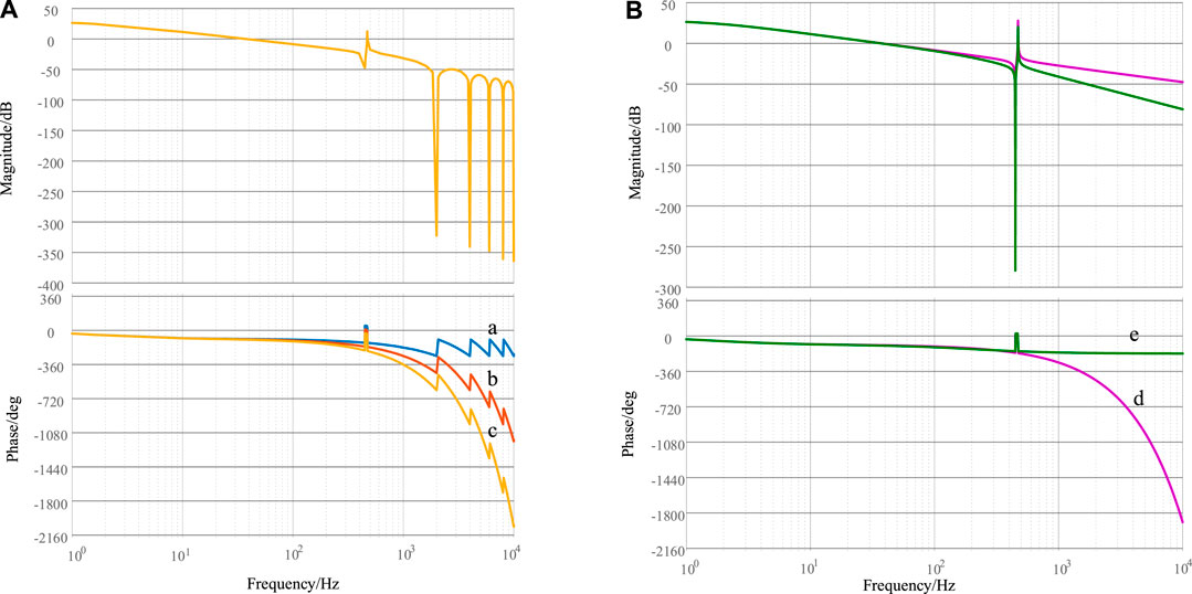
FIGURE 6. The bode diagrams of the open-loop gain (A) with different delay elements and (B) without/with DPWM dynamics: (a) only the ZOH element (b) the ZOH element and the calculation delay of 0.5 T_s (c) the ZOH element and the calculation delay of T_s (d) only the calculation delay of T_s (e) only the inertial element as the PWM model.

Afterward, the bode diagrams of the open-loop gain without the ZOH element are studied in Figure 6B. The (d) in Figure 6B displays the modeling that the modulation is updated at the next peak of the triangle carrier but the digitally discrete PWM is not taken into consideration. In addition, if the DPWM is modeled as an inertial element and the delay produced by the modulation update is ignored, the bode diagram of the open-loop gain is shown in (e) of Figure 6(B). Both the magnitude and the phase presents different frequency-domain characteristics. The phase of (e) keeps −180° for the frequency above 400 Hz. The phase margins are respectively 7.1° in (d) and 29.8° in (e). Compared with (c), the open-loop gain for (d) ignores the discrete model of the DPWM, and the positive phase margin in (d) indicates that the system is marginally stable. However, the system is assessed to be unstable because of the negative phase margin in (c). Compared with (a), the magnitude-frequency and the phase-frequency are completely different. There are four local minimums for the magnitude and the phase in (a). Thus, different frequency-domain responses will be obtained when the models are different.

Therefore, the accuracy of DPWM modeling will influence the stability assessment of the L-N system. It is necessary to include the model of the DPWM in the modeling of the whole system.

Stability Analysis and Verification

Dissipativeness of the Locomotive-Network System

To perform the stability judgment of the L-N system, the frequency-domain characteristic of the total admittance, which is also the transfer function of the voltage source to the ac current of the VSC, is analyzed. The total admittance is

$Y_{total}=G_{us\to i}= \frac{Y_0\left(s\right)}{1+H_c\left(s\right)H_{pwm}\left(s\right)Y_1\left(s\right)}(4.1)$

The K_s(s) is defined as:

$K_s\left(s\right)= \frac{Y_1\left(s\right)}{Y_0\left(s\right)}=\frac{Z_{Ls}\left(s\right)+Z_{Cs}\left(s\right)}{Z_{Cs}\left(s\right)}(4.2)$

Thus, the total admittance ${\mathit{Y}}_{\mathit{total}}\mathit{ }$can be rearranged as:

$Y_{total}= \frac{Y_0\left(s\right)}{1+H_c\left(s\right)H_{pwm}\left(s\right)K_s\left(s\right)Y_0\left(s\right)}(4.3)$

Thus, the property of the L-N system can be known as an equivalent virtual passive circuit. Based on Eq. 4.3, the block diagram of the equivalent feedback system can be given in Figure 7. In Figure 7, Y₀(s) is the forward channel and the H_c(s)H_pwm(s)K_s(s) is the feedback path.

FIGURE 7

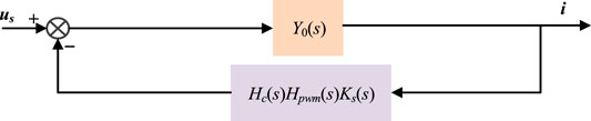
FIGURE 7. The block diagram based on the transfer function ${\mathit{G}}_{\mathit{us}\to \mathit{i}}$.

If the Nyquist curve of the open-loop gain does not encircle (−1, j0), the whole system will be stable. Then we can obtain the sufficient but not necessary condition for the system stability:

$\mathrm{Re}\left[\frac{1}{Y_0\left(j\omega \right)}\right]+\mathrm{Re}\left[H_c\left(j\omega \right)H_{pwm}\left(j\omega \right)K_s\left(j\omega \right)\right]\ge 0\mathrm{，}\text{for}\forall \omega (4.4)$

Namely,

$\mathrm{Re}\left[Z_{total}\left(j\omega \right)\right]\ge 0\mathrm{，}\text{for}\forall \omega (4.5)$

So the dissipative system is stable for all the frequencies (Harnefors et al., 2016). Namely, the positive real part of the Z_total indicates that the disturbance of the current will be dissipated and the harmonic amplification will not occur in the L-N system. However, it is difficult to ensure the system is always passive for all the frequencies. If there is a frequency region where it does not meet the requirement of Eq. 4.4, the harmonic resonance of this frequency region will be amplified because of the non-dissipative property.

The real part of Z_total(s) in equation (4-4) varying with the frequencies is displayed in Figure 8 by frequency scanning with the step of 1 Hz. The time delays are 0, T_s, 2 T_s, 3T_s, 4 T_s respectively for curve A, B, C, D, E. As shown in A, when there is no time delay, the passive region is the frequency below 1,570 Hz. Then the time delay for B is increased to T_s, and the frequency ranges of 0–1,240, 2,330–2,890 Hz are passive regions. After that, the time delay becomes to be 2 T_s for C, leading that the passive region is reduced to the frequency below 800 Hz. Then the system displays passive property below 580 Hz if the time delay is 3 T_s. The passive region is reduced for the system with the time delay 4 T_s. The frequency below 450 Hz belongs to the passive region of the system for E.

FIGURE 8

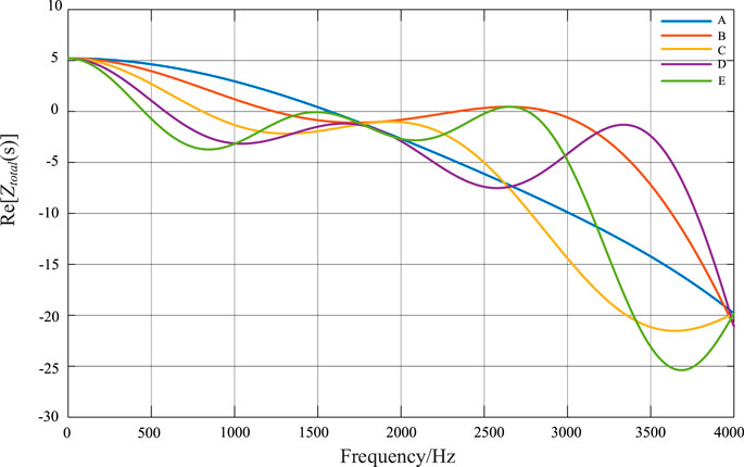
FIGURE 8. The real part of Z_total(s) with different time delays.

Consequently, the system holds the dissipative property in one frequency range while it shows the active property in other frequency ranges. In the same frequency region, the systems with different time delays may present opposite properties. The disturbance in the frequency range of the non-dissipative region will excite the instability phenomenon.

Time-Domain Simulation Results

To validate the frequency-domain analysis based on the dissipative property which is influenced by the digital time delay of the DPWM, the L-N system in Figure 3 is established in the discrete time-domain models by using the simulation software Matlab/Simulink. Table 1 lists five cases which are corresponding to five kinds of DPWM time delays. The frequency change of the inherent harmonic resonance is carried out by changing the length of the traction network.

TABLE 1

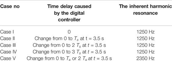
TABLE 1. Five simulated cases corresponding to four kinds of time delays.

The modeling of the traction power supply system is briefly described in this section. The traction power supply system consists of the traction substation and the traction network. The main part of the traction substation is the traction transformer whose inductance parameter is important to the impedance-frequency characteristics of the traction power supply system. The traction network is modeled as a multi-conductor transmission lines because of its distributed parameters. As shown in Figure 9, the equivalent π-circuit of a transmission line is adopted to model the conductors of the traction network. In Figure 9, the equivalent π-circuit can be calculated by

$\begin{array}{l}\{\begin{array}{c}{Z}_L=\sinh \left(\sqrt{ZY}l\right){\left(ZY\right)}^{-\frac{1}{2}}\\ \frac{Y_L}{2}=Y{\left(ZY\right)}^{-\frac{1}{2}}\tanh \left(\frac{\sqrt{ZY}l}{2}\right)\end{array}\\ \end{array}(4.6)$

where Z, Y, and l are respectively the impedance parameter matrix, the admittance matrix, and the length of the line (Mingli et al., 2010). Based on the equivalent π-circuit of a transmission line in Eq. (4.6), the entire traction network can be modeled as an equivalent 6-conductor line consisting of uplink and downlink contact lines (T1, T2), rails (R1, R2) and feeders (F1, F2). The entire feeding section can be cut into several units by the shunt or series elements. The 6-conductor line model of the traction network is visualized in Figure A1. The parameters of the self-inductance, the mutual-inductance, the self-capacitance, and the mutual-capacitance are list in Table A1. Moreover, the parameters of the traction substation are list in Table 2.

FIGURE 9

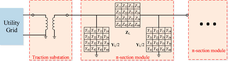
FIGURE 9. The π-section module of the traction network.

TABLE 2

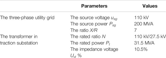
TABLE 2. The simulation parameters of the substation.

The VSC simulation model of the locomotive composites the power electronic circuit and its discrete controller. The function-call subsystem block of Simulink implements the discrete controller. The function-call subsystem is executed by the interrupt trigger signal whose period is the same as the sampling period. It connects with the traction power supply system through the PCC. The parameters of the converter are presented in Table 3.

TABLE 3

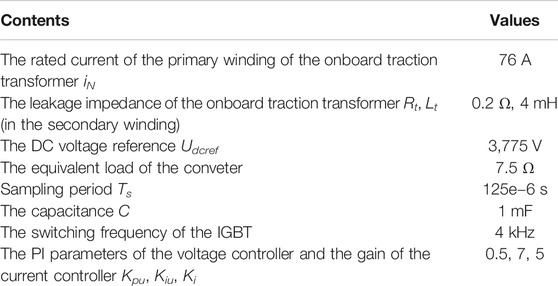
TABLE 3. The simulation parameters of the converters.

The time delay is carried out after the L-N system runs stably. The controller does not work until the two pre-charging processes are finished at t = 1.2 s. Then the controller starts to work and the DC voltage reference ramps up to 3,775 V. The DC voltage can arrive at 3,775 V at t = 1.5 s. At t = 2 s, the load of the converter is on. At t = 3.5 s, the time delay in case I–V is added in the discrete controller of the converter.

Figure 10 shows the simulated voltage and the simulated voltage waveforms of the PCC for case I. The stable response can be observed in (A). There is no amplified harmonic resonance because the real part of the impedance is positive. The spectra of the voltage are displayed in Figure 10 (B). The harmonic content of the voltage for the 1250 Hz is 2.86% at t = 3.52 s, which is higher than other harmonics. The simulation result responds to the dissipative property of the system in the frequency range from 0 to 1250 Hz in Figure 10C.

FIGURE 10

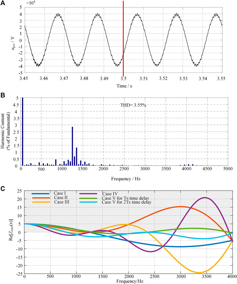
FIGURE 10. The simulated waveforms and the harmonic spectra for case I (A) voltage of the PCC, (B) harmonic spectra of u_PCC, (C) the real part of Case I ∼ V.

The simulated waveforms for case II are illustrated in Figure 11. The time delay T_s is added at t = 3.5 s. It shows that the simulated voltage maintains stable although there is a time delay of T_s for the modulation. As displayed in Figure 10C, the real part of the Z_total is positive for the whole frequency range so that the non-dissipative property is not so powerful. As a result, the inherent harmonic resonance is not amplified when the time delay is increased to T_s. The THD of u_pcc is 3.53% at t = 3.4 s and 2.39% at t = 3.52 s. The harmonic characteristics are not deteriorated despite the T_s time delay. Then, the simulation result of u_pcc for case III is depicted in Figure 12. From 3.5 s, the 2 T_s time delay is set in the controller. Although the minimum of the real part is -0.69Ω for the frequency range of 800Hz∼1250Hz in Figure 10C, there is no apparent harmonic amplification quickly after the time delay. It should be noted that it is difficult to obtain the totally accurate theoretical model because of the complexity of the actual system.

FIGURE 11

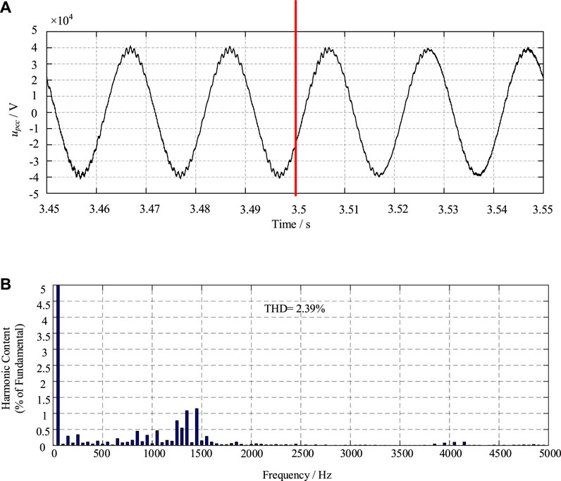
FIGURE 11. The simulated waveforms and the harmonic spectra for case II (A) voltage of the PCC, (B) harmonic spectra of u_PCC.

FIGURE 12

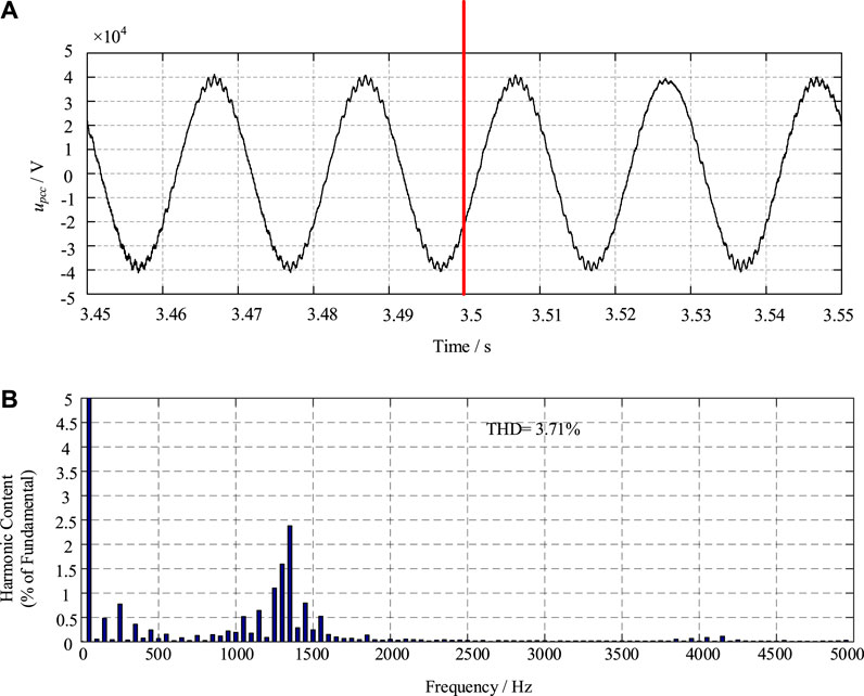
FIGURE 12. The simulated waveforms and the harmonic spectra for case III (A) voltage of the PCC, (B) harmonic spectra of u_PCC.

Moreover, Figure 13 illustrates the waveforms of u_pcc for case IV. The system comes into the unstable condition quickly. The amplitude of the voltage is amplified seriously after 3.5 s. Consequently, the L-N system cannot operate normally and the overvoltage will occur in the traction network because of the amplified harmonic resonance. The frequency of the passive region is below 580 Hz, and the minimum of the real part is -1.85Ω for the frequency range of 575Hz∼1250Hz in Figure 10C. The high negative resistance gives rise to the occurrence of the harmonic resonance amplification.

FIGURE 13

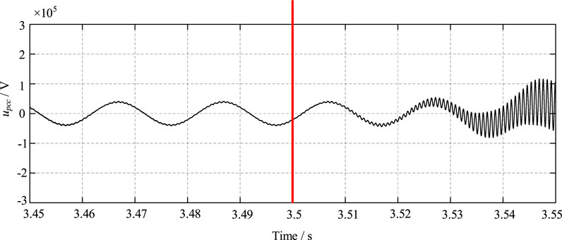
FIGURE 13. The simulated waveforms of voltage of the PCC for case IV.

Specifically, case V is carried out to investigate the influence of the traction power supply system on the real part of the total impedance. The inherent resonance frequency is the frequency of the impedance magnitude peak. The impedance relates to the length of the traction network (Holtz and Kelin, 1989). So the impedance change of the traction power supply system can be carried out through reducing the length of the traction network. The inherent resonance frequency is 2,350 Hz in case V. The simulated result is given in Figures 14. The real part of the Z_total at 2,350 Hz belongs to the non-dissipative region to the system with 2 T_s time delay. Because of this passive property, the harmonic resonance is amplified quickly for the simulated waveform of u_pcc after 3.5 s for 2 T_s time delay as shown in Figure 14B. However, the L-N system keeps stable in Figure 14A. It indicates that the increase in the time delay leads to harmonic amplification. Nevertheless, the frequency depends on the inherent frequency of the traction network.

FIGURE 14

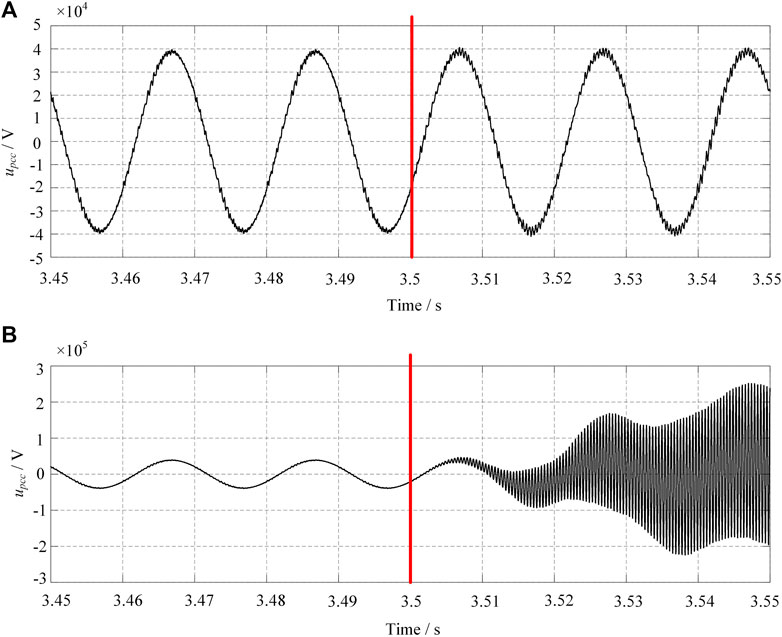
FIGURE 14. Simulation result for case V. (A) the simulated voltage waveform for T_s time delay (B) the simulated voltage waveform for 2 Ts time delay.

Based on the investigation mentioned above, the simulation results of these five cases corresponds to the theoretical analysis based on the dissipative of the L-N system. In case I, when there is no time delay for the modulation, the L-N system can maintain stable. In case II, where the T_s time delay is added, the stability of the L-N system is not deteriorated severely because of its passive property. Different from the simulation result of case III, the harmonic resonance of 1,250 Hz in case IV is quickly amplified seriously because of its deeply negative real part of the total impedance. Moreover, case V is conducted in order to validate the influence of the main circuit of the traction network on the dissipative L-N system. The harmonic amplification of 2,350 Hz occurs quickly for case V with 2 T_s. Therefore, the time delay margin varies with different systems.

Experiment Results

The time-domain experiment is conducted in the laboratory environment utilizing the hardware-in-loop (HIL) test bench to validate the presented analysis and simulation. The controller of the VSC is implemented in the DS1007 board of the dSPACE system through the discretization of the regulator. The main circuit of the VSC is established based on a single-phase H-bridge, a pre-charge circuit and a grid simulator. The grid simulator is adopted to simulate the power source. The pre-charge circuit is switched by the digital signals to charge the capacitor of the DC side. For the power supply system, the practical approach of the experiment in the laboratory is to adopt an RLC circuit. The parameters are listed in Table 4. The load of the converter is a resistor which is in parallel with the DC capacitance.

TABLE 4

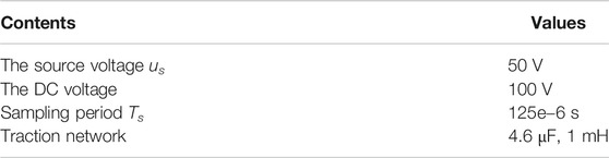
TABLE 4. The parameters of the down-scale platform.

Four groups of experiments are carried out based on the simulation cases. As shown in Figure 15A, when there is no load for the DC side of the converter, the harmonic content of the AC side current is much high. The experiment result of the converter with load is displayed in Figure 15B. There is a ripple for the DC voltage, and the AC side current is sinusoidal. Then in Figure 15C, the time delay of T_s is set in the discrete controller. The system is still stable, but there is a phase difference between the current and the voltage. In Figure 15D, the time delay of 2 T_s is added to a stable system. As shown in Figure 15B, the L-N system is not stable so that the relay protection is triggered. The system is switched off. So the harmonic amplification is not observed in the experiment result.

FIGURE 15

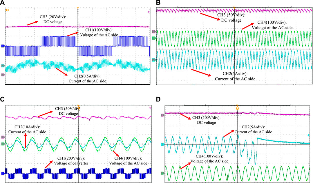
FIGURE 15. The HIL experiment result of (A) zero time delay for the converter without load, (B) zero time delay for the converter with load, (C)T_s time delay, (D) 2 T_s time delay.

Conclusion

The frequency-domain impedance of the L-N system is derived by taking the control delay and the ZOH effect of the DPWM into consideration. Then the stability of the L-N system is assessed by the passive property of the total impedance. The inherent harmonic resonance will be amplified if the inherent resonance frequency locates in the non-dissipative region of the L-N system. Furthermore, the impedance of the traction network influences the dissipative property of the L-N system. By the comparison of case I-IV, the harmonic resonance amplification of 1,250 Hz occurs when the 3 T_s time delay is set in the converter controller. In case V, the harmonic resonance amplification of 2,350 Hz occurs when the 2 T_s time delay is added. Furthermore, before a new electric railway or a new type of locomotive is put into use, the harmonic resonance can be predicted to avoid the occurrence of the instability phenomenon and the damage of the electrical equipment.

Data Availability Statement

All datasets generated for this study are included in the manuscript/supplementary files.

Author Contributions

JL: methodology; JL, YZ, and QL: modeling of the power supply system; JL and QL: modeling of the locomotive and experiment validation; MW and MM: supervision.

Funding

This work was supported by the Fundamental Research Funds for the Central Universities under Grant 2018JBZ101 and China Postdoctoral Science Foundation under Grant 2020M670124.

Conflict of Interest

The authors declare that the research was conducted in the absence of any commercial or financial relationships that could be construed as a potential conflict of interest.

Appendix

FIGURE A1

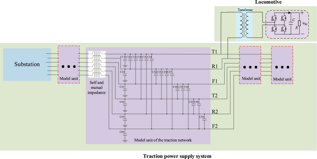
FIGURE A1. The illustration of the L-N system simulation model.

TABLE A1

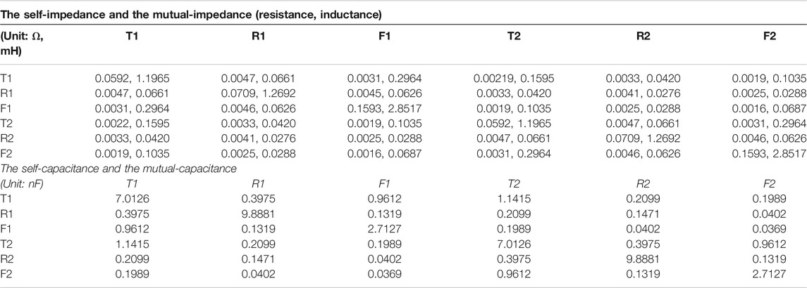
TABLE A1. The parameters of the 6-conductor lines simulation model.

References

Amin, M., and Molinas, M. (2017). Small-signal stability assessment of power electronics based power systems: a discussion of impedance- and eigenvalue-based methods. IEEE Trans. Ind. Appl. 53 (5), 5014–5030. doi:10.1109/tia.2017.2712692 CrossRef Full Text

Google Scholar

Buso, S., and Mattavelli, P. (2006). Digital control in power electronics. San Rafael, CA: Morgan & Claypool.

Google Scholar

Cui, H., Feng, X., Ge, X., Fang, H., and Song, W. (2015). Resonant harmonic elimination pulse width modulation-based high-frequency resonance suppression of high-speed railways. IET Power Electron. 8 (5), 735–742. doi:10.1049/iet-pel.2014.0204 CrossRef Full Text

Google Scholar

de Castro, A., Zumel, P., Garcia, O., Riesgo, T., and Uceda, J. (2003). Concurrent and simple digital controller of an AC/DC converter with power factor correction based on an FPGA. IEEE Trans. Power Electron. 18 (1), 334–343. doi:10.1109/tpel.2002.807106

CrossRef Full Text | Google Scholar

Dorf, R. C., and Bishop, R. H. (2016). Modern control systems. 13th Ed. Hoboken, NJ: Pearson Education.

Google Scholar

Harnefors, L., Zhang, L., and Bongiorno, M. (2008). Frequency-domain passivity-based current controller design. IET Pwr. Electr. 1 (4), 455. doi:10.1049/iet-pel:20070286 CrossRef Full Text

Google Scholar

Harnefors, L., Bongiorno, M., and Lundberg, S. (2007). Input-admittance calculation and shaping for controlled voltage-source converters. IEEE Trans. Ind. Electron. 54 (6), 3323–3334. doi:10.1109/tie.2007.904022 CrossRef Full Text

Google Scholar

Harnefors, L., Wang, X., Yepes, A. G., and Blaabjerg, F. (2016). Passivity-based stability assessment of grid-connected VSCs—an overview. IEEE J. Emerg. Sel. Topics Power Electron. 4 (1), 116–125. doi:10.1109/jestpe.2015.2490549 CrossRef Full Text

Google Scholar

Holtz, J., and Kelin, H.-J. (1989). The propagation of harmonic currents generated by inverter-fed locomotives in the distributed overhead supply system. IEEE Trans. Power Electron. 4 (2), 168–174. doi:10.1109/63.24900 CrossRef Full Text

Google Scholar

Kolar, V., Palecek, J., Kocman, S., Trung Vo, T., Orsag, P., Styskala, V., et al. (2010). “Interference between electric traction supply network and distribution power network—resonance phenomenon,” in Proceedings of 14th international conference on harmonics and quality of power - ICHQP, Bergamo, Italy, September 26--29, 2010 (Piscataway, NJ: IEEE). 1–4.

Google Scholar

Kostic, D. J., Avramovic, Z. Z., and Ciric, N. T. (2013). A new approach to theoretical analysis of harmonic content of PWM waveforms of single- and multiple-frequency modulators. IEEE Trans. Power Electron. 28 (10), 4557–4567. doi:10.1109/tpel.2012.2232309 CrossRef Full Text

Google Scholar

Lee, H., Lee, C., Jang, G., and Kwon, S. (2006). Harmonic analysis of the Korean high-speed railway using the eight-port representation model. IEEE Trans. Power Deliv. 21 (2), 979–986. doi:10.1109/tpwrd.2006.870985 CrossRef Full Text

Google Scholar

Li, J., Wu, M., Molinas, M., Song, K., and Liu, Q. (2019). Assessing high-order harmonic resonance in locomotive-network based on the impedance method. IEEE Access 7, 68119–68131. doi:10.1109/access.2019.2918232 CrossRef Full Text

Google Scholar

Liu, Z., Zhang, G., and Liao, Y. (2016). Stability research of high-speed railway EMUs and traction network cascade system considering impedance matching. IEEE Trans. Ind. Appl. 52 (5), 4315–4326. doi:10.1109/tia.2016.2574770 CrossRef Full Text

Google Scholar

Mattavelli, P., Polo, F., Dal Lago, F., and Saggini, S. (2008). Analysis of control-delay reduction for the improvement of UPS voltage-loop bandwidth. IEEE Trans. Ind. Electron. 55 (8), 2903–2911. doi:10.1109/tie.2008.918607 CrossRef Full Text

Google Scholar

Mingli, W., Roberts, C., and Hillmansen, S. (2010). “Modelling of AC feeding systems of electric railways based on a uniform multi-conductor chain circuit topology,” in IET conference on railway traction systems (RTS), Birmingham, UK, April 13-15, 2010. Stevenage: IET.

Google Scholar

Mouton, H. d. T., McGrath, B., Holmes, D. G., and Wilkinson, R. H. (2014). One-dimensional spectral analysis of complex PWM waveforms using superposition. IEEE Trans. Power Electron. 29 (12), 6762–6778. doi:10.1109/tpel.2014.2304677 CrossRef Full Text

Google Scholar

Nguyen, C., Duong, T., Duong, M., and Le, D. (2020). Chattering-free single-phase robustness sliding mode controller for mismatched uncertain interconnected systems with unknown time-varying delays. Energies 13 (1), 1383–1396. doi:10.3390/en13010282 CrossRef Full Text

Google Scholar

Paice, A. D. B., and Meyer, M. (2000). “Rail network modelling and stability: the input admittance criterion,” in 14th International Symposium on mathematical theory Network System, June 19-23, 2020, France: Perpignan.

Google Scholar

Qiujiang, L., Mingli, W., Junqi, Z., Kejian, S., and Liran, W. (2018). Resonant frequency identification based on harmonic injection measuring method for traction power supply systems. IET Power Electron. 11 (3), 585–592. doi:10.1049/iet-pel.2017.0122 CrossRef Full Text

Google Scholar

Rygg, A., Molinas, M., Zhang, C., and Cai, X. (2016). A modified sequence-domain impedance definition and its equivalence to the dq-domain impedance definition for the stability analysis of AC power electronic systems. IEEE J. Emerg. Sel. Topics Power Electron. 4 (4), 1383–1396. doi:10.1109/jestpe.2016.2588733 CrossRef Full Text

Google Scholar

Sainz, L., Cheah-Mane, M., Monjo, L., Liang, J., and Gomis-Bellmunt, O. (2017). Positive-net-damping stability criterion in grid-connected VSC systems. IEEE J. Emerg. Sel. Topics Power Electron. 5 (4), 1499–1512. doi:10.1109/jestpe.2017.2707533 CrossRef Full Text

Google Scholar

Song, K., Mingli, W., Yang, S., Liu, Q., Agelidis, V. G., and Konstantinou, G. (2019). High-order harmonic resonances in traction power supplies: a review based on railway operational data, measurements and experience. IEEE Trans. Power Electron. 35 (3), 2501–2518. doi:10.1109/tpel.2019.2928636

CrossRef Full Text | Google Scholar

Song, K., Konstantinou, G., Mingli, W., Acuna, P., Aguilera, R. P., and Agelidis, V. G. (2017). Windowed SHE-PWM of interleaved four-quadrant converters for resonance suppression in traction power supply systems. IEEE Trans. Power Electron. 32 (10), 7870–7881. doi:10.1109/tpel.2016.2636882 CrossRef Full Text

Google Scholar

Song, W., Jiao, S., Li, Y. W., Wang, J., and Huang, J. (2016). High-frequency harmonic resonance suppression in high-speed railway through single-phase traction converter with LCL filter. IEEE Trans. Transp. Electrific. 2 (3), 347–356. doi:10.1109/tte.2016.2584921 CrossRef Full Text

Google Scholar

Tan, P.-C., Loh, P. C., and Holmes, D. G. (2005). Optimal impedance termination of 25-kV electrified railway systems for improved power quality. IEEE Trans. Power Deliv. 20 (2), 1703–1710. doi:10.1109/tpwrd.2004.834308 CrossRef Full Text

Google Scholar

Wang, X., Harnefors, L., and Blaabjerg, F. (2018). Unified impedance model of grid-connected voltage-source converters. IEEE Trans. Power Electron. 33 (2), 1775–1787. doi:10.1109/tpel.2017.2684906 CrossRef Full Text

Google Scholar

Wu, L., and Mingli, W. (2017). Single-phase cascaded H-bridge multi-level active power filter based on direct current control in AC electric railway application. IET Power Electron. 10 (6), 637–645. doi:10.1049/iet-pel.2016.0760 CrossRef Full Text

Google Scholar

Yang, J., Liu, J., Shi, Y., Zhao, N., Zhang, J., Fu, L., et al. (2019). Carrier-based digital PWM and multirate technique of a cascaded H-bridge converter for power electronic traction transformers. IEEE J. Emerg. Sel. Topics Power Electron. 7 (2), 1207–1223. doi:10.1109/jestpe.2019.2891735 CrossRef Full Text

Google Scholar

Zhang, C., Molinas, M., Rygg, A., Lyu, J., and Cai, A. (2019a). Harmonic transfer function-based impedance modelling of a three-phase VSC for asymmetric AC grids stability analysis. IEEE Trans. Power Electron. 34 (12), 12552–12566. doi:10.1109/tpel.2019.2909576

CrossRef Full Text | Google Scholar

Zhang, C., Molinas, M., Rygg, A., and Cai, A. (2019b). Impedance-based analysis of interconnected power electronics systems: impedance network modeling and comparative studies of stability criteria. IEEE J. Emerg. Selected Topics Power Electron. 8 (3), 2520–2533. doi:10.1109/jestpe.2019.2914560

CrossRef Full Text | Google Scholar

Zhang, R., Liu, S., Lin, F., Cao, H., Liu, Y., and Han, K (2017). “Resonance influence factors analysis of high-speed railway traction power supply system based on RT-LAB,” in 2017 IEEE transportation electrification conference and expo, August 7–10, 2017, Harbi, China (IEEE).

Google Scholar