Modeling the Effects of Agricultural Innovation and Biocapacity on Carbon Dioxide Emissions in an Agrarian-Based Economy: Evidence From the Dynamic ARDL Simulations

In this paper, we modeled the effects of income, agricultural innovation, energy utilization, and biocapacity on Carbon dioxide (CO₂) emissions. We tested the validity of the environmental Kuznets curve (EKC) hypothesis for Nigeria from 1981 to 2014. We applied the novel dynamic autoregressive distributed lag (ARDL) simulations to develop conceptual tools for policy formulation. The empirical results confirmed the EKC hypothesis and found that agricultural innovation and energy utilization have an escalation effect on CO₂ emissions whereas income and biocapacity have long-run emission-reduction effects. The causality results found agricultural innovation attributable to CO₂ emissions and observed that income drives energy demand. Income, biocapacity, and energy utilization are found to predict changes in CO₂ emissions. These results are validated by the innovation accounting techniques—wherein 22.79% of agricultural innovation corresponds to 49.43% CO₂ emissions—5.95% of biocapacity has 35.78% attributable CO₂ emissions—and 1.61% of energy spurs CO₂ emissions by 16.27%. The policy implication for this study is that energy efficiency, clean energy utilization and sustainable ecosystem recovery and management are the surest ways to combat climate change and its impacts.

Introduction

Mitigation of climate change and its impacts on the environment and wellbeing are important global issues in recent times. Climate change has a traceable course to excessive use of “unclean” combustible energy, which disrupts the levels of carbon in the atmosphere, resulting to the preservation of heat in the atmosphere (See Kasman and Duman, 2015; Usman et al., 2019; Rafindadi and Usman, 2019; Agboola and Bekun, 2019; Usman et al., 2020a; Usman et al., 2020b). Research on energy utilization and economic outgrowth effects of CO₂ emissions has received significant attention in the literature of environmental management. Essentially, within the theoretical account of Environmental Kuznets Curve (EKC) hypothesis, it is reported that economic development initially triggers environmental pollution with increasing levels of income but declines afterward at specified threshold of income level where environmental awareness remains a priority (Grossman and Krueger, 1991).

A significant number of the extant literature have tested the validity of the EKC hypothesis over the years lacking consensus. The empirical results from most studies are that economic growth trajectory heightens environmental pollution but declines thereafter following improvements in livelihood and environmental awareness, thereby validating the EKC hypothesis (Shahbaz et al., 2013; Rafindadi, 2016; Shahbaz et al., 2017; Mesagan et al., 2018; Rafindadi and Usman, 2019). On the contrary, some studies aptly posit that energy-intensive economic outgrowth and environmental quality is not in line with the EKC hypothesis (Inglesi-Lots and Bohlmaann 2014; Nasr et al., 2015). Therefore, the EKC-based empirical findings are mixed and conflicting, hence, require further empirical validation. Despite mitigating efforts by world leaders geared toward CO₂ sequestration, a substantial rising of the contribution of CO₂ to greenhouse gas (GHG) emissions are reported over the years (IPCC, 2017). It is reported that CO₂ contributes 76.6% of GHG emissions generated mostly by developing economies in the quest to sustain economic productivity. Between 1961 and 2011, CO₂ emissions rose from ∼9.4 billion metric tons to ∼34.6 billion metric tons (IPCC, 2013). Equally, CO₂ emissions increased from ∼29.7 billion tons to ∼33.4 billion tons between 1999 and 2017 (BP, 2018). In Nigeria, CO₂ emissions remain a major threat to both human and ecosystem development. As reported by the World Bank (2015), as of 2014, Nigeria emitted 96,280.75 kilotons of CO₂, which was lower than 106,067.98 kilotons in 2005.

A large body of literature has linked climate change to agricultural practices. As recently emphasized by Owusu and Asumadu (2016), Shabbir et al. (2020), Agboola and Bekun (2019), in addition to excessive consumption of energy from the fossil fuel sources, agricultural practices have a substantial effect on GHG emissions. Agriculture ranked is as the second-highest contributor of GHG emissions and global warming, contributing roughly 21% of the global anthropogenic GHG emissions in the world (Blanco et al., 2014). This is because most agricultural practices require greater energy consumption, mostly sourced from fossil fuels (Blanco et al., 2014). Agriculture may affect the ability of land to absorb heat and light, which can lead to radioactive forcing. More so, deforestation and desertification resulting from land use and fossil fuels can exert upward pressure on anthropogenic carbon dioxide. Besides, raising livestock such as cattle, pigs and poultry may contribute to methane and nitrous oxide concentrations and emissions. On the other hand, agriculture can substantially reduce the level of carbon emissions as opined by the United Nations Food and Agricultural Organization (FAO), (2016). This is supported by Reynolds and Wenzlau (2012) who posit that agriculture innovation is reported to have a mitigation effect on CO₂ emissions. For example, some modern agricultural practices can be powered by clean energy to reduce the effects of the use of pesticides, irrigation, soil tillage, deforestation, and waste from the plastic mulch, stubble burning, and other channels of GHG emissions.

Our study, therefore, hypothesizes that the effects of agricultural innovation and biocapacity on CO₂ emissions have long- and short-term environmental consequences in Nigeria. Given that Nigeria is an agrarian nation blessed with natural resources, there are reports of its citizens engaging in crude methods of agricultural practices that hamper environmental sustainability. However, scientific literature on the scope is limited for policy formulation. More so, Nigeria is ranked among the top 10 countries with a dangerous precedent of ambient air pollution (HEI, 2018). Besides, a recent study ranked Nigeria as the sixth among 195 nations with the most approximate cases of disability-adjusted life years from exposure to air pollution (Owusu and Sarkodie, 2020a). Thus, justifies the need to investigate the effects of agricultural innovation and ecosystem dynamics on CO₂ emissions. This will have policy implication not only on carbon sequestration but mitigating mortality and morbidity rates. Therefore, insights from our study will provide supporting evidence for policymakers in designing appropriate energy and environmental policies for CO₂ sequestration that underpins the Sustainable Development Goals (SDGs). In terms of methodology, we use Lee-Strazicich (L-S) structural break, causality test and novel dynamic autoregressive distributed lag (ARDL) simulations approach—to estimate the out-sample parameters of counterfactual shocks in specific time periods and specified exogenous regressor useful for policy formulation. This is the first time such a novel out-sample, stochastic and simulation technique has been utilized in extant literature for the proposed theme.

Literature Review

The EKC hypothesis from the pioneering work of Kuznets (1955) underpins the framework for this study. In its generic form, Kuznets observed a nexus between income per capita and inequality in such that income inequality would first rise and decline as income increases. This hypothesis led to what is known as EKC by Grossmann and Krueger (1991). The EKC hypothesis postulates a parallel increase of both income level and emissions until a threshold of income is achieved before a reduction in emissions can be noticed thereafter. This hypothesis explains the trade-off between sustained economic productivity and environmental sustainability.

The nexus between economic productivity and ecological degradation has gained prominence in extant literature since the mid-90s. For example, a study found an “inversed U-shaped” relationship where ecological pollution would increase at the early stages of economic development but after a specified threshold, economic outgrowth tends to mitigate ecological pollution (Selden and Song, 1994). Similarly, several studies have all reported an inverted U-shaped nexus between economic growth and CO₂ emissions (Galeotti et al., 2006; Shahbaz et al., 2013; Rafindadi and Usman, 2019; Ike et al., 2020a; Usman et al., 2020b). For example, Shahbaz et al. (2013) applied the ARDL cointegration approach to investigate the effect of energy intensity, economic growth, and globalization on CO₂ emissions in Turkey. The findings documented the presence of EKC and further revealed economic growth and energy intensity exert positive pressure on CO₂ emissions while globalization reduces CO₂ emissions. Similarly, a study by Rafindadi and Usman (2019) using ARDL modeling approach with controlled structural breaks validated the EKC hypothesis for South Africa. A recent paper by Ike et al. (2020a) using a novel quantile regression via quantile moments confirmed the EKC hypothesis by controlling for oil production in oil producing nations.

On the contrary, some studies reported that the EKC hypothesis might not hold always. For example, “N-shaped” relationship between productivity and emissions following a hike in CO₂ emission was observed for a small open economy and industrialized country (Fried and Getzner, 2003). Similarly, it is reported that the validity of the EKC is not certain in all circumstances, hence, there is no certainty that an inversed-U shaped link exists between economic productivity and pollution (See Spangenberg, 2001). In a study by Nasr et al. (2015) found no evidence to support the EKC in South Africa using a co-summability technique with a century of data.

In recent times, many studies have incorporated the role of energy utilization in testing the validity of the conventional EKC hypothesis. The EKC hypothesis was tested in Romania by incorporating energy utilization (Shahbaz et al., 2013). The findings confirmed the EKC hypothesis and further revealed energy utilization attributable CO₂ emissions. Tiwari et al. (2013) found EKC and bi-directional causality between growth and CO₂ emissions from accounting for coal, growth, and trade in India. This means that economic growth first increases with environmental pollution but after reaching a turning point, increasing productivity improves environmental quality. Using the ARDL approach for Portuguese economy over the period 1971 to 2008, the EKC was validated in both short- and long-run in the presence of international trade, urbanization, and energy consumption. The effects of coal energy, industrial production and emissions were investigated in China and India (Shahbaz et al., 2014). The results identified an inversed U-shaped for India and U-shaped for China. It further showed that coal consumption causes CO₂ emissions in India while the feedback effect is observed in China. The impact of energy and democracy on CO₂ emissions was investigated in India using the ARDL methodology and found that, while energy increases CO₂ emissions, democracy perhaps mitigates emissions (Usman et al., 2019). Also, Usman et al. (2020b) incorporated globalization, democracy, and energy consumption in a standard EKC model for South Africa and confirmed an inversed U-shaped link between growth and emissions of CO₂. Similarly, the EKC hypothesis was confirmed in Thailand, using heterogeneous fossil fuel sources (Ike et al., 2020a).

Based on panel data settings, the interaction of income and CO₂ emissions was assessed in 43 developing countries (Narayan and Narayan, 2010). The results revealed that CO₂ emissions significantly dropped with a rise in income, suggesting that the hypothesis of EKC fails to hold. Conversely, Apergis (2016) investigated the real GDP-CO₂ emissions nexus in 15 countries and showed evidence of the EKC in most of the countries. More recently, Ike et al. (2020b) reported EKC for 15 oil-producing countries while exogenizing crude oil, electricity, trade, and democracy. This understanding is supported by Ike et al. (2020c) who found EKC for a panel of G-7 both in country-specific and panel settings.

Unlike most studies, very few pieces of extant literature tested for the EKC by exogenizing agricultural production. For example, evidence of EKC with agriculture reducing the level of CO₂ emissions in Turkey was reported (Dogan, 2016). Gagnon et al. (2016) divulged that agriculture has no impact significantly on emissions of carbon dioxide in Canada. Gokmenoglu and Taspinar (2018) investigated the role of agriculture in inducing CO₂ emissions in Pakistan. The empirical results observed the existence of EKC and further discovered that agriculture increases CO₂ emissions. Furthermore, feedback causal relationships are noticed among GDP, energy, agriculture, and CO₂ emissions. The EKC position in Nigeria examined by controlling for agriculture and foreign direct investment (Agboola and Bekun, 2019). The results obtained echoed the EKC hypothesis and thus documented that agriculture deteriorates the environment in Nigeria.

A panel data methodology was used to analyze the effect of agriculture on CO₂ emissions for Southeast Asian countries (Liu et al., 2017). The finding failed to lend support for the EKC. The study revealed that agriculture reduces CO₂ emissions with causality from renewables to CO₂ emissions and from growth to agriculture. On the contrary, an increase in agriculture was found to reduce CO₂ emission in five MENA countries (Ben Jebli and Ben Youssef, 2017). Based on the causality, it was discovered that agriculture Granger-cause economic growth while energy causes agriculture. However, the bi-directional linkage was found for agriculture and CO₂ emissions. These findings of course are similar to Olanipekun et al. (2019) who found a positive effect of agricultural production on pollution in Africa.

The existing literature on agriculture-induced CO₂ emissions is very few and scanty, particularly for Nigeria. The only existing country-specific study on Agriculture-CO₂ emission linkage in Nigeria is a recent study by Agboola and Bekun (2019), which suffers from misspecification problems. For example, the authors used the log forms of agricultural value-added and trade which are in percentages and hence growth rates. Taking a log of growth rate is technically wrong and could lead to spurious regression. Another methodology problem suffered by the study is the application of a standard Granger causality test withoutf meeting its fundamental assumption. As noted in the literature, a traditional Granger causality is used only when the series are all in levels. The work by Olanipekun et al. (2019) is based on the panel of African countries, which have country-specific problems. Therefore, the findings may have limited policy implications for Nigeria. Also, the existing studies failed to capture structural breaks in the variables which could alter CO₂ emissions in the long run. Therefore, to properly model agriculture-induced CO₂ emissions and EKC in Nigeria, we incorporated the structural breaks into our model to examine their effects on the endogenous variable in the long run. Finally, since Nigeria is blessed with diverse natural resources, we control for biocapacity to capture the ability of the ecosystem to produce biological materials demand of the people.

Materials and Methods

Data Collection

We employed time-series data spanning 1981–2014, selected due to data availability.¹ The variables in the models include CO₂ emissions per capita as an endogenous variable while real GDP per capita, which represents “second order polynomial of real GDP per capita (GDP²), agricultural value-added; biocapacity and energy per capita (EU) are exogenous variables. Generally, CO₂ emission per capita measures environmental quality. Real GDP per capita is used as a proxy for income or wealth, agricultural value-added per capita is used as a proxy for agricultural innovation since value is added to the raw materials of agriculture while Biocapacity per capital measures the ecosystem recovery. CO₂ emissions, real GDP, agricultural innovation measured by agricultural value-added, and Energy Use are obtained from the World Development Indicators (WDI) database,² while Biocapacity is retrieved from the Global Footprint Network (GFN) database.³⁴

The selections of these variables are guided by the United Nations’ long-term plan for Sustainable Development Goals (SDGs) which emphasizes clean energy, growth, and environment. Particularly, we included energy use to tackle goal 6, which targets clean energy and water, energy use. Goal 7, which is centered on the affordability of clean energy, is facilitated by improvement in agriculture and biocapacity. We believe that once agriculture is stimulated coupled with biocapacity, people would be able to afford clean energy. We included GDP to capture goal 8, which is concerned with achieving decent work and growth without causing damage to the environment. Finally, goals 9 and 13, which are concerned with climate change and carbon sequestration, are represented by CO₂ emissions. The variables, measurements and source are described in Table 1.

TABLE 1

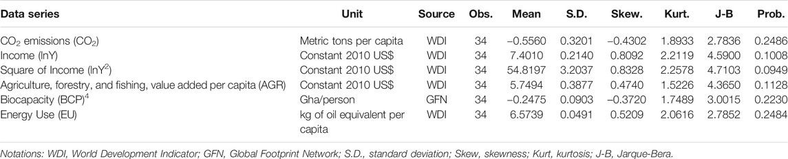
TABLE 1. Features of data series using descriptive statistics.

Model Specification

Following Shahbaz et al. (2013), Mesagan et al. (2018), Rafindadi and Usman (2019), Usman et al. (2020b), the standard EKC framework is expressed as:

$C{O}_{2t}={\Phi }_0+{\alpha }_1{Y}_t+{\alpha }_2{Y}_t^2+{\mu }_t(1)$

Where ${\Phi }_0$ is the constant, ${\text{CO}}_2$ is the carbon emissions, which measure environmental quality. $Y_t$ is Real GDP, which measures income while the squared term of real GDP $\left(Y_t^2\right)$ is added to determine whether the validity of the EKC hypothesis. ${\mu }_t$ embodies the error term that is invariably presumed to be normally distributed. In this study, we incorporated agricultural and biocapacity variables into the standard EKC framework. This is because, agricultural activities and biocapacity of a country could contribute or mitigate the rate of carbon emissions as documented in the earlier studies by Dogan (2016), Sarkodie et al. (2019). Therefore, our model will be expressed as follows:

$C{O}_{2t}={\Phi }_0+{\alpha }_1{Y}_t+{\alpha }_1{Y}_t^2+{\alpha }_{2}AG{R}_t+{\alpha }_{3}BC{P}_t+{\alpha }_{4}E{U}_t+{\epsilon }_t(2)$

Where ${\text{CO}}_2$, $Y$, and $Y_t^2$ remain as defined in Eq. 1. $AGR$ represents agricultural value-added per capita, a measure of agricultural innovation; $BC{P}_t$ is the biocapacity per capita; $E{U}_t$ represents per capita energy consumption, $t$ stands for time period while ${\epsilon }_t$ denotes that the residual term is a white noise process with variance ${\sigma }^2$, ${\epsilon }_t\sim iid\left(0,{\sigma }^2\right).$ The natural logarithmic regression of Eq. 2 is given as follows:

$\ln C{O}_{2t}={\Phi }_0+{\alpha }_{1}ln{Y}_t+{\alpha }_{1}ln{Y}_t^2+{\alpha }_{2}lnAG{R}_t+{\alpha }_{3}lnBC{P}_t+{\alpha }_{4}lnE{U}_t+{\epsilon }_t(3)$

Equation 3 is a log-log regression of Eq. 2 to explain the impacts growth in the long-run. To this extent, all the variables remain as defined in Eqs. 1 and 2. $\ln$ denotes the natural logarithm of the series. If the variables have a long-run relationship between them, it therefore, means that they will have a level relationship specified with long-run parameters so that they can follow the pattern of error correction model (ECM). The long-run and short-run parameters are obtained through a dynamic restricted ECM, resulting from the ARDL approach proposed by Pesaran et al. (2001) as given below:

$\begin{array}{l}\Delta \ln C{O}_{2t}={\alpha }_0+{\varphi }_i\ln C{O}_{2t-1}+{\theta }_1\ln Y_{t-1}+{\theta }_2\ln Y_{t-1}^2+{\theta }_3\ln AG{R}_{t-1}+{\theta }_4\ln BC{P}_{t-1}+{\theta }_5\ln E{U}_t\\ +{\displaystyle \sum _{i=1}^q{\varphi }_i\ln C{O}_{2t-i}}+{\displaystyle \sum _{i=1}^p{\alpha }_{1,i}\Delta \ln Y_{t-i}}+{\displaystyle \sum _{i=1}^p{\alpha }_{2,i}\Delta \ln Y_{t-i}^2}+{\displaystyle \sum _{i=1}^p{\alpha }_{3,i}\Delta \ln AG{R}_{t-i}}\\ +{\displaystyle \sum _{i=1}^p{\alpha }_{4,i}\Delta \ln BC{P}_{t-i}}+{\displaystyle \sum _{i=1}^p{\alpha }_{5,i}\Delta \ln E{U}_{t-i}}+{\epsilon }_t\end{array}(4)$

Where the variables remain as defined previously. $\Delta$ is a difference operator generically defined as $\text{Δ}{y}_t=y_t-y_{t-1}$. The long-run coefficients are obtained from the first part of Eq. 4. The error-correction term (ECT) can also be obtained as; $ec{t}_t=\ln C{O}_{2t}-\ln Y_t-\ln Y_t^2-\ln AG{R}_t-\ln BC{P}_t-\ln E{U}_t$. The parameters ${\theta }_1,{\theta }_2,{\theta }_3,{\theta }_4$, and ${\theta }_5$ are the long-run effects of all the explanatory variables on CO₂ emissions. Therefore, to capture the adjustment speed from short-run disequilibrium to long-run equilibrium, we estimate the conditional error correction model given as:

$\begin{array}{l}\Delta \ln C{O}_{2t}={\beta }_0+{\displaystyle \sum _{i=1}^q{\beta }_i\ln C{O}_{2t-i}}+{\displaystyle \sum _{i=1}^p{\beta }_{1,i}\Delta \ln Y_{t-i}}+{\displaystyle \sum _{i=0}^p{\beta }_{2,i}\Delta \ln Y_{t-i}^2}+{\displaystyle \sum _{i=0}^p{\beta }_{3,i}\Delta \ln AG{R}_{t-i}}+\\ {\displaystyle \sum _{i=0}^p{\beta }_{4,i}\Delta \ln BC{P}_{t-i}}+{\displaystyle \sum _{i=0}^p{\beta }_{5,i}\Delta \ln E{U}_{t-i}}+\lambda ec{t}_{t-1}+{\epsilon }_t\end{array}(5)$

where the speed of adjustment speed is captured by $ec{t}_{t-1}$ which is defined as the first lag of the residual of the short-run parameters are given by ${\beta }_i$’s. To test for possible variable cointegration, we applied a level equation based on Eq. 4. As recommended by Pesaran et al. (2001), an F-test is used for testing the null hypothesis, which states that ${\alpha }_1={\alpha }_2={\alpha }_3={\alpha }_4={\alpha }_5=0$ and the alternative hypothesis, which states that ${\alpha }_1\ne {\alpha }_2\ne {\alpha }_3\ne {\alpha }_4\ne {\alpha }_5=0$. This methodology has some enviable advantages. First, it estimates both short- and long-run parameters of the model used in this study. Second, our model is suitable for mixed order of integration. In other words, this model can be applied regardless of variables integrated of order zero, or order one, or mutually cointegrated. Third, the estimation approach yields robust and unbiased estimates irrespective of the sample size. This means that the model is more appropriate in our case—where the number of observations is thirty-four.

Lee-Strazicich Unit Root Test

The existing traditional unit root tests are found to be inadequate and as such provide false outcomes when structural breaks are present in the series. To avoid this, in addition to the Augmented Dickey-Fuller (ADF) and Phillips-Perron (PP) tests, we applied a minimum LM unit root test with one break (Lee and Strazicich, 2003). This test accommodates information concerning a single unknown break and tackles the inaccuracy problem of identified breakpoint under the null and alternative hypotheses. To this end, Lee-Strazicich unit root test is more superior to all other structural break unit root tests in the literature.

In testing the unit root via this test, we applied a “crash” model which permits for a one-time change in intercept, under the alternative hypothesis with the optimal number of lag k determined by beginning the test from the general-to-specific method (Perron, 1989). To perform this test, we began with the maximum number of lagged first-differenced terms, k = 8 and continue to reduce the lagged term if the model is insignificant. The null hypothesis $H_0:\alpha =0$ is checked against the alternative hypothesis $H_1:\alpha \mathrm{<}0$. These hypotheses also hold for typical unit root tests applied. We ruled that the series has a unit root in the presence of a break if the test value is less than the critical value at 1, 5, and 10% significant levels.

Causality Test

fWe ascertained the direction of causality by applying a Granger causality test within the Toda—Yamamoto framework (Toda and Yamamoto, 1995) which applies a modified Wald statistic. The method involves estimating a vector autoregressive VAR (p) with extra lag $d.$ this generally denotes $\left(p+d_{\max }\right)$, where p denotes the VAR order and d is the extra lag $\left(d_{\max }\right)$ which is the maximum order of integration in the VAR system. To apply this method, we augmented the correct VAR order $p$ with $d$ extra lag and used the asymptotic χ² distribution of the Wald statistic to assess the existence of a causal relationship. This method is widely accepted in the literature to be superior and richer than the standard Granger causality test or VECM causality test. Particularly, the test is suitable and provides robust results regardless of the integration order of the series and their co-integration. Therefore, the VAR $\left(p+d_{\max }\right)$ is expressed as follows:

$\begin{array}{l}\left[\begin{array}{l}{\mathrm{lnCO}}_{2t}\\ {\mathrm{lnY}}_t\\ {\mathrm{lnY}}_t^2\\ {\mathrm{lnAGR}}_t\\ {\mathrm{lnBCP}}_t\\ {\mathrm{lnEU}}_t\end{array}\right]=\left[\begin{array}{l}\alpha \\ \beta \\ \vartheta \\ \gamma \\ \phi \\ \psi \end{array}\right]+{\displaystyle \sum _{i-1}^p\left[\begin{array}{l}{\xi }_{11i}{\xi }_{12i}{\xi }_{13i}{\xi }_{14i}{\xi }_{15i}{\xi }_{16i}\\ {\xi }_{21i}{\xi }_{22i}{\xi }_{23i}{\xi }_{24i}{\xi }_{25i}{\xi }_{26i}\\ {\xi }_{31i}{\xi }_{32i}{\xi }_{33i}{\xi }_{34i}{\xi }_{35i}{\xi }_{36i}\\ {\xi }_{41i}{\xi }_{42i}{\xi }_{43i}{\xi }_{44i}{\xi }_{45i}{\xi }_{46i}\\ {\xi }_{51i}{\xi }_{52i}{\xi }_{53i}{\xi }_{54i}{\xi }_{55i}{\xi }_{56i}\\ {\xi }_{61i}{\xi }_{62i}{\xi }_{63i}{\xi }_{64i}{\xi }_{65i}{\xi }_{66i}\end{array}\right]\times \left[\begin{array}{l}{\mathrm{lnCO}}_{2t-i}\\ {\mathrm{lnY}}_{t-i}\\ {\mathrm{lnY}}_{t-i}^2\\ {\mathrm{lnAGR}}_{t-i}\\ {\mathrm{lnBCP}}_{t-i}\\ {\mathrm{lnEU}}_{t-i}\end{array}\right]}\\ +{\displaystyle \sum _{j=p+1}^{d_{\max }}\left[\begin{array}{l}{\xi }_{11j}{\xi }_{12j}{\xi }_{13j}{\xi }_{14j}{\xi }_{15j}{\xi }_{16j}\\ {\xi }_{21j}{\xi }_{22j}{\xi }_{23j}{\xi }_{24j}{\xi }_{25j}{\xi }_{26j}\\ {\xi }_{31j}{\xi }_{32j}{\xi }_{33j}{\xi }_{34j}{\xi }_{35j}{\xi }_{36j}\\ {\xi }_{41j}{\xi }_{42j}{\xi }_{43j}{\xi }_{44j}{\xi }_{45j}{\xi }_{46j}\\ {\xi }_{51j}{\xi }_{52j}{\xi }_{53j}{\xi }_{54j}{\xi }_{55j}{\xi }_{56j}\\ {\xi }_{61j}{\xi }_{62j}{\xi }_{63j}{\xi }_{64j}{\xi }_{65j}{\xi }_{66j}\end{array}\right]\times \left[\begin{array}{l}\ln C{O}_{2t-j}\\ \ln Y_{t-j}\\ \ln Y_{t-j}^2\\ \ln AG{R}_{t-j}\\ \ln BC{P}_{t-j}\\ \ln E{U}_{t-j}\end{array}\right]+\left[\begin{array}{l}{\epsilon }_{1t}\\ {\epsilon }_{2t}\\ {\epsilon }_{3t}\\ {\epsilon }_{4t}\\ {\epsilon }_{5t}\\ {\epsilon }_{6t}\end{array}\right]}\end{array}(6)$

From Eq. 6, the Granger causality running from $\ln E{U}_t$ to $\ln {\text{CO}}_{2t}$ implies that ${\xi }_{16i}\ne 0{\forall }_i$ similarly Granger causality running from $\ln {\text{CO}}_{2t}$ to $\ln E{U}_t$ implies that ${\xi }_{16j}\ne 0{\forall }_j$.

The framework for our model is shown in Figure 1, which begins with ARDL specification and estimation as well as residual and stability diagnostic tests. The second stage is the estimation of the structural model based on impulse—response and variance decomposition analyses.

FIGURE 1

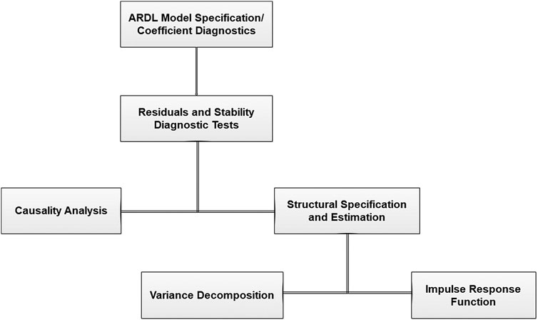
FIGURE 1. Model Framework.

Results and Discussion

Statistical Analysis

The mean of the variables showed that incomes have the highest meanwhile CO₂ emissions and biocapacity have low and negative mean scores. The standard deviations are also low with energy use having the lowest. This suggests that all the variables are less volatile over the study period. The skewness of the variables indicates that CO₂ emissions and biocapacity are negatively skewed while income, the squared term of income, agriculture, and energy use are positively skewed with the values tending toward zero. More so, the kurtosis of the variables indicated that all the series have a positive kurtosis with Jarque-Bera values exceeding the region of normal distribution as can be seen by the probability values.

The graphical plots of the variables in described in Figure 2. This is necessitated by the presence of drift, trend, and seasonality as well as structural breaks. As shown by the Figure, all the variables seem to have structural breaks. These breaks are more evident in CO₂ emissions, biocapacity, and energy use with no precise evidence of a trend. For income, squared income, and agriculture, it is observed that the variables begin to trend upward.

FIGURE 2

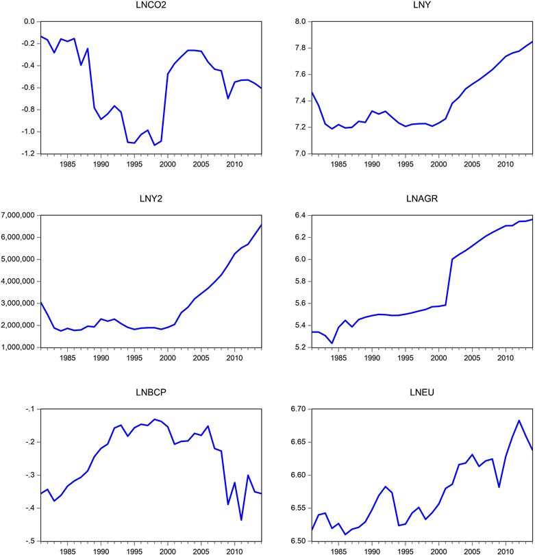
FIGURE 2. Natural logarithms of CO₂, Y, Y², AGR, BCP, and EU.

Stationary Test Results

Before estimating the model for this study, we first, applied the usual unit root tests via ADF and PP as earlier stated. The results given in Table 2, Panel A show that all the series (CO₂ emissions, Income, the square of income, agricultural innovation, biocapacity, and energy use) are not stationary in their levels. However, after we took their first differences, they all turn out to be stationary. This means that the variables are classified as I (1) process. To circumvent the inadequacy of conventional unit root tests, we applied the minimum LM unit root test with one break. The results as displayed in Table 2, Panel B validated the earlier results that all the series are integrated of order one, i.e., I (1) process. Also, the identified breakpoint for CO₂ emissions is 1999, income and its squared term is 2006; agricultural value added is 2001, biocapacity is 2010, and energy use is 2002. The break in 1999 could be attributed to the effect of general elections which lowers the pressure on stimulating growth and hence CO₂ emissions. The break in 2002 may be caused by the effect of pre-2003 general elections. The 2006 break in income and its squared term can be attributed to exchange rate volatility, which significantly affected income levels. Finally, the 2010 break was caused by 2008 worldwide financial disaster which affected the agricultural sector significantly.

TABLE 2

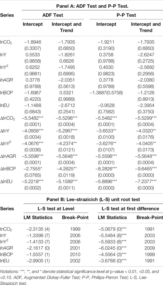
TABLE 2. Augmented Dickey-Fuller (ADF), Phillips-Perron (P-P) and Lee-Strazicich (L-S) Unit Root tests.

TABLE 3

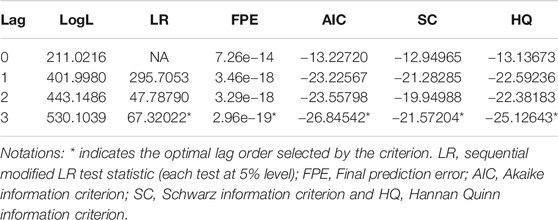
TABLE 3. VAR optimal lag order selection criteria.

Co-Integration Tests

Having established the integrating properties of the variables in our model, the next is to check whether co-integration exists among the variables. To do this, we applied the ARDL bounds testing approach. The robustness of this test is carried out based on the combined cointegration test (Bayer and Hanck, 2013). The lag length selection of three based on the Akaike information criterion (AIC) is shown in Table 3 while Table 4 provided the reports of the bounds-testing co-integration. According to the reports, we found that when each of the variables is treated as endogenous, we confirmed five co-integrating vectors, which by implication means that a long-run relationship exists between the sampled series. These findings are validated by the combined co-integration test of Bayer-Hanck Table 5, which found a co-integration in all the six equations, implying that there is a long-run nexus between the investigated series.

TABLE 4

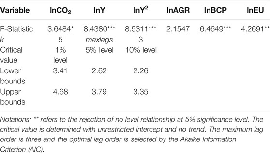
TABLE 4. Estimates of ARDL bounds test for cointegration.

TABLE 5

TABLE 5. Estimates of cointegration test via Bayer-Hanck.

ARDL Estimated Results

Table 6 reports the long-run and short-run parameters of the ARDL model estimator. Based on the parameters of the model, we find evidence that real income and its squared term have a positive and negative relationship with CO₂ in the long run and short run, respectively. The negative effect of squared term of income indicates a breakaway of CO₂ emissions and real income at higher income level. This result, therefore, suggests the validation of the EKC hypothesis in Nigeria both in the long run and short run. The plausible reason for the findings is that Nigeria being an oil-exporting country mostly engages in excessive use of fossil fuels and cement manufacturing. Furthermore, a larger carbon is emitted during the utilization of liquid and gas fuels as well as gas flaring. Therefore, the validity of the EKC hypothesis in this study is consistent with previous studies such as Galeotti et al., (2006), Shahbaz et al. (2013), Shahbaz et al. (2017), Usman et al. (2019, 2020), Agboola and Bekun (2019), Ike (2020a, 2020b, 2020c), Iorember et al. (2020). The effect of agricultural innovation on CO₂ emissions is positive, inelastic, and statistically significant both in the long run and short run. This implies that a 1% increase in agricultural innovation would cause CO₂ emissions to rise by 0.5145% in the long run and 0.5329% in the short run. The economic reason supporting this result is that agricultural practices such as bush burning, tillage, fertilization, deforestation, and desertification as well as raising livestock like cattle, pigs, fish and poultry could accelerate the level of anthropogenic carbon emissions. This finding agrees with a study that found a positive relationship between agriculture and CO₂ emissions in Nigeria (Agboola and Bekun, 2019). Our result also corroborates with Olanipekun et al. (2019) who found a similar result for African countries and for Tunisia (Ben Jebli and Ben Youssef, 2017). Moreover, we found that after taking the first lag of agricultural value-added, its effect on CO₂ emissions was negative, indicating that the historical effects of agricultural value-added underpin CO₂ emissions mitigation. The negative relationship between agriculture and CO₂ emissions is supported by a finding documented for 53 countries in the world (Rafiq et al., 2016); five MENA countries (Ben Jebli and Ben Youssef, 2017), and Turkey (Dogan, 2016).

TABLE 6

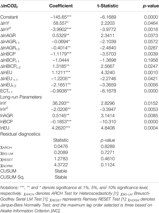
TABLE 6. ARDL parameter estimates.

Furthermore, the influence of biocapacity on CO₂ emissions is negative, inelastic and substantial in the long run while in the short run, it is negative, elastic and significant. Particularly, a 1% increase in biocapacity would reduce CO₂ emissions by 0.1853% in the long run, while in the short run, it reduces CO₂ emissions by 1.1179%. This is because biocapacity is a non-carbon measurement of the ability of the ecosystem to renew the biological materials demand by the people from the earth’s surfaces. Therefore, it is consistent with the Sarkodie and Strezov (2018) who found a negative relationship between biocapacity and CO₂ emissions for the US, Australia, China and Ghana. Finally, the influence of energy use is positive, elastic and statistically significant with CO₂ emissions. This means that a 1% increase in energy use would increase CO₂ emissions by 4.2620% in the long run and 1.1211% in the short run. The results further showed that from one lag period afterward, the effect of energy use on CO₂ emissions turns negative. The implication for this result is that most of the Nigerian energy sources are stemming traditional biomass and waste, which could explain about 83% of the total primary production, while 16% is accounted for by the fossil fuels and 1% by hydropower. These energy sources are renewables, which emit low carbon and GHGs. This reason is also attributed to the negative effects of agriculture from the first lag afterward.

The speed of adjustment (ECT_t-1) is negative and significant with a value −0.9938. This implies that the speed of convergence from short-run variation toward equilibrium long run is about 99% yearly. We also tested the diagnostics of the model estimated. The results showed that there is no case of serial correlation and conditional heteroscedasticity problems. Similarly, the functional form of the model is correctly constructed with evidence that the error term is normally distributed. Furthermore, apart from the RAMSEY RESET test, we applied the cumulative sum (CUSUM) and CUSUM squares (CUSUM Sq.) to test the stability of the model. As shown in Figure 3, both tests revealed that the model is stable and adequate both in the long and short run.

FIGURE 3

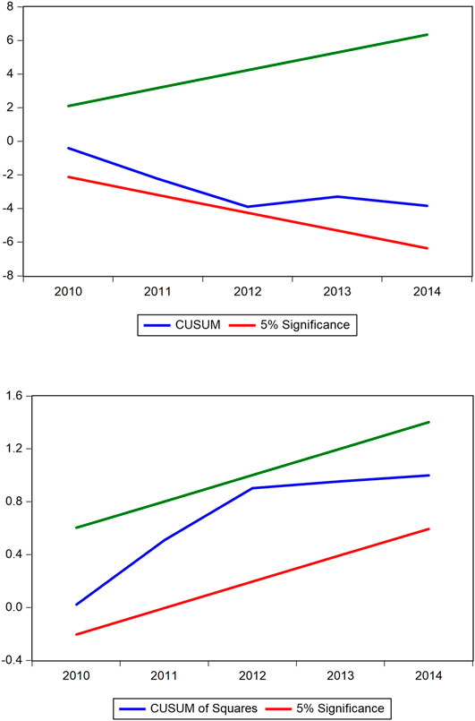
FIGURE 3. Plot of cumulative sum (CUSUM) and cumulative sum of squares (CUSUM Sq.) at 5% significance.

Causality and Innovation Accounting

Theoretically, if a co-integration is found, there must be at least causality between the variable. As displayed in Table 7, we found evidence that a uni-directional causality runs from agriculture to CO₂ emissions, which contradicts the earlier finding by Agboola and Bekun (2019). The plausible reason could be attributed to the fact that the study applied a standard Granger causality which tends to produce a spurious result if the variables are not all integrated at levels. However, our finding agrees with Ben Jebli and Ben Youssef (2017) who found agriculture and CO₂ emissions to have a causal link in the long run for five MENA countries. We also found that CO₂ emission could predict income, biocapacity, and energy use. Furthermore, our results provide evidence that a bidirectional causal relationship exists between agriculture and biocapacity as well as agriculture and energy use. These results imply that agriculture causes biocapacity and energy use and vice versa. The results that agriculture has predictability for energy use are consistent with Agboola and Bekun (2019). This is also consistent with Ben Jebli and Ben Youssef (2017) who found a long-run causality running from renewable energy to agriculture. There is also evidence that income level and its squared term have predictability for energy use. This result also corroborates a similar reported case in Ben Jebli and Ben Youssef (2017).

TABLE 7

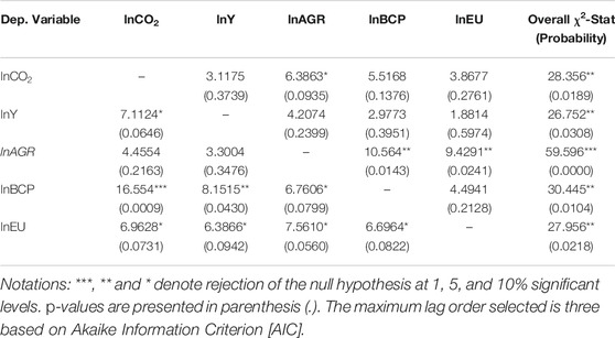
TABLE 7. Result of causal relationship test.

We step forward to validate our findings via the innovation accounting test of variance decomposition and impulse—response function analyses based on 10-year forecast horizons. From Table 8, we found that except for energy use, CO₂ emissions have the highest contribution to the variance decomposition of all the variables in the model. Similarly, energy use has the lowest contribution to the variance decomposition of all the variables. Starting from the variance decomposition of CO₂ emissions, we observed that own shock contributed about 65.4%, followed by the contribution from agriculture which accounted for about 11.65%. Energy use has the lowest contribution of 1.46%, which confirms the earlier results that about 83% of total energy consumption in Nigeria stems from the renewables which emit low carbon dioxide. More so, from the variance decomposition of income and its squared term, we found that CO₂ emissions contributed about 56.01 and 56.4%. This is followed by the contribution of agriculture, which accounted for about 22.8 and 22.7%, respectively. The contribution of energy use is about 1.60%. We further found that while agriculture contributed about 32.01% due to own shock, the contribution of CO₂ emissions is about 49.42% while energy use is about 2.41%. The results further suggested that for variance decomposition of bio-capacity, own shock contributed just 13.23% while CO₂ emissions contributed about 35.78% with 1.71% contribution from energy use. Additionally, the highest contributor to the variance decomposition of energy use is squared term of income with about 31.24%, apparently followed by agriculture with about 23.09%. The contribution from its own shock is about 3.83%. Therefore, from the results of the forecast error variance decomposition, we observed that 22.79% of agriculture corresponded to 49.43% CO₂ emissions. We also found that 5.95% biocapacity caused 35.78% CO₂ emissions, while 1.61% of energy use led to just 16.27% CO₂ emissions.

TABLE 8

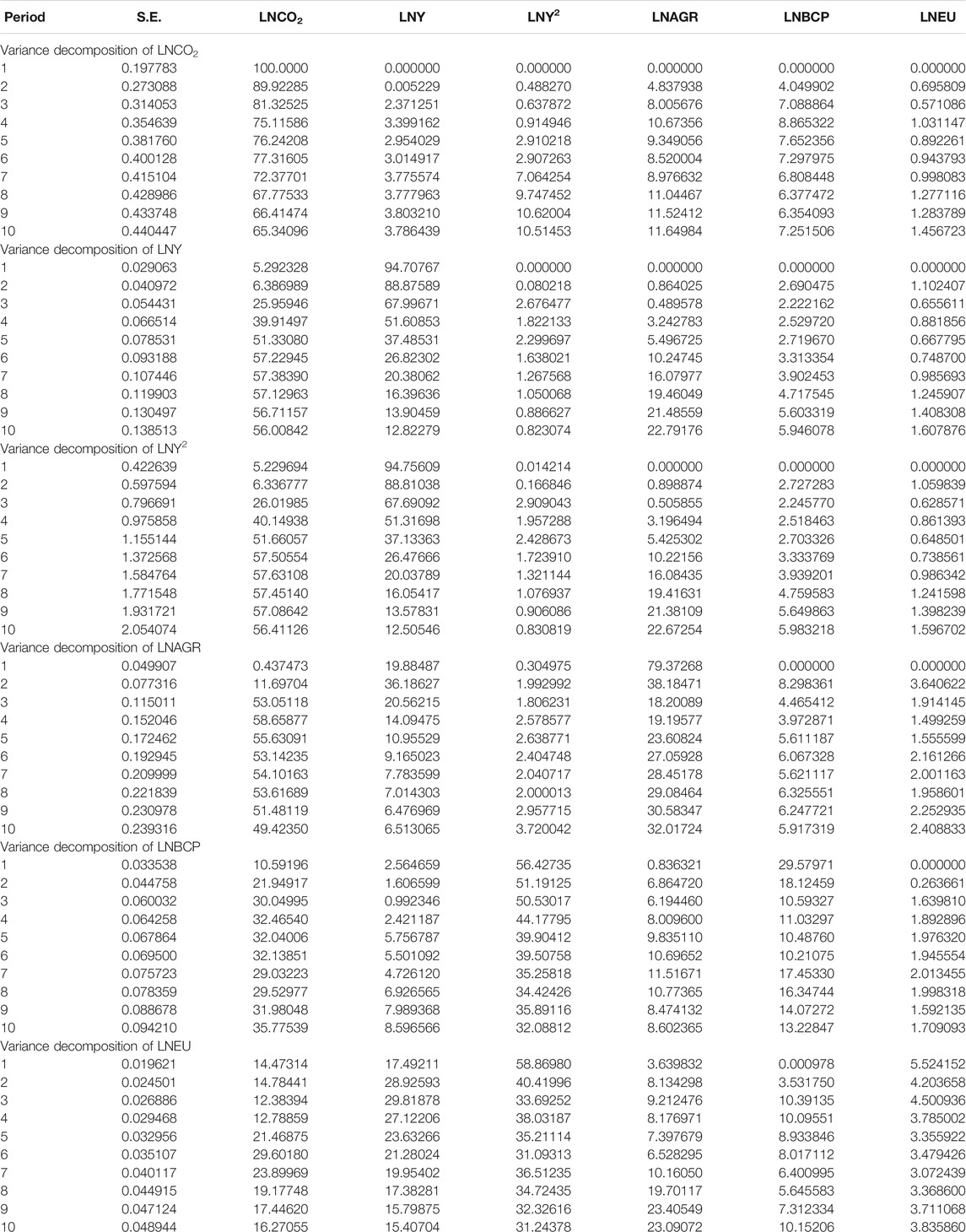
TABLE 8. Forecast error variance decomposition.

Figure 4 presents the impulse responses of all the variables to an innovation shock. As shown, CO₂ emissions responded positively to the innovation shocks up to the eighth horizons and consequently turned negative. This implies that about 8th horizons, CO₂ emissions responds negatively to innovation shocks. For income, we found that the response of income to innovation shocks is positive until sixth horizon. The response became negative between sixth and eighth horizons, after which it became positive. The same is not observed in the case of income squared. The response of the square of income is positive with no visible evidence of a trend (i.e., response moves ups and downs) until it became negative after the sixth horizons. The response of agriculture to innovation shocks is positive over the periods of horizons, while that of biocapacity is characterized by upward and downward movements over the entire horizons. Finally, the response of energy use to innovation is positive up to the fourth horizon. However, between fourth and sixth horizons, the response turned negative and consequently crossed to the positive region in the mid-sixth horizons. The results have validated the causality we have found between the variables.

FIGURE 4

FIGURE 4. Impulse Response Functions (IMFs).

Counterfactual Change

The traditional ARDL estimation procedure produces in-sample parameters that often complicate for statistical inferences. The novel dynamic ARDL simulations technique was developed by Jordan and Philips (2018) and utilized in the seminal work of Sarkodie et al. (2019). The versatility and policy usefulness of the estimation method has been applied in several disciplines (Owusu and Sarkodie, 2020b; Sarkodie et al., 2020; Shabbir et al., 2020). Thus, we utilized the novel dynamic ARDL simulations to examine the out-sample effects of counterfactual shocks in exogeneous independent variable at a given time period. This is appropriate to examine how CO₂ emissions will respond to future shocks from a specified exogeneous regressor. The counterfactual shocks observed in Figures 5A,B reveals that −1% change in predicted income has no potential effect in the first 9 years but a 1.4% positive rebound effect of CO₂ emissions is observed in the 10th year and stabilizes from the 13th year and thereafter. Contrary, a 1.4% negative rebound effect is observed after 10 years of 1% shock in predicted income but turns steady after 13 years. This implies that wealth has a long-term mitigating effect on CO₂ emissions—corroborating the notion of pollute in poverty, clean when wealthy.

FIGURE 5

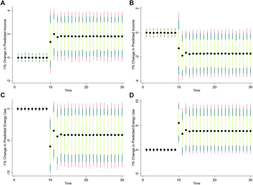
FIGURE 5. Counterfactual shocks (A) −1% Change in Predicted Income (B) 1% Change in Predicted Income (C) −1% Change in Predicted Energy Use (D) 1% Change in Predicted Energy Use. Legend: The filled-black circle denotes the predicted shock whereas sunflower lime, emerald and cranberry colored spikes refer to statistical significance at 25, 10, 5% level.

A similar trend is observed in Figures 5C,D, however, −1% shock in predicted energy utilization leads to over 5% decline in CO₂ emissions from the 10th year but reaches a steady-state in the 14th year and afterward. In contrast, over 5% increase in CO₂ emissions is observed after 9 years of no impact at a 1% change in energy consumption. Thus, energy intensity has an escalation effect on CO₂ emissions, which calls for energy efficiency, management, and conservation options to decarbonize energy utilization. Unlike income and energy utilization, there is evidence of very little impact (∼0.001%) observed in CO₂ emissions at −1% change in predicted agricultural innovation in the first 10 years. However, a sharp decline of CO₂ emissions by 0.48% is noticed in the 11th year but a “noisy” effect of reduction in CO₂ is observed thereafter. A 1% shock in predicted agricultural innovation escalates CO₂ emissions by 0.47% from the 11th year and afterward (Figures 6A,B). The relatively low impact of agricultural innovation on CO₂ emissions compared to energy utilization—can be attributed to vintage agricultural practices, mechanization, and technologies for value addition. This implies that the implementation of modernized and sustainable agricultural process may have a long-term effect, leading to a decarbonized agrarian economy.

FIGURE 6

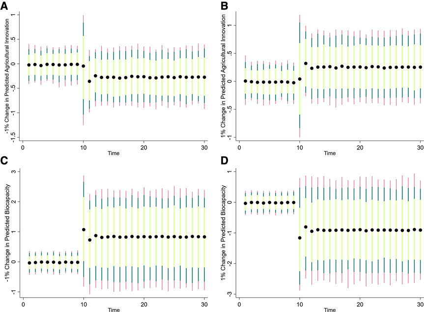
FIGURE 6. Counterfactual shocks (A) −1% Change in Predicted Agricultural Innovation (B) 1% Change in Predicted Agricultural Innovation (C) −% Change in Predicted Biocapacity (D) 1% Change in Predicted Biocapacity. Legend: The filled-black circle denotes the predicted shock whereas sunflower lime, emerald and cranberry colored spikes refer to statistical significance at 25, 10, 5% level.

Regeneration of the ecosystem plays an essential role in reducing carbon footprint. We observe in Figures 6C,D that −1% shock in predicted biocapacity increases CO₂ emissions by almost 1% after 9 years whereas 1% change in predicted biocapacity declines CO₂ emissions by ∼1%. Implying that a reduction in ecological footprint will improve the regenerative capacity of the ecosystem, hence, reducing emissions in the long-term.

Conclusion and Policy Implications

Agrarian-based economies are often characterized by natural resource exploitation and ecological degradation. In this study, we assessed the impact of agricultural innovation and biocapacity on carbon-based emissions and tested the validity of the EKC hypothesis in Nigeria. We applied several estimation techniques including the novel dynamic ARDL simulations, with data from 1981 to 2014. The empirical evidence based on the ARDL procedure confirmed the long- and short-run validity of the EKC hypothesis for Nigeria. We found that agricultural innovation and energy utilization escalate the levels of anthropogenic CO₂ emissions. In contrast, an expansion of the regenerative capacity of the ecosystem is found to decline the outgrowth of CO₂ emissions. The causality revealed that agricultural innovation has strong predictive power on CO₂ emissions. Similarly, we found income level to predict long-term energy utilization. The results indicated that CO₂ emissions predict income, biocapacity and energy use while feedback causality occurs between agriculture and biocapacity and again agriculture and energy use. These findings were validated by the variance decomposition and impulse-response function analyses. Particularly, we found that 22.79% of agricultural innovation corresponds to 49.43% CO₂ emissions. We also found that 5.95% biocapacity caused 35.78% CO₂ emissions, while 1.61% of energy use led to just 16.27% CO₂ emissions. In contrast to the in-sample estimation techniques, the counterfactual shocks from the novel dynamic ARDL simulation showed favourable mitigation effects of income, and biocapacity on CO₂ emissions whereas escalation effects of agricultural innovation and energy utilization were also noticed. These findings demonstrate that improvement in livelihoods, environmental awareness creation, and prioritization of ecosystem management and restoration will have a long-term effect on environmental sustainability.

Therefore, based on these findings, to achieve carbon sequestration in Nigeria, there is a need for sustainable and clean energy policies that have low environmental damaging effects. Such policies would discourage the excessive use of traditional biomass and fossil fuels. Second, decarbonizing agricultural innovations will include sustainable agricultural practices that encourage clean and renewable energy utilization for agricultural activities. For example, solar energy can be extended to greenhouse heating and cooling, product drying and lighting, in addition to irrigation in the farm field. More so, for improvement in soil, greenhouse, and barns, as well as heating the soil and drying agricultural products, geothermal can be applied. Furthermore, bioenergy can be used to power machinery whereas wind and hydro can be used to generate electricity, irrigate, and process crops. In addition to the above, we suggest a number of policy instruments to mitigate carbon dioxide emissions in Nigeria. These instruments include the use of fiscal instruments such as taxes and fees. We also suggest that financial instruments like subsidies can also be used to regulate the behaviors of the polluters. The coercive power of the state can be applied on polluters who go beyond the avoidable levels of pollution as prescribed by industrial emission standards.

To this end, future studies can shift from theoretical investigation to undertake a randomized controlled trial that examines the effect of sustainable agricultural practices on CO₂ emissions. Such experimental studies will improve the global debate on emissions.

Data Availability Statement

Publicly available datasets were analyzed in this study. This data can be found here: https://databank.worldbank.org/reports.aspx?source=World-Development-Indicators. All scripts from the estimation method are available upon reasonable request.

Author Contributions

AA: Supervising and editing-original draft. MU: Writing and editing- original draft. OU: Conceptualization, Formal analysis, Investigation, Methodology. SS: Writing - review & editing, Funding acquisition, Validation, Visualization.

Funding

Open Access funding provided by Nord University.

Conflict of Interest

The authors declare that the research was conducted in the absence of any commercial or financial relationships that could be construed as a potential conflict of interest.

Footnotes

¹Some of the data employed are only available up to 2014 for the case of Nigeria.

²https://buff.ly/2DkRfOb

³https://buff.ly/3gWbT5T

⁴“The capacity of ecosystems to regenerate what people demand from those surfaces. Life, including human life, competes for space. The biocapacity of a surface represents its ability to renew what people demand. Biocapacity is, therefore, the ecosystems’ capacity to produce biological materials used by people and to absorb waste material generated by humans, under current management schemes and extraction technologies. Biocapacity can change from year to year due to climate, management, and proportion considered useful inputs to the human economy”. We follow the National Footprint Accounts, where biocapacity is calculated by “multiplying the physical area by the yield factor and the appropriate equivalence factor. Biocapacity is expressed in global hectares” (Global Footprint Network, 2017).

References

Agboola, M. O., and Bekun, F. V. (2019). Does agricultural value added induce environmental degradation? Empirical evidence from an agrarian country. Environ. Sci. Pollut. Res. Int. 26 (27), 27600–27676. doi:10.1007/s11356-019-05943-z

CrossRef Full Text | Google Scholar

Apergis, N. (2016). Environmental Kuznets curves: new evidence on both panel and country-level CO₂ emissions. Energy Econ. 54, 263–271. doi:10.1016/j.eneco.2015.12.007

CrossRef Full Text | Google Scholar

Bayer, C., and Hanck, C. (2013). Combining non-cointegration tests. J. Time Anal. 34 (1), 83–95. doi:10.1111/j.1467-9892.2012.00814.x

CrossRef Full Text | Google Scholar

Ben Jebli, M., and Ben Youssef, S. (2017). Renewable energy consumption and agriculture: evidence for cointegration and Granger causality for Tunisian economy. Int. J. Sustain. Dev. World Ecol. 24 (2), 149–158. doi:10.1080/13504509.2016.1196467

CrossRef Full Text | Google Scholar

Blanco, A. S., Gerlagh, R., Suh, S., Barrett, J. A., de Coninck, H., Diaz Morejon, C. F., et al. (2014). “Drivers, trends and mitigation.” in Climate change 2014: mitigation of climate change. Cambridge, United Kingdom: Cambridge University Press.

Google Scholar

Dogan, N. (2016). Agriculture and environmental Kuznets curves in the case of Turkey: evidence from the ARDL and bounds test. Agric. Econ. 62 (12), 566–574. doi:10.17221/112/2015-AGRICECON

CrossRef Full Text | Google Scholar

United States Food and Agricultural Organization (FAO) (2016). Available at: http://www.fao.org/3/a-i6030e.pdf (Accessed August 6, 2020).

Google Scholar

Fried, B., and Getzner, M. (2003). Determinants of CO₂ emissions in a small open economy. Ecol. Econ. 45, 133–148. doi:10.1016/S0921-8009(03)00008-9

CrossRef Full Text | Google Scholar

Galeotti, M., Lanza, A., and Pauli, F. (2006). Reassessing the environmental Kuznets curve for CO₂ emissions: a robustness exercise. Ecol. Econ. 57 (1), 152–163. doi:10.1016/j.ecolecon.2005.03.031

CrossRef Full Text | Google Scholar

Global Footprint Network (2017). Ecological footprint. Available at: http://www.footprintnetwork.org.

CrossRef Full Text | Google Scholar

Gokmenoglu, K. K., and Taspinar, N. (2018). Testing the agriculture-induced EKC hypothesis: the case of Pakistan. Environ. Sci. Pollut. Res.Int. 25 (23), 22829–22841. doi:10.1007/s11356-018-2330-6

PubMed Abstract | CrossRef Full Text | Google Scholar

Grossman, C., and Krueger, A. B. (1991). Environmental impacts of a north American free trade agreement. NBER, Working Paper Number 3914.

CrossRef Full Text | Google Scholar

HEI (2018). Health effect institute reports. Available at:https://www.healtheffects.org/ (Accessed August 6, 2020).

Google Scholar

Ike, G. N., Usman, O., and Sarkodie, S. A. (2020a). Testing the role of oil production in the environmental Kuznets curve of oil producing countries: new insights from method of moments quantile regression. Sci. Total Environ. 711, 135208. doi:10.1016/j.scitotenv.2019.135208

PubMed Abstract | CrossRef Full Text | Google Scholar

Ike, G. N., Usman, O., and Sarkodie, S. A. (2020b). Fiscal policy and CO2 emissions from heterogeneous fuel sources in Thailand: evidence from multiple structural breaks cointegration test. Sci. Total Environ. 702, 134711. doi:10.1016/j.scitotenv.2019.134711

PubMed Abstract | CrossRef Full Text | Google Scholar

Ike, G. N., Usman, O., Alola, A. A., and Sarkodie, S. A. (2020c). Environmental quality effects of income, energy prices and trade: the role of renewable energy consumption in G-7 countries. Sci. Total Environ. 721, 137813. doi:10.1016/j.scitotenv.2020.137813

PubMed Abstract | CrossRef Full Text | Google Scholar

Inglesi-Lotz, R., and Bohlmann, J. (2014). Environmental Kuznets curve in South Africa: to confirm or not to confirm? Prepared for Ecomod, 2014. Bali, Indonesia.

Google Scholar

Intergovernmental Panel on Climate Change (IPCC) (2017). Available at: https://www.ipcc.ch/report/ (Accessed August 6, 2020).

Google Scholar

Iorember, P. T., Goshit, G. G., and Dabwor, D. T. (2020). Testing the nexus between renewable energy consumption and environmental quality in Nigeria: the role of broad‐based financial development. Afr. Dev. Rev. 32 (2), 163–175. doi:10.1111/1467-8268.12425

CrossRef Full Text | Google Scholar

Jordan, S., and Philips, A. Q. (2018). Cointegration testing and dynamic simulations of autoregressive distributed lag models. STATA J. 18 (4), 902–923. doi:10.1177/1536867X1801800409

CrossRef Full Text | Google Scholar

Kasman, A., and Duman, Y. S. (2015). CO₂ emissions, economic growth, energy consumption, trade and urbanization in new EU member and candidate countries: a panel data analysis. Econ. Modell. 44, 97–103. doi:10.1016/j.econmod.2014.10.022

CrossRef Full Text | Google Scholar

Kuznets, S. (1955). Economic growth and income inequality. Am. Econ. Rev. 45 (1), 1–28.

Google Scholar

Lee, J., and Strazicich, M. C. (2003). Minimum Lagrange multiplier unit root test with two structural breaks. Rev. Econ. Stat. 85 (4), 1082–1089.

CrossRef Full Text | Google Scholar

Liu, X., Zhang, S., and Bae, J. (2017). The nexus of renewable energy-agriculture environment in BRICS. Appl. Energy 204, 489–496. doi:10.1016/j.apenergy.2017.07.077

CrossRef Full Text | Google Scholar

Mesagan, E. P., Isola, W. A., and Ajide, K. B. (2018). The capital investment channel of environmental improvement: evidence from BRICS. Environ. Dev. Sustain. 21 (4), 1561–1582. doi:10.1007/s10668-018-0110-6

CrossRef Full Text | Google Scholar

Narayan, P. K., and Narayan, S. (2010). Carbon dioxide emissions and economic growth: panel data evidence from developing countries. Energy Policy 38 (1), 661–666. doi:10.1016/j.enpol.2009.09.005

CrossRef Full Text | Google Scholar

Nasr, A. B., Gupta, R., and Sato, J. R. (2015). Is there an environmental Kuznets curve for South Africa? A Co-summability approach using a century of data. Energy Econ. 52, 136–141. doi:10.1016/j.eneco.2015.10.005

CrossRef Full Text | Google Scholar

Olanipekun, I. O., Olasehinde-Williams, G. O., and Alao, R. O. (2019). Agriculture and environmental degradation in Africa: the role of income. Sci. Total Environ. 692, 60–67. doi:10.1016/j.scitotenv.2019.07.129

PubMed Abstract | CrossRef Full Text | Google Scholar

Owusu, P. A., and Asumadu, S. S. (2016). Is there a causal effect between agricultural production and carbon dioxide emissions in Ghana? Environ. Eng. Res. 22 (1), 40–54. doi:10.4491/eer.2016.092

CrossRef Full Text | Google Scholar

Owusu, P. A., and Sarkodie, S. A. (2020a). Global estimation of mortality, disability-adjusted life years and welfare cost from exposure to ambient air pollution. Sci. Total Environ. 742, 140636. doi:10.1016/j.scitotenv.2020.140636

PubMed Abstract | CrossRef Full Text | Google Scholar

Owusu, P. A., and Sarkodie, S. A. (2020b). How to apply the novel dynamic ARDL simulations (dynardl) and Kernel-based regularized least squares (krls). MethodsX 7, 101160. doi:10.1016/j.mex.2020.101160

Perron, P. (1989). The great crash, the oil price shock, and the unit root hypothesis. Econometrica: J. Econometric Soc. 1361–1401.

Pesaran, M. H., Shin, Y., and Smith, R. J. (2001). Bounds testing approaches to the analysis of level relationships. J. Appl. Econ. 16 (3), 289–326. doi:10.1002/jae.616

CrossRef Full Text | Google Scholar

Rafindadi, A. A., and Usman, O. (2019). Globalization, energy use, and environmental degradation in South Africa: startling empirical evidence from the Maki-cointegration test. J. Environ. Manag. 244, 265–275. doi:10.1016/j.jenvman.2019.05.048

CrossRef Full Text | Google Scholar

Rafindadi, A. A. (2016). Revisiting the concept of environmental Kuznets curve in period of energy disaster and deteriorating income: empirical evidence from Japan. Energy Pol. 94, 274–284. doi:10.1016/j.enpol.2016.03.040

CrossRef Full Text | Google Scholar

Rafiq, S., Salim, R., and Apergis, N. (2016). Agriculture: trade openness and emissions: an empirical analysis and policy options. Aust. J. Agric. Resour. Econ. 60, 348–365. doi:10.1111/1467-8489.12131

CrossRef Full Text | Google Scholar

Reynolds, L., and Wenzlau, S. (2012). Climate-friendly agriculture and renewable energy: working hand-in-hand toward climate mitigation. Worldwatch InstituteAvailable at: http://www.renewableenergyworld.com/articles/2012/12/climate-friendly-agriculture-and-renewable-energy-working-hand-inhandtoward-climate-mitigation.html (Accessed August 6, 2020).

Google Scholar

Sarkodie, S. A., Adams, S., Owusu, P. A., Leirvik, T., and Ozturk, I. (2020). Mitigating degradation and emissions in China: the role of environmental sustainability, human capital and renewable energy. Sci. Total Environ. 719, 137530. doi:10.1016/j.scitotenv.2020.137530

PubMed Abstract | CrossRef Full Text | Google Scholar

Sarkodie, S. A., Strezov, V., Weldekidan, H., Asamoah, E. F., Owusu, P. A., and Doyi, I. N. Y. (2019). Environmental sustainability assessment using dynamic Autoregressive-Distributed Lag simulations-Nexus between greenhouse gas emissions, biomass energy, food and economic growth. Sci. Total Environ. 668, 318–332. doi:10.1016/j.scitotenv.2019.02.432

PubMed Abstract | CrossRef Full Text | Google Scholar

Sarkodie, S. A., Ntiamoah, E. B., and Li, D. (2019). Panel heterogeneous distribution analysis of trade and modernized agriculture on CO₂ emissions: the role of renewable and fossil fuel energy consumption. Nat. Resour. Forum. 43, 135–153. doi:10.1111/1477-8947.12183

CrossRef Full Text | Google Scholar

Sarkodie, S. A., and Strezov, V. (2018). Empirical study of the environmental Kuznets curve and environmental sustainability curve hypothesis for Australia, China, Ghana and USA. J. Clean. Prod. 201, 98–110. doi:10.1016/j.jclepro.2018.08.039

CrossRef Full Text | Google Scholar

Selden, T. M., and Song, D. (1994). Environmental quality and development: is there a Kuznets curve for air pollution emissions? J. Environ. Econ. Manag. 27 (2), 147–162. doi:10.1006/jeem.1994.1031

CrossRef Full Text | Google Scholar

Shabbir, A. H., Zhang, J., Johnston, J. D., Sarkodie, S. A., Lutz, J. A., and Liu, X. (2020). Predicting the influence of climate on grassland area burned in Xilingol, China with dynamic simulations of autoregressive distributed lag models. PLoS One 15 (4), e0229894. doi:10.1371/journal.pone.0229894

PubMed Abstract | CrossRef Full Text | Google Scholar

Shahbaz, M., Farhani, S., and Ozturk, I. (2014). Do coal consumption and industrial development increase environmental degradation in China and India? Environ. Sci. Pollut. Res. Int. 22 (5), 3895–3907. doi:10.1007/s11356-014-3613-1

PubMed Abstract | CrossRef Full Text | Google Scholar

Shahbaz, M., Khan, S., Ali, A., and Bhattacharya, M. (2017a). The impact of globalization on CO₂ emissions in China. Singapore Econ. Rev. 62 (4), 929–957. doi:10.1142/S0217590817400331

CrossRef Full Text | Google Scholar

Shahbaz, M., Ozturk, I., Afza, T., and Ali, A. (2013). Revisiting the environmental Kuznets curve in a global economy. Renew. Sustain. Energy Rev. 25, 494–502. doi:10.1016/j.rser.2013.05.021

CrossRef Full Text | Google Scholar

Spangenberg, J. H. (2001). The environmental Kuznets curve: a methodological artefact? Popul. Environ. 23 (2), 175–191. doi:10.1023/A:1012827703885

CrossRef Full Text | Google Scholar

Tiwari, A. K., Shahbaz, M., and Hye, Q. M. A. (2013). The environmental Kuznets curve and the role of coal consumption in India: cointegration and causality analysis in an open economy. Renew. Sustain. Energy Rev. 18, 519–527. doi:10.1016/j.rser.2012.10.031

CrossRef Full Text | Google Scholar

Toda, H. Y., and Yamamoto, T. (1995). Statistical inference in vector autoregressions with possibly integrated processes. J. Econom. 66 (1), 225–250. doi:10.1016/0304-4076(94)01616-8

CrossRef Full Text | Google Scholar

Usman, O., Iorember, P. T., and Olanipekun, I. O. (2019). Revisiting the environmental Kuznets curve (EKC) hypothesis in India: the effects of energy consumption and democracy. Environ. Sci. Pollut. Res. Int. 26 (13), 13390–13400. doi:10.1007/s11356-019-04696-z

PubMed Abstract | CrossRef Full Text | Google Scholar

Usman, O., Alola, A. A., and Sarkodie, S. A. (2020a). Assessment of the role of renewable energy consumption and trade policy on environmental degradation using innovation accounting: evidence from the US. Renew. Energy 150, 266–277. doi:10.1016/j.renene.2019.12.151

CrossRef Full Text | Google Scholar

Usman, O., Olanipekun, I. O., Iorember, P. T., and Abu-Goodman, M. (2020b). Modelling environmental degradation in South Africa: the effects of energy consumption, democracy, and globalization using innovation accounting tests. Environ. Sci. Pollut. Res. Int. 27, 8334–8349. doi:10.1007/s11356-019-06687-6

PubMed Abstract | CrossRef Full Text | Google Scholar

World Bank (2015). World Bank database. Available at: https://datacatalog.worldbank.org/dataset/world-development-indicators (Accessed August 6, 2020).

Google Scholar