 Shouxiang Wang
 Kaixin Wu1
 Qianyu Zhao
- 1Key Laboratory of the Ministry of Education on Smart Power Grids, Tianjin University, Tianjin, China
- 2State Grid Shandong Economic and Technological Research Institute, Jinan, China
- 3Lanzhou Jiaotong University, Lanzhou, China
Multienergy load forecasting (MELF) is the premise of regional integrated energy systems (RIES) production planning and energy dispatch. The key of MELF is the consideration of multienergy coupling and the improvement of prediction accuracy. Therefore, a MELF method considering the multienergy coupling of variation characteristic curves (MELF_MECVCC) for RIES is proposed. The novelty of MELF_MECVCC lies in the following three aspects. 1) For the trend stripping and volatility extraction of multienergy load time series, the extreme-point symmetric mode decomposition-sample entropy (ESMD-SE) method is introduced to decompose and reconstruct the variation characteristic curves of multienergy, including trend curve and fluctuation curve. 2) The multienergy coupling of the variation characteristic curves is considered to reflect the variation characteristics of the multienergy loads. 3) Different methods are applied according to different variation characteristics; i.e., the combined method based on multitask learning and long short-term memory network (MTL-LSTM) is applied to predict the trend curve with strong correlation and the least square support vector regression (LSSVR) method is applied to predict the fluctuation curve with strong volatility and high complexity. Based on the actual data set of the University of Texas in Austin, the MELF_MECVCC model is simulated and verified, which shows that the model reduces the mean absolute percentage error (MAPE) and the root mean square error (RMSE) and fits better with the original load and has higher prediction accuracy, compared with current advanced algorithms.
Introduction
The RIES utilize the advanced technology of physical information systems and innovative management models to integrate a variety of heterogeneous energy sources such as electricity, heating, and cooling in a certain area to realize coordinated planning, management, and optimized operation of diversified energy. Compared with the traditional single-energy systems, RIES integrate diversified forms of energy supply, conversion, and storage equipment, which improve the coupling of different types of energy in different links such as source, network, and load, and also improve the flexibility of the overall system energy consumption (Shi et al., 2018). They are important parts of the new generation energy systems to build clean, low-carbon, safe, and efficient modern energy systems. In 2008, the United States launched the FREEDM project, expecting to use the technology of power electronics, information, and intelligent management to build an energy peer-to-peer exchange and sharing network (Yuan et al., 2019). In October 2017, the State Grid Corporation of China issued a document to promote the company’s transformation from an electricity supplier to an integrated energy service provider. Therefore, with the promotion and development of RIES, load forecasting is an important prerequisite for the optimization and management of energy systems, and its accuracy, reliability, and intelligence are given higher requirements. At the same time, considering the coupling of diversified energy sources has become one of the key points of load forecasting.
Since load forecasting plays a vital role in energy management and optimized operation of RIES and traditional single-energy systems, a lot of research work has been done on this topic. Traditional load forecasting methods can be classified into two categories: traditional methods and artificial intelligence methods. Traditional methods are represented by regression method and time series method, including linear regression (Dudek, 2016), ARMA and its improvement (Fard and Akbari-Zadeh, 2014; Liu et al., 2015; Ma et al., 2017), and exponential smoothing (Mi et al., 2018). Artificial intelligence methods include SVM (Zhong et al., 2019), fuzzy logic inference (Jamaaluddin et al., 2019), and ANN (Singh and Dwivedi, 2019). Since traditional methods have higher requirements on the time series of historical data and often use linear methods to deal with nonlinear loads, artificial intelligence methods have gradually become a research hotspot in recent years. ANN and SVM are usually used to deal with the problem of nonlinear time series load forecasting. Literature (Ryu et al., 2017) considered the two training ways of DNN and highlighted the good load prediction performance of DNN through model comparison. Ouyang et al. (2019) fitted the parametric Copula models to investigate the tail dependence of the power load on electricity price and temperature and completed the hourly load forecast of the power system through the DBN model. RNN is an ANN that has a tree-like hierarchical structure, and its network nodes recurse the input information according to their connection order. Although it can fully approximate complex nonlinear relationships and completely model time series, there are problems of “gradient disappearance” and “gradient explosion” during training. As a result, the LSTM was created, which was originally proposed in literature (Hochreiter and Schmidhube., 1997). Kong et al. (2017) used the LSTM framework to predict the short-term load of a single power customer with high volatility and uncertainty, which showed that LSTM had higher prediction performance than other methods. Jiao et al. (2018) proposed a nonresidential user load forecasting method based on multiple correlation sequence information and LSTM. It used Spearman’s correlation coefficient to prove that the multiple time series were correlated at similar moments, and LSTM had strong processing capabilities for multiple time series load forecasting. In the study by Motepe et al. (2019), ANFIS, OP-ELM, and a deep learning technology LSTM method were accurately compared and analyzed in the context of weather data, highlighting the higher accuracy of LSTM in load forecasting. Chen et al. (2020) used the error reciprocal method to integrate LSTM and XGBoost algorithm into an ultra-short-term load forecasting model, which showed that the long-term and short-term memory functions of LSTM for load time series processing made the prediction effect better. SVR is an important application branch of SVM. Based on statistical learning theory, it has better generalization ability and faster convergence speed and can find the global optimal solution. Khorram-Nia and Karimi-Khorami (2015) proposed a prediction method based on SVR to model the load consumption behavior and used a new firefly algorithm to optimize the parameters of SVR. Dung and Phuong (2019) improved the load prediction accuracy of the machine learning method SVR by constructing the standardized load profile curve based on the past electrical load data. LSSVR is an improvement and extension of the standard SVR model, replacing the inequality constraints of the SVR model with equality constraints, speeding up the calculation speed. According to the high volatility and multifrequency of the power system loads, Zhang et al. (2020) proposed a load forecasting method based on VMD, BPNN, and LSSVM methods. Combined with the improved FOA, Li et al. (2018a) used the combined method of LSSVR and metaheuristic algorithm to simulate the nonlinear system of the electricity load time series, indicating that the LSSVR algorithm was highly adaptable and accurate in the combined model and it had a high degree of generalization, especially for the load series which had the characteristics of strong nonlinearity, multiple influence factors, and large fluctuations. In addition, the processing of raw data through signal decomposition methods is currently a hot spot for optimizing the input of prediction models. Zheng et al. (2017) used EMD to decompose similar daily loads, so that each prediction model was more targeted at the difference of each component, thereby improving the overall prediction accuracy. Chen et al. (2018) used EMD to extract the complex features of the electrical load and denoise the data and then completed the half-hour power load prediction through the ELM of the hybrid kernel. ESMD improves the “mode aliasing” and “end effect” problems in EMD and has stronger adaptability. In the literature (Zhou et al., 2018), wind energy was decomposed into several IMFs and a R0 through ESMD, which improved the prediction effect of ELM on wind energy and reflected ESMD’s good adaptability and processing ability for energy prediction.
For RIES, the load forecasting of the traditional single-energy systems splits the coupling relationship between the various energy sources. It only starts from the perspective of a single energy time series, considering its timeliness, randomness, nonlinearity, and conditionality. Therefore, when studying RIES, the coupling characteristic between energy sources has become one of the important factors in load forecasting. Li et al. (2018b) established a VAR model with cooling, electricity, and gas loads as endogenous variables and temperature as exogenous variables to predict the cooling, electricity, and gas loads of the multienergy systems. It showed that there was a coupling relationship between loads and influencing factors, and the prediction accuracy of the model was significantly better than that of the univariate prediction model. In literature (Liu et al., 2020), the key factors that affected the load in the multienergy coupling mode were analyzed to improve the overall prediction accuracy of the system. Shi et al. (2018) proposed a short-term electricity, heating, and gas load forecasting method based on DBN and MTL, which proved that MTL had good adaptability to the coupling processing between multiple energy sources. Gilanifar et al. (2020) proposed an MTL algorithm for a BSGP model to enhance the processing of relevant information in different residential communities. Since the correlation between load data is an external manifestation of the coupling between energy sources, considering the correlation processing of multienergy data by MTL can dig deeper into energy coupling.
In summary, the current research on load forecasting has been relatively in depth. And considering the precise processing of load data and the optimal choice of forecasting models simultaneously can promote the development of energy load forecasting to higher accuracy and greater practicability. Therefore, summing up the previous research experience and broadening the research ideas, a MELF method for RIES considering multienergy coupling of variation characteristic curves (MELF_MECVCC) is proposed. Considering the multienergy coupling of variation characteristic curves, we decompose and reconstruct the variation characteristic curves through ESMD-SE, use MTL-LSTM and LSSVR to predict the loads of the trend curve and the fluctuation curve, respectively, according to the load characteristics of the curves, and then obtain the load predicted results. The specific contributions of this article are as follows.
(1) A method is proposed to decompose the multienergy load series by ESMD-SE and reconstruct the variation characteristic curves of the corresponding energy, including the trend curve and the fluctuation curve. The decomposition of multienergy load time series through ESMD avoids the problems of “mode mixing” and incomplete elimination of noise, reduces the influence of the original nonstationary load series on predicted results, and is more accurate and reliable. Then, the variation characteristic curves of the multienergy load time series are extracted by analyzing SE and reorganizing the sequence, which reduces the calculation scale of MELF.
(2) The multienergy coupling of variation characteristic curves has been considered. General MELF only considers the temporal correlation between the overall historical load values (Zhu et al., 2019), but the loads have trend and volatility affected by the long-term and short-term characteristics of the influence factors. Therefore, when a MELF method is carried out in this study, the coupling of the multienergy loads under different variation characteristic curves is considered to reflect the variation characteristics of the multienergy loads. By constructing different variation characteristic curves like the trend curve and the fluctuation curve, we use the coupled multienergy load values under the same characteristic as the input feature of energy forecasting, enhancing the model’s sharing and learning of coupling information between energy sources under different variation characteristics, and improving the overall comprehensive analysis capability.
(3) According to the features of different variation characteristic curves, MTL-LSTM is introduced to the trend curve for trend load forecasting, LSSVR is introduced to the fluctuation curve for fluctuation load forecasting, and finally weighted reconstruction is used to obtain multienergy load forecast value. In the trend part, we give full play to the long-term memory function of LSTM, deeply explore the coupling between multienergy sources under the trend characteristic, and use MTL to share the coupling information between multienergy forecast tasks to reduce the overall calculation scale and improve the prediction accuracy. In the fluctuant part, LSSVR has strong adaptability and generalization ability to the fluctuation loads with strong nonlinearity and large volatility and obtains the coupling information between multienergy sources under the fluctuation characteristic based on accurate mathematical theory.
The rest of this research is summarized as follows. In Chapter 2, the MELF_MECVCC model is proposed, and the main process of the prediction model and the principles of ESMD, SE, LSTM, MTL, and LSSVR methods used in the model are briefly introduced. Chapter 3 shows the simulation experiment analysis. First, we explain the multienergy coupling of variation characteristic curves through the strength of the correlation between energy sources. And then, we introduce the error evaluation index of the experiment and verify the experimental results through model comparison analysis. Chapter 5 gives the conclusion of this article.
Methodology
The main process of MELF_MECVCC model is shown in Figure 1, which is mainly divided into four parts:
(1) Data preprocessing of the original energy load data.
(2) Construction of variation characteristic curves. According to different load variation characteristics, the original energy load time series are decomposed one by one through ESMD-SE and reorganized into the trend curve and fluctuation curve.
(3) Feature fusion of trend and fluctuation curve features and meteorological features. Load forecasting for the trend curve through MTL-LSTM and load forecasting the fluctuation curve through LSSVR.
(4) Weighted reconstruction of predicted results of the trend curve and the fluctuation curve to obtain the load forecast value of each energy.
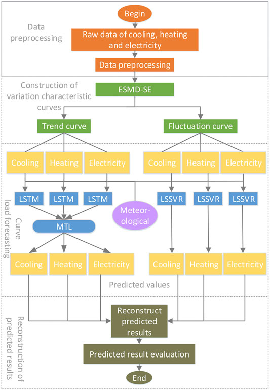
FIGURE 1. Flow chart of the MELF_MECVCC model.
ESMD-SE Method
ESMD method is an improvement made on the basis of EMD method. EMD is a data adaptive analysis method, which is suitable for the analysis of nonlinear and nonstationary signal sequences. It smooths complex signals and extracts IMFs and R0 parts with different characteristic scales or natural periods. However, the decomposed trend function is too rough, and the number of screening is difficult to determine. The obtained modal components include inherent modalities and abnormal events or include components of adjacent characteristic time scale. Therefore, EMD cannot effectively separate different modal components according to the characteristic time scale, resulting in “mode mixing.” ESMD replaces the outer envelope interpolation of EMD with internal pole symmetric interpolation. And it uses the principle of “least square” to optimize the remaining components to become the best “adaptive global moving average” for the entire data sequence. It can better reflect the changing trend of the data, so as to determine the optimal number of screening and solve the “mode mixing” problem in EMD.
ESMD has good adaptability and local variability based on the signal and has good processing ability for the nonstationary, nonlinear, and periodic random load time series. Therefore, we choose this method as the basis to decompose the load time series of each energy into different time scale modal components and trend residual according to frequency characteristics. The calculation steps of ESMD (Wang and Li, 2013) are as follows:
(1) Find the maximum value points and minimum value points of the sequence
(2) Use the (n+1) midpoints obtained in Step 1) to construct p interpolation lines, denoted as
(3) Repeat the above steps for sequence
(4) Repeat steps (1–3) for the sequence
(5) In the integer interval
In (2)
Among them,
SE is applied to measure the complexity of time series. From the perspective of the complexity of time series, it measures the probability of generating new patterns in the system and quantitatively describes the complexity and regularity of the system. The larger the SE, the more complex the time series, and the greater the probability so that the system will generate a new pattern. Conversely, the simpler the time series, the lower the probability.
Since the RIES load characteristic curves with strong fluctuation contingency, the original sequences of multienergy load time series are decomposed by ESMD. After a comprehensive analysis of SE data, the variation characteristic curves of multienergy can be reconstructed, including trend curve and fluctuation curve, and they are respectively modeled and predicted. As for the trend curve, its fluctuation period is longer and greatly affected by the long-term series. We choose the MTL-LSTM method for prediction. As for the fluctuation curve, the fluctuation frequency is relatively high, and the LSSVM method with better adaptability to the fluctuation sequence is applied for prediction.
MTL-LSTM Prediction Model
When dealing with nonlinear problems, the traditional machine learning method is to solve the problem by dividing the problem into several small, relatively independent subtasks, processing each subtask separately, and recombining them. Therefore, this method splits the correlation between each task under the same problem and loses a lot of useful information, so that the concept of MTL has come into being. MTL introduces the concept of induced migration mechanism to process all or some of the m tasks that are related but not exactly the same (Caruana, 1997; Nunes et al., 2019). It makes full use of the shared information contained in m tasks and trains these tasks in parallel to achieve the goal of improving the performance of each task. MTL can not only improve the learning efficiency and application performance of each task, but also greatly reduce the model scale. In this article, we use the hard parameter sharing mechanism in its parameter sharing mechanisms, as shown in Figure 2. Multiple tasks share one or more common hidden layers in the network while retaining the output layers related to the problem, thereby improving efficiency and reducing the risk of overfitting. For the MELF problem in RIES with many parameters and complex structure, its parameter characteristics and model structure are relatively simple, and its generalization ability is stronger.
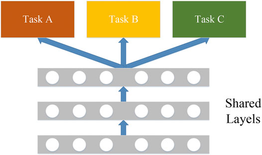
FIGURE 2. MTL of hard parameter sharing mechanism.
LSTM network is an improved RNN. Due to the “gradient disappearance” problem caused by the limited memory and storage space of RNN, LSTM inherits RNN’s good temporal correlation for sequential data problems and also introduces gate mechanism and memory units that make it perform well in representing historical information and future information and extracting the long distance dependence relation of elements in time series data. Therefore, LSTM has become a current popular RNN structure and can be used in many application scenarios.
Figure 3 shows the basic unit structure of the LSTM network, including forget gate, input gate, and output gate. The forgetting part of the state memory unit is composed of the forget gate input
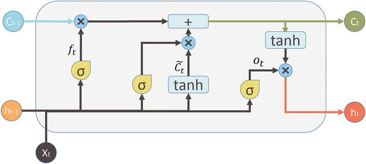
FIGURE 3. Basic unit structure of LSTM network.
Here,
LSSVR Prediction Model
LSSVR is a pattern recognition algorithm based on statistical learning theory, following the principle of structural risk minimization. It replaces the inequality constraints of SVR with equality constraints, transforms the quadratic programming problem into linear programming problem to solve, so as to reduce the computational complexity and improve the convergence speed (Suykens and Vandewalle, 1999). Compared with the neural network using heuristic method and having empirical components in its implementation, LSSVR has a more rigorous theoretical and mathematical foundation, does not have a local minimum, and has strong generalization performance. Since the time series of the fluctuation curve fluctuates greatly in frequency, and the long-term dependence on time is not obvious, LSSVR is more suitable for the prediction of fluctuation curve, and the prediction performance is better.
Here, we suppose the sample set
where
According to the above formula, the Lagrange function is constructed as
where
After calculating the Lagrange derivative of Formula (11), we can get
where
By substituting into the calculation and selecting the RBF function as the kernel function, the LSSVR prediction model is finally obtained as
Numerical Analysis
Data Source and Processing of Input Variables
The data set to verify the MELF_MECVCC algorithm in this study is taken from the actual data set UTA—the main campus of the University of Texas in Austin provided in literature (Powell et al., 2014). The data set covers an area of 1.6 million square meters and contains more than 160 buildings. The content of the data set includes hourly cooling, heating, electricity load data, and corresponding meteorology influence factor data like dry bulb temperature, wet bulb temperature, and relative humidity.
The training set time selected in this research is from 1:00 on September 10, 2011 to 24:00 on March 9, 2012, and the test set time is from 1:00 on March 10, 2012 to 24:00 on March 16, 2012. Suppose the current time step is
Construction of Variation Characteristic Curves and Explanation of Its Multienergy Coupling
tThe influence factors of multienergy in RIES have long-term and short-term characteristics. The long-term characteristics such as periodic changes on climate of regional characteristics and cultural customs make the loads have trend characteristic, and the short-term characteristics such as current weather changes and human life activities make the loads have fluctuation characteristic. The trend can effectively characterize the changing trend of the total load curve, and volatility can highlight load fluctuations caused by accidental factors. When performing MELF, considering the variation characteristics can not only effectively grasp the changing characteristics of multienergy sources and improve the accuracy of prediction, but also further explore the coupling information between energy sources under the variation characteristics and strengthen the learning of multienergy coupling characteristic. Therefore, the trend curve and fluctuation curve of each energy load time series are constructed by the ESMD-SE method. First, the load time series of the three energy sources are separately decomposed by ESMD to obtain IMFs and R0. Then, by comprehensively analyzing the SE of the original sequence and each component sequence, as shown in Table 1, we reconstruct the trend curve and fluctuation curve of each energy sequence.

TABLE 1. The SE of the original energy sequences and each component sequence.
It can be seen from Table 1 that the SE of the sequence
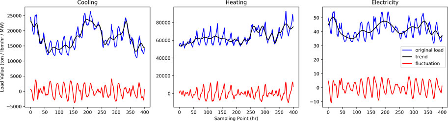
FIGURE 4. Original load curves and variation characteristic curves of cooling, heating, and electricity.
RIES’s multienergy sources have interactive responses and complementary features of generation, conversion, consumption, etc., which have strong coupling. Therefore, we consider the multienergy coupling of variation characteristic curves for MELF to enhance the coupling information sharing and learning. Here, the Pearson correlation coefficient is used to measure the multienergy coupling of the trend curve or the fluctuation curve. Pearson’s correlation coefficient is expressed as
In (15),
As shown in Table 2, in the trend curve part, the correlation coefficients between the load at historical moments

TABLE 2. Multienergy correlation coefficient of variation characteristic curves.
Experimental Evaluation Index
The prediction effect of the MELF_MECVCC model in this study is measured by the RMSE, the MAPE, and the RE as evaluation index. The formula of RMSE, MAPE, and RE is as follows:
In (16–18),
Comparison and Analysis of Forecast Results
In the experimental verification of the MELF-MECVCC model, the explanation is divided into two parts. The first part is to analyze and compare the predicted results of multiple models to verify the prediction accuracy and improvement advantages of the model proposed here. We select BPNN, OP-ELM as unused method comparison items and LSTM, LSSVR, ESMD-SE-LSTM-LSSVR as used method comparison items. The second part is to analyze and compare the decomposition algorithm in the construction of the variation characteristic curves. We select EMD and VMD as comparative verification. The methods and numbers of the selected comparison models are shown in Table 3.
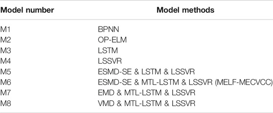
TABLE 3. The list of compared models.
Comparison and Analysis of Multiple Models
When testing and verifying the experiment, the MELF_MECVCC model as M6 is obtained by training the training set, and the model prediction effect is tested on the test set. The experimental data set and model acquisition steps of M1–M5 are the same as those of M6. Figure 5 is a comparison diagram of the actual load curves and the predicted load curves of the six models based on the cooling, heating, and electricity data in the test set. Figure 6 is a comparison diagram of the actual load curves and the predicted load curves based on the subsample sequence in the test set with a time span of one day.
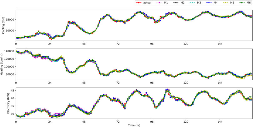
FIGURE 5. Actual load curves and predicted load curves of M1-M6 based on the test set.
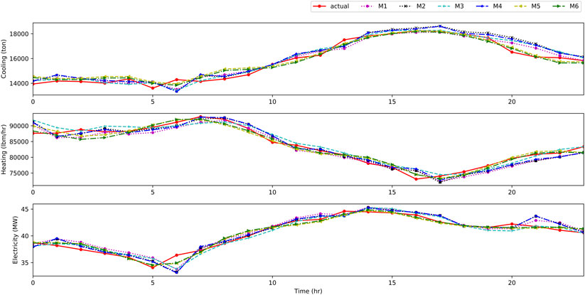
FIGURE 6. Actual load curves and predicted load curves of M1-M6 on March 13.
As shown in Figure 5, the six models all fit well with the actual load curves. Due to the relatively large amount of data, the subsequence samples in Figure 6 are used for illustration. Figure 6 gives the comparison between actual and predicted curves in the test set on March 13. M1 and M3 are relatively flat, so they cannot adapt to actual load curve fluctuations, while M2 and M4 have larger fluctuations. For example, at 7:00 (0 scale point of the abscissa in the figure represents 1:00), the predicted curves of M2 and M4 for electricity and cooling fluctuate greatly. But from an overall perspective, it is also obvious that LSSVR has good generalization characteristics for sequences with large fluctuations. It can be seen from the figure that the predicted values of M5 and M6 are closer to the actual load values of cooling, heating, and electricity, and when the actual loads fluctuate, the fitting effect of M1–M4 to the actual load curves is lagging compared to M5 or M6. M5 and M6 can improve the fitting effect of the predicted curve by considering the multienergy coupling of variation characteristic curves.
The three subgraphs in Figure 7 show the prediction errors of cooling, heating, and electricity based on M1-M6. For the prediction error evaluation indexes RMSE and MAPE, the prediction errors of M1-M6 from large to small are M1, M3 > M2, M4 > M5 > M6. Compared with M3 and M4, the MAPE of M5 is reduced by 25.94 and 20.24% for cooling, 27.75 and 14.81% for heating, and 24.14 and 6.38% for electricity. On the basis of M5 considering the multienergy coupling of variation characteristic curves, M6 introduces MTL method for the trend curve, and the MAPE of M6 is reduced by 4.06, 23.19, and 6.06%, respectively, for cooling, heating, and electricity, compared with M5. M6 makes full use of the sharing information and further improves the prediction accuracy. Among the six models, M6 has the smallest error value indicating the best fitting effect.
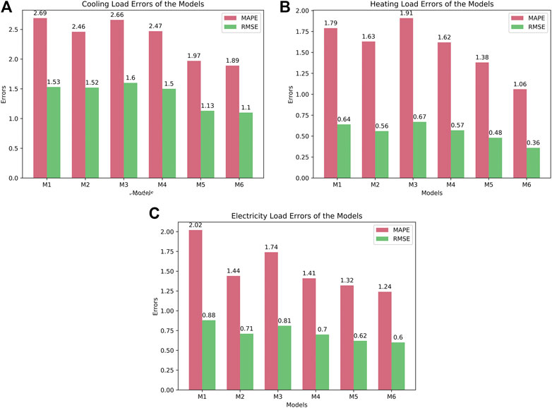
FIGURE 7. Model prediction errors of (A) cooling, (B) heating, and (C) electricity.
Figure 8 is a box diagram of the RE percentage distribution of cooling, heating, and electricity based on M1–M6. The REs of M5 and M6 are reduced compared with M1–M4, and the error distribution range of M5 and M6 is also significantly reduced. It shows that considering the multienergy coupling under the variation characteristics can reduce the RE of the prediction model. Among the six models, M6 has the smallest RE and fewer outliers, which highlights that the MELF_MECVCC model proposed in this article has a certain effect on the accuracy of MELF and has more research and application value.
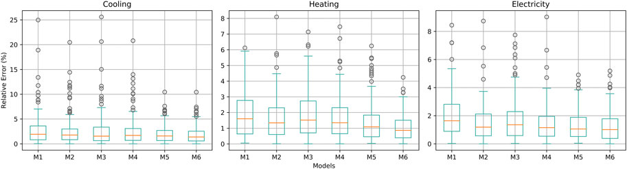
FIGURE 8. Model relative error distribution box diagram of cooling, heating, and electricity.
Comparison and Analysis of Decomposition Algorithms
On the basis of other algorithms remaining unchanged, the decomposition algorithm is changed to EMD and VMD. We denote their models as M7 and M8, respectively, and compare them with the proposed M6 whose decomposition algorithm is ESMD. Figure 9 is a comparison diagram of the actual load curves and the predicted load curves of M6, M7, and M8 based on the cooling, heating, and electricity data in the test set. Table 4 is the prediction errors of M6–M8 and the comparison of the error reduction relative to M3 and M4. Figure 10 shows the distribution curves of the RE percentage of M6–M8 for multienergy loads.
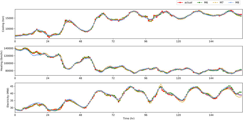
FIGURE 9. Actual load curves and predicted load curves of M6-M8 based on the test set.

TABLE 4. The errors of M6-M8 and their error reduction compared with reference M3 and M4.
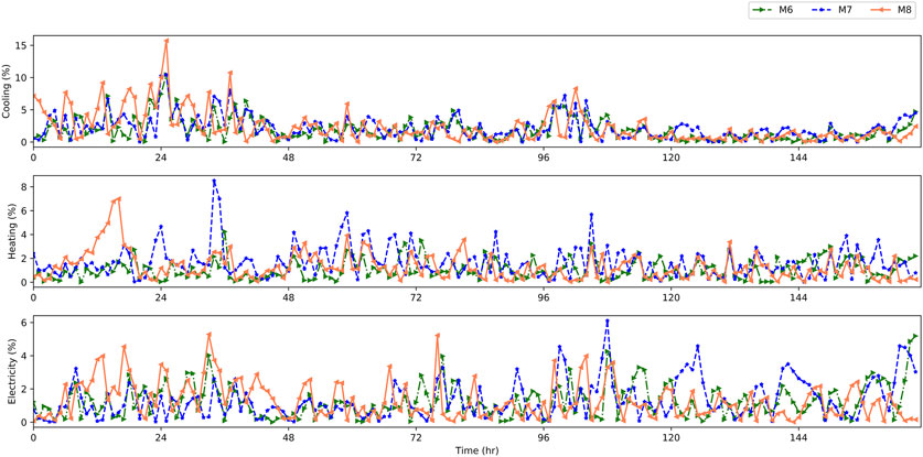
FIGURE 10. Model relative error distribution curves of cooling, heating, and electricity.
As shown in Figure 9, under the premise of considering the multienergy coupling of variation characteristic curves, the predicted load curves of M6–M8 all have a higher degree of fit to the actual load curves. However, the curves of M7 and M8 still have more outliers, and the degree of fit is worse than M6. In Table 4, the reductions of MAPE and RMSE of M6, M7, and M8 relative to M3 and M4 are compared respectively. For example, in line 2, column 3, the data 1.89 (28.95, 23.48) means that the MAPE of M6 is 1.89% and it is 28.95% less than that of M3 in cooling load forecasting calculated by (MAPEM3-MAPEM6)/MAPEM3, and it is 23.48% less than that of M4 in cooling load forecasting calculated by (MAPEM4-MAPEM6)/MAPEM4. Except that the heating RMSE of M7 does not decrease, the prediction errors of M6-M8 are significantly reduced compared with M3 and M4. Taking MAPE as an example, the cooling error is reduced by more than 15%, the electricity error is reduced by more than 20%, and the heating errors of M6 and M8 are both reduced by more than 30%, which further proves that considering the multienergy coupling of variation characteristic curves can deeply explore the coupling information elements in the context of physical information interconnection of the RIES and improve the accuracy of MELF. Moreover, M7 has a better effect on cooling and electricity load information processing, and M8 has better effect on heating and electricity load information processing, but M6 has better effect on the three kinds of energy load information mining and energy forecasting than M7 and M8, with the error reduction greater than 12, 17, and 3% for cooling, heating, and electricity, respectively.
According to Figure 10, the prediction RE distribution curves of the three models, M6 has a smaller error distribution range than M7 and M8, and its RE value is lower. In addition, the value and number of outlier points of M6 are significantly smaller than those of M7 and M8. Therefore, after comprehensively analyzing the performance of the decomposition algorithms for constructing the variation characteristic curves of cooling, heating, and electricity, we choose ESMD to better meet the accuracy requirement of the research.
Conclusion
In this research, the MELF_MECVCC combined model designed for RIES was investigated. The obtained results are as follows.
(1) The multienergy variation characteristic curves are decomposed and reconstructed through ESMD-SE, and the load variation features and energy coupling information are deeply excavated. Compared with EMD and VMD as the decomposition algorithm, the errors of the model proposed which uses ESMD are reduced by more than 12, 17, and 3% for cooling, heating, and electricity.
(2) This method considers the multienergy coupling of variation characteristic curves. According to the analysis of Pearson’s correlation coefficient, the closer to the current moment of prediction, the stronger the coupling between energy sources. Also, there is a very strong correlation between the loads of the trend curve and a moderate correlation between the loads of the fluctuation curve.
(3) Compared with BPNN, OP-ELM, LSTM, and LSSVR, the prediction results of the MELF_MECVCC model are reduced by more than 23, 34, and 12% respectively for cooling, heating, and electricity. This model has the highest prediction accuracy and the smallest distribution range of prediction errors. It can better fit the actual load curves and deeply explore the load temporal and spatial characteristics and energy interconnection coupling characteristics due to the variation characteristics of the energy sources.
In summary, the method proposed further improves the prediction accuracy of multienergy load forecasting and has certain research value and practical application value. Its predicted results can provide accurate data support for energy planning and dispatch and then ensure the safe and stable operation of the multienergy systems.
Data Availability Statement
The original contributions presented in the study are included in the article/Supplementary Material; further inquiries can be directed to the corresponding author.
Author Contributions
SW was involved in methodology, formal analysis, validation, writing: original draft review and editing, and visualization. KW contributed to conceptualization, software, investigation, and writing: original draft editing. QZ contributed to data curation, resources, and writing: review and editing. SW was involved in data curation and resources. LF and ZZ were involved in funding acquisition. GW was involved in project administration. All authors contributed to the article and approved the submitted version.
Funding
This work was supported by the Shandong Electric Power Company Science and Technology Project and the S&T Program of Hebei (20312102D).
Conflict of Interest
The authors declare that the research was conducted in the absence of any commercial or financial relationships that could be construed as a potential conflict of interest.
Supplementary Material
The Supplementary Material for this article can be found online at: https://www.frontiersin.org/articles/10.3389/fenrg.2021.635234/full#supplementary-material.
Glossary
ANFIS Adaptive neurofuzzy inference system
ANN Artificial neural network
ARMA Autoregressive moving average
BPNN Back propagation neural network
BSGP Bayesian spatiotemporal Gaussian process
DBN Deep belief network
DNN Deep neural network
ELM Extreme learning machine
EMD Empirical mode decomposition
ESMD Extreme-point symmetric mode decomposition
FOA Fruit fly optimization algorithm
IMF Intrinsic mode function
LSSVM Least square support vector machine
LSSVR Least square support vector regression
LSTM Long short-term memory network
>MAPE Mean absolute percentage error
MELF Multienergy load forecasting
MELF_MECVCC A MELF method for RIES considering multienergy coupling of variation characteristic curves (the model proposed)
MTL Multitask learning
OP-ELM Optimally pruned extreme learning machine
R0 Residual error
RE Relative error
RIES Regional integrated energy systems
RMSE Root mean square error
RNN Recursive neural network
SE Sample entropy
SVM Support vector machine
SVR Support vector regression
VAR Vector autoregressive
VMD Variational mode decomposition
XGBoost Extreme gradient boosting.
References
Chen, Y., Kloft, M., Yang, Y., Li, C., and Li, L. (2018). Mixed kernel based extreme learning machine for electric load forecasting. Neurocomputing 312, 90–106. doi:10.1016/j.neucom.2018.05.068
Chen, Z. Y., Liu, J. B., Li, C., Ji, X. H., Li, D. P., and Huang, Y. H. (2020). Ultra short-term power load forecasting based on combined LSTM-XGBoost model. Power Syst. Tech. 44 (2), 614–620. doi:10.13335/j.1000-3673.pst.2019.1566
Dudek, G. (2016). Pattern-based local linear regression models for short-term load forecasting. Electric Power Syst. Res. 130, 139–147. doi:10.1016/j.epsr.2015.09.001
Dung, N. T., and Phuong, N. T. (2019). Short-term electric load forecasting using standardized load profile (SLP) and support vector regression (SVR). Eng. Technol. Appl. Sci. Res. 9 (4), 4548–4553. doi:10.48084/etasr.2929
Fard, A. K., and Akbari-Zadeh, M.-R. (2014). A hybrid method based on wavelet, ANN and ARIMA model for short-term load forecasting. J. Exp. Theor. Artif. Intelligence 26 (2), 167–182. doi:10.1080/0952813x.2013.813976
Gilanifar, M., Wang, H., Sriram, L. M. K., Ozguven, E. E., and Arghandeh, R. (2020). Multitask Bayesian spatiotemporal Gaussian processes for short-term load forecasting. IEEE Trans. Ind. Electron. 67 (6), 5132–5143. doi:10.1109/tie.2019.2928275
Hochreiter, S., and Schmidhuber, J. (1997). Long short-term memory. Neural Comput. 9 (8), 1735–1780. doi:10.1162/neco.1997.9.8.1735
Jamaaluddin, U., Robandi, I., and Anshory, I. (2019). A very short-term load forecasting in time of peak loads using interval type-2 fuzzy inference system: a case study on java bali electrical system. J. Eng. Sci. Tech. 14 (1), 464–478. doi:10.1088/1757-899X/403/1/012070
Jiao, R., Zhang, T., Jiang, Y., and He, H. (2018). Short-term non-residential load forecasting based on multiple sequences LSTM recurrent neural network. IEEE Access 6, 59438–59448. doi:10.1109/access.2018.2873712
Khorram-Nia, R., and Karimi-Khorami, S. (2015). Short term load forecasting in power systems using a hybrid approach based on SVR technique. Ifs 29 (1), 119–125. doi:10.3233/ifs-141575
Kong, W., Dong, Z. Y., Jia, Y., Hill, D. J., Xu, Y., and Zhang, Y. (2017). Short-term residential load forecasting based on LSTM recurrent neural network. IEEE Trans. Smart Grid. 10 (1), 841–851. 10.1109/TSG.2017.2753802.
Li, M.-W., Geng, J., Hong, W.-C., and Zhang, Y. (2018a). Hybridizing chaotic and quantum mechanisms and fruit fly optimization algorithm with least squares support vector regression model in electric load forecasting. Energies 11 (9), 2226. doi:10.3390/en11092226
Li, Y. J., Yuan, X. L., Xu, J. Y., Chen, Z., and Li, H. M. (2018b). Medium-term forecasting of cold, electric and gas load in multienergy system based on VAR model,” in 2018 13th IEEE conference on industrial electronics and applications (ICIEA). Wuhan, China, 31 May–2 June, 2018. (Piscataway, NJ: IEEE).
Liu, D., Wang, L., Qin, G., and Liu, M. (2020). Power load demand forecasting model and method based on multienergy coupling. Appl. Sci. 10 (2), 584. doi:10.3390/app10020584
Liu, M., Shi, Y., and Fang, F. (2015). Load forecasting and operation strategy design for CCHP systems using forecasted loads. IEEE Trans. Control. Syst. Tech. 23 (5), 1672–1684. 10.1109/TCST.2014.2381157.
Ma, T., Wang, F., Wang, J., Yao, Y., and Chen, X. (2017). A combined model based on seasonal autoregressive integrated moving average and modified particle swarm optimization algorithm for electrical load forecasting. Ifs 32 (5), 3447–3459. doi:10.3233/jifs-169283
Mi, J., Fan, L., Duan, X., and Qiu, Y. (2018). Short-term power load forecasting method based on improved exponential smoothing grey model. Math. Probl. Eng. 2018, 1–11. doi:10.1155/2018/3894723
Motepe, S., Hasan, A. N., and Stopforth, R. (2019). Improving load forecasting process for a power distribution network using hybrid ai and deep learning algorithms. IEEE Access 7, 1. doi:10.1109/access.2019.2923796
Nunes, M., Gerding, E., McGroarty, F., and Niranjan, M. (2019). A comparison of multitask and single task learning with artificial neural networks for yield curve forecasting. Expert Syst. Appl. 119, 362–375. doi:10.1016/j.eswa.2018.11.012
Ouyang, T., He, Y., Li, H., Sun, Z., and Baek, S. (2019). Modeling and forecasting short-term power load with copula model and deep belief network. IEEE Trans. Emerg. Top. Comput. Intell. 3 (2), 127–136. doi:10.1109/tetci.2018.2880511
Powell, K. M., Sriprasad, A., Cole, W. J., and Edgar, T. F. (2014). Heating, cooling, and electrical load forecasting for a large-scale district energy system. Energy 74, 877–885. doi:10.1016/j.energy.2014.07.064
Ryu, S., Noh, J., and Kim, H. (2017). “Deep neural network based demand side short term load forecasting,” in 2016 IEEE International Conference On Smart Grid Communications (Smartgridcomm), Sydney, NSW, Australia, November 6–9, 2016. (Piscataway, NJ: IEEE).
Shi, J. Q., Tan, T., Guo, J., Liu, Y., and Zhang, J, H. (2018). Multi-task learning based on deep architecture for various types of load forecasting in regional energy system integration. Power Syst. Tech. 42 (3), 698–706. doi:10.1016/j.ijepes.2020.106583
Singh, P., and Dwivedi, P. (2019). A novel hybrid model based on neural network and multi-objective optimization for effective load forecast. Energy 182, 606–622. doi:10.1016/j.energy.2019.06.075
Suykens, J. A. K., and Vandewalle, J. (1999). Least squares support vector machine classifiers. Neural Process. Lett. 9 (3), 293–300. doi:10.1023/a:1018628609742
Wang, J.-L., and Li, Z.-J. (2013). Extreme-point symmetric mode decomposition method for data analysis. Adv. Adapt. Data Anal. 5 (3), 1350015. doi:10.1142/s1793536913500155
Yuan, K., Li, J. R., Song, Y., Mu, Y. F., Sun, C. B., and Xu, Y. (2019). Review and prospect of comprehensive evaluation technology of regional energy internet. Auto. Electric Power Syst. 43 (14), 41–52. doi:10.7500/AEPS20181129009
Zhang, G., Liu, H., Li, P., Li, M., He, Q., and Jinwang, H., Prediction based on hybrid model of vmd-mrmr-bpnn-lssvm. Complexity, 2020 (4), 1–20. doi:10.1155/2020/6940786
Zhang, H., Yuan, J., and Chen, L. (2017). Short-term load forecasting using EMD-LSTM neural networks with a Xgboost algorithm for feature importance evaluation. Energies 10 (8), 1168. doi:10.3390/en10081168
Zhong, W., Zhuang, Y., Sun, J., and Gu, J. (2019). Load forecasting for cloud computing based on wavelet support vector machine. Ijhpcn 14 (3), 315–324. doi:10.1504/ijhpcn.2019.102131
Zhou, J., Yu, X., and Jin, B. (2018). Short-term wind power forecasting: a new hybrid model combined extreme-point symmetric mode decomposition, extreme learning machine and particle swarm optimization. Sustainability 10 (9), 3202. doi:10.3390/su10093202
Keywords: multienergy load forecasting, integrated energy systems, multienergy coupling, mode decomposition, long short-term memory
Citation: Wang S, Wu K, Zhao Q, Wang S, Feng L, Zheng Z and Wang G (2021) Multienergy Load Forecasting for Regional Integrated Energy Systems Considering Multienergy Coupling of Variation Characteristic Curves. Front. Energy Res. 9:635234. doi: 10.3389/fenrg.2021.635234
Received: 30 November 2020; Accepted: 29 January 2021;
Published: 08 April 2021.
Edited by:
Vahid Vahidinasab, Newcastle University, United KingdomReviewed by:
Yusen He, The University of Iowa, United StatesGiorgio Graditi, Energy and Sustainable Economic Development (ENEA), Italy
Copyright © 2021 Wang, Wu, Zhao, Wang, Feng, Zheng and Wang. This is an open-access article distributed under the terms of the Creative Commons Attribution License (CC BY). The use, distribution or reproduction in other forums is permitted, provided the original author(s) and the copyright owner(s) are credited and that the original publication in this journal is cited, in accordance with accepted academic practice. No use, distribution or reproduction is permitted which does not comply with these terms.
*Correspondence: Qianyu Zhao, emhhb3FpYW55dUB0anUuZWR1LmNu