Optimal Balancing of Wind Parks with Virtual Power Plants

In this paper, we explore the optimization of virtual power plants (VPP), consisting of a portfolio of biogas power plants and a battery whose goal is to balance a wind park while maximizing their revenues. We operate under price and wind production uncertainty and in order to handle it, methods of machine learning are employed. For price modeling, we take into account the latest trends in the field and the most up-to-date events affecting the day-ahead and intra-day prices. The performance of our price models is demonstrated by both statistical methods and improvements in the profits of the virtual power plant. Optimization methods will take price and imbalance forecasts as input and conduct parallelization, decomposition, and splitting methods in order to handle sufficiently large numbers of assets in a VPP. The main focus is on the speed of computing optimal solutions of large-scale mixed-integer linear programming problems, and the best speed-up is in two orders of magnitude enabled by our method which we called Gradual Increase.

1 Introduction

The optimization of virtual power plants (VPP) is of crucial importance as it enables the more efficient incorporation of distributed energy resources (DER) into the grid and thereby contributes to the achievement of goals associated with ecology. Solar and wind energy sources have a degree of uncertainty and require constant balancing. Therefore, from an ecological point of view, it is desirable that the balancing is carried out by flexible energy sources operating on a renewable fuel. In our case studies, we consider the balancing of wind parks by means of pools of biogas (renewable fuel) power plants and pools of batteries and propose ways to accelerate calculations by means of mathematical methods of decomposition and splitting, leveraging the special structure of problems, parallelization, and the brute force power of optimization solvers. In our VPP, state-of-the-art commercial wind forecasts are used in order to nominate the amounts of energy that our wind turbines are able to produce, and the goal of the flexible assets is to handle the aggregate imbalances in both directions: biogas power plants can balance only deficiencies while batteries can also balance surpluses.

The goal of the biogas power plants and batteries is to maximize their revenues from selling electricity on the day-ahead and intra-day markets while providing balancing to the pool of intermittent assets. One important research component within the optimization of VPPs is the method known as Alternating Direction Method of Multipliers (ADMM), which is a technique based on replacing the solution of a large-scale optimization problem with an iterative procedure involving solutions of a large number of small subproblems. (Chen and Li, 2018; Munsing et al., 2017). A special facet of this method known as Proximal Jacobian ADMM is proven to $o\left(\frac{1}{k}\right)$-converge for linear programming problems and to be amenable to parallelization (Deng et al., 2017). This algorithm will also be used in our research. In this study, this method for optimizing large pools of power plants where we deal with integer variables is applied.

Before taking up the main topic of this paper, we mention relevant research in the field of optimizing Virtual Power Plants. The scope of optimization methods for managing virtual power plants is relatively broad and incorporates approaches such as linear programming, mixed-integer linear programming, methods based on dynamic programming, multistage bilevel algorithms, evolutionary algorithms, etc. (Podder et al., 2020). In Müller et al. (2015), a virtual power plant is optimized by linear programming methods and the polytope of the constraints is approximated with a zonotope—a structure closed under Minkowski addition. This provides an inner approximation of the constraints and this structure requires less memory than the original problem hence helping with the curse of dimensionality and providing a feasible (although suboptimal) solution. A zonotopic approximation is bottom-up: constraints associated with each asset in a VPP are approximated with a zonotope and then summed up with the Minkowski addition yielding the zonotope of the entire VPP. This enables us to efficiently add new assets into the pool (polynomial complexity) provided that the constraints associated with each asset are linear. In Tan et al. (2018), the authors explore the management of virtual power plants and their alliances involving wind and solar parks. They propose a model involving the separate operation of assets but joint scheduling of them. Their model is based on Shapley value theory for profit distribution, and it is applied to case studies in China. In Chen and Li (2018), the authors provide ADMM-based dispatch techniques for virtual power plants where they propose their own algorithm in which each DER communicates information only with its neighbors in order to collectively find the global optimal solution. The algorithm is fully distributed, it does not require a central controller, and the proof of its convergence is presented. In Munsing et al. (2017), the authors propose the algorithm of the implementation of ADMM within the blockchain while conducting the aggregation by means of a smart contract which can be used for any ADMM-based algorithm. The main point is that the aggregation relates to elementary operations with matrices and vectors, i.e. the operations that can be implemented within ADMM in a matter of milliseconds. In Wytock (2016), Moehle et al. (2019), the authors provide the management of virtual power plants where gas-fired power plants balance a wind park and in the wind forecast methods, they use spatial correlations. In Moehle et al. (2019), the authors propose a technique called Robust Model Predictive Control which is also employed in the management of the VPP in this paper. In Nguyen et al. (2020), Duong et al. (2020), the authors utilize metaheuristic algorithms such as Stochastic Fractal Search for the optimal reactive power flow of 118-bus systems. In Filippo et al. (2017), Pandžić et al. (2013a), Pandžić et al. (2013b), Mashhour and Moghaddas-Tafreshi (2011), the authors propose the management of virtual power plants by mixed-integer optimization algorithms (Elkamel et al., 2021). explores price-based unit commitment. Enumeration of all optimization methods would exceed the scope of this publication, but we can refer the reader to (Podder et al., 2020), which provides a thorough categorization of these methods in the field and to (Ackooij et al., 2018), which provides a literature survey of unit commitment methods. According to (DCbrain, 2020), it is crucial to incorporate biogas power plants into the grid.

There are studies where virtual power plants include biogas power plants, e.g. in Candra et al. (2018), Vicentin et al. (2019), Wegener et al. (2021). In Ziegler et al. (2018) and Egieya et al. (2020), the virtual power plant includes biogas power plants and the operation of this entity involves solving a large-scale mixed-integer linear programming problem (MILP). We also solve large-scale MILP problems and the focus is on balancing of wind parks, but it can easily be shown that the logic of the presented algorithms can be translated to broader classes of intermittent sources (Graabak and Korpås, 2016).

The main contribution of this research is the method called Gradual Increase which is a heuristic that was applied in the optimization of pools of assets. This is a decomposition technique based on the operations with sub-pools of assets and with warm starts. The utilization of this method enabled us to significantly accelerate the calculations and in the best case, it was up to two orders of magnitude. In general, this method demonstrates significant improvements in revenues compared to the brute force approach when limited by times typical for real-time applications, which is shown in Section 7. The Gradual Increase method is compared with other methods such as Proximal Jacobian ADMM in terms of average calculation time. We also demonstrate further improvements in average calculation times when a hybrid of Gradual Increase and Partial Integrality is employed.

The method of Gradual Increase is tested within real-time optimization settings: an MILP problem is solved every 24 h taking into account the state of the system (storage levels and states of the units) and the forecasts of prices and imbalances. The forecasts and the system’s states are updated every 24 h and apart from the optimization, we implement financial settlements associated with optimization decisions. These settings are formulated by means of MPC and RMPC where the latter enables us to incorporate randomness into the model (Moehle et al., 2019). Large-scale MILP problems with four up to hundreds of assets are solved in the deterministic environment (MPC) using only commercial price forecasts; problems with the three assets are solved in two environments: MPC and RMPC, and three more forecasting methods are employed there.

This paper has the following structure: the optimization problem is described in Section 2. Our method called Gradual Increase is described in Section 3. Section 4 describes our implementation of Model Predictive Control and Robust Model Predictive Control. Besides, this section provides additional methods for accelerating the solution of our optimization problems. The methods of machine learning applied for modeling and forecasting prices are mentioned in Section 5. Section 6 provides the details of the optimization that are worth mentioning according to the authors. Tables with results are provided in Section 7, and then we move to the conclusions.

2 Problem Description

In this section, we firstly describe the assets that we optimize and then formulate the optimization problem.

2.1 Assets That we Optimize

We have a portfolio of two biogas power plants and a battery, and their goal is to balance the production of wind parks located in 8 regions of Germany: the power plants and the battery are also located in Germany. This functions as follows: the operators of the wind assets forecast how much energy their assets will produce. Wind production is uncertain because it is weather dependent, therefore balancing such assets is of utmost importance. And it is the goal of the pool of biogas power plants and batteries to handle the aggregate imbalance. The names of neither biogas power plants nor batteries nor wind parks can be disclosed for confidentiality reasons. We have detailed data for two biogas power plants and one battery. The turbines within the biogas power plants have no classical timing constraints except for the condition that the maximum number of switches per year is limited to a predefined number. When exploring the speed of our algorithms, timing constraints are imposed because they are typical for the turbines, and the assets within the pool are replicated in order to explore how the increasing number of assets affects the speed of the calculations: when replicating assets, we predefine the number of assets in the pool and randomly assign the storage capacities, gas inflows, maximum and minimum productions of the turbines and minimum on and off times for the turbines within biogas power plants (timing constraints). In replicating, the wind park increases proportionally to the increase in flexible assets. This enables us to apply the proposed algorithms for a broader scope of asset types. We operate on the German market EEX (day-ahead and intra-day) and use the price forecasts as objective value coefficients. The imbalance is modeled by means of autoregressive models. In our biogas power plants, the processes of fertilization and electricity production are separated. We are guaranteed to obtain fixed amounts F_k (see Table 1) of biogas (measured in MWh) every 15 min and we concentrate only on electricity production. In this study, biogas power plants with heating rods have not been considered, but this is considered as a subject for further research. More details about our biogas power plants can be found in Appendix.

TABLE 1

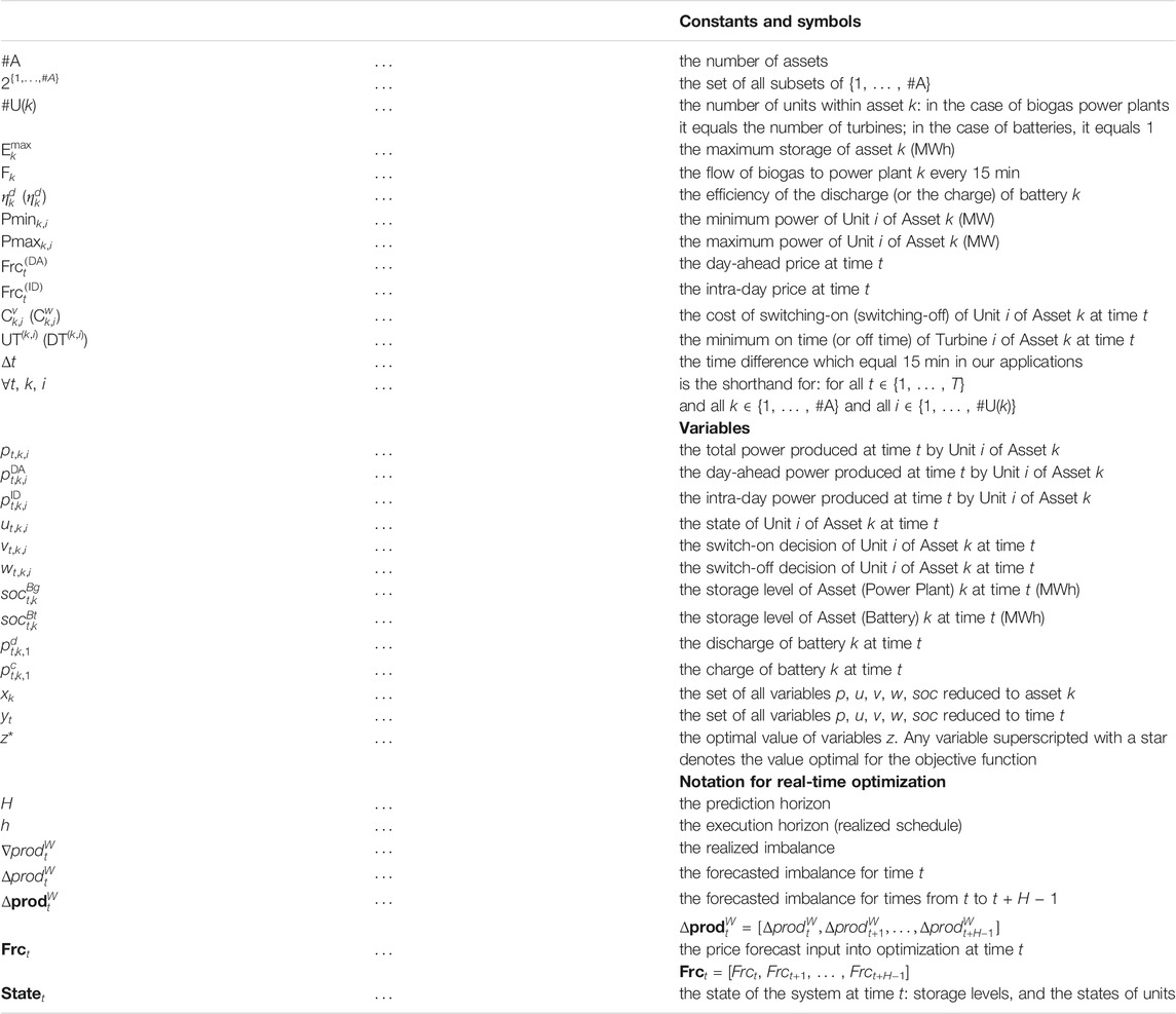
TABLE 1. Nomenclature.

2.2 The Objective

The objective is to maximize the revenues of pools of biogas power plants and batteries while balancing the wind park and taking technical constraints into account. The technical constraints of the turbines are their maximum and minimum production per period and the timing constraints. Following the notation from Table 1, the objective to be maximized is defined as follows:

$\sum _{t=1}^T\sum _{k=1}^{\mathrm{\#}\mathrm{A}}\sum _{i=1}^{\mathrm{\#}\mathrm{U}\left(k\right)}\left({\mathrm{F}\mathrm{r}\mathrm{c}}_t^{\left(\mathrm{D}\mathrm{A}\right)}{p}_{t,k,i}^{\text{DA}}+{\mathrm{F}\mathrm{r}\mathrm{c}}_t^{\left(\mathrm{I}\mathrm{D}\right)}{p}_{t,k,i}^{\text{ID}}-{\mathrm{C}}_{k,i}^v{v}_{t,k,i}-{\mathrm{C}}_{k,i}^w{w}_{t,k,i}\right),(1)$

which implies that we optimize our revenue from the sale of energy on the market penalizing every switch-on and -off with costs ${\mathrm{C}}_{k,i}^v$ and ${\mathrm{C}}_{k,i}^w$, where k denotes the index of an asset and i is the index of a turbine. In the case of a battery, these costs are zero. The constant T denotes the prediction horizon that we use for the optimization and ${\mathrm{F}\mathrm{r}\mathrm{c}}_t^{(\mathrm{D}\mathrm{A})}$, ${\mathrm{F}\mathrm{r}\mathrm{c}}_t^{(\mathrm{I}\mathrm{D})}$ are the forecasts of day-ahead and intra-day prices, respectively.

2.3 Constraints for Turbines

In this subsection, all of the constraints associated with biogas power plants are described. 3bin formulation is employed (Morales-Espana et al., 2015), and all u, v, and w variables (Table 1) are binary, i.e.

$u_{t,k,i},v_{t,k,i},w_{t,k,i}\in \left\{\mathrm{0,1}\right\}\forall i,k,t.(2)$

2.3.1 Power Constraints

There are two basic values for every turbine: Pmin_k,i > 0 and Pmax_k,i > Pmin_k,i ∀k, i which implies that it can either do nothing or produce within the interval [Pmin_k,i, Pmax_k,i], i.e.

$p_{t,k,i}\in \left\{0\right\}\cup \left[{\mathrm{P}\mathrm{m}\mathrm{i}\mathrm{n}}_{k,i},{\mathrm{P}\mathrm{m}\mathrm{a}\mathrm{x}}_{k,i}\right]\forall t,k,i.(3)$

These constraints can be written using the u_t,k,i variables which equal 1 if at time t the i-th turbine of Asset k is on and it is 0 otherwise:

$p_{t,k,i}-{\mathrm{P}\mathrm{m}\mathrm{i}\mathrm{n}}_{k,i}{u}_{t,k,i}\ge 0,{\mathrm{P}\mathrm{m}\mathrm{a}\mathrm{x}}_{k,i}{u}_{t,k,i}-p_{t,k,i}\ge 0\forall i,k,t.(4)$

The power produced can be decomposed to two components: the power used for the Day-Ahead market and the power used for the Intra-Day market, i.e.

$p_{t,k,i}=p_{t,k,i}^{\text{ID}}+p_{t,k,i}^{\text{DA}}\forall i,k,t.(5)$

2.3.2 The Storage Constraints

Every biogas power plant k has its own storage and a constant flow of gas F_k (expressed in MWh) into it. The new storage level is equal to the old level added by F_k and subtracted by the aggregate energy produced by all turbines within Asset k during one period:

$so{c}_{t,k}^{Bg}=so{c}_{t-1,k}^{Bg}+{\mathrm{F}}_k-\sum _{i=1}^{\mathrm{\#}\mathrm{U}(\mathrm{k})}{p}_{t,k,i}\mathrm{\Delta }t\forall t,k,(6)$

and the box constraints:

$so{c}_{t,k}^{Bg}\in \left[0,{\mathrm{E}}_k^{\max }\right]\forall t,k.(7)$

2.4 The Timing Constraints

The on and off decisions for the turbines are conducted via binary switch-on (v) and binary switch-off (w) variables as follows (Morales-Espana et al., 2015):

$u_{t,k,i}-u_{t-1,k,i}=v_{t,k,i}-w_{t,k,i}\forall t,k,i.(8)$

If at time t a turbine i of asset k is on or off, it has to be on or off for at least UT^(k,i) and DT^(k,i) periods, respectively, which is expressed as follows:

$\sum _{j=t-{\mathrm{U}\mathrm{T}}^{\left(k,i\right)}+1}^t{v}_{j,k,i}\le u_{t,k,i}\text{\hspace{0.17em}and\hspace{0.17em}}\sum _{j=t-{\mathrm{D}\mathrm{T}}^{\left(k,i\right)}+1}^t{w}_{j,k,i}\le 1-u_{t,k,i}\forall t,k,i.(9)$

2.5 Timing Constraints Tuning

We have light requirements on our turbines from the biogas power plants that we explore: maximum number of switch-ons per year. These conditions can be handled by imposing penalties for switch-ons and switch-offs. On the other, hand there are, generally, turbines with strict timing constraints therefore in our exploration of the speed of the decomposition algorithms, timing constraints are intentionally imposed in order to broaden the scope of applications of our algorithms.

2.6 The Constraints for Batteries

This subsection shows all the constraints associated with batteries:

2.6.1 Power Constraints

Every battery in our pool has the following power constraints:

${\mathrm{P}\mathrm{m}\mathrm{a}\mathrm{x}}_{k,1}{u}_{t,k,1}-p_{t,k,1}^{\text{d}}\ge 0\forall t,k,(10)$

${\mathrm{P}\mathrm{m}\mathrm{a}\mathrm{x}}_{k,1}\left(1-u_{t,k,1}\right)-p_{t,k,1}^{\text{c}}\ge 0\forall t,k,(11)$

$p_{t,k,1}^{\text{c}}-{\mathrm{P}\mathrm{m}\mathrm{i}\mathrm{n}}_{k,1}{w}_{t,k,1}\ge 0\forall t,k,(12)$

$p_{t,k,1}^{\text{d}}-{\mathrm{P}\mathrm{m}\mathrm{i}\mathrm{n}}_{k,1}{v}_{t,k,1}\ge 0\forall t,k.(13)$

These constraints ensure that we cannot charge and discharge at the same time (Alqunun et al., 2020).

2.6.2 Storage Constraints

The update of the storage level and the state of charge is conducted as follows:

$so{c}_{t+\mathrm{\Delta }t,k}^{Bt}=so{c}_{t,k}^{Bt}+\mathrm{\Delta }t\cdot {\eta }_k^c\cdot p_{t,k,1}^{\text{c}}-\frac{\mathrm{\Delta }t\cdot p_{t,k,1}^{\text{d}}}{{\eta }_k^d}\forall t,k,(14)$

and the power is constant in the interval [t, t + Δt].

2.6.3 Tightening Constraints

$v_{t,k,1}\le u_{t,k,1}\text{\hspace{0.17em}and\hspace{0.17em}}{w}_{t,k,1}\le 1-u_{t,k,1}\forall t,k,(15)$

and for all t we have box constraints:

$so{c}_{t,k}^{Bt}\in \left[0,{\mathrm{E}}_k^{\max }\right]\forall t,k.(16)$

2.6.4 Switches of the Batteries

The on and off decisions for the batteries are conducted via binary switch-on (v) and binary switch-off (w) variables as follows:

$u_{t,k,i}-u_{t-1,k,i}=v_{t,k,i}-w_{t,k,i}\forall t,k.(17)$

2.6.5 Components in the Objective Value

We define the variables p_t,k,1 as follows:

$p_{t,k,1}=p_{t,k,1}^{\text{d}}-p_{t,k,1}^{\text{c}}\forall t,k,(18)$

which is included in the objective (1).

2.7 The Coupling Constraints

The coupling constraint is a task that all flexible assets have to fulfill. This is given by the imbalance ${\mathcal{B}}_t\forall t$ between the realized and forecasted production of the intermittent sources.

$\sum _{k=1}^{\mathrm{\#}\mathrm{A}}\sum _{i=1}^{\mathrm{\#}\mathrm{U}\left(k\right)}{p}_{t,k,i}^{\text{ID}}={\mathcal{B}}_t,\forall t.(19)$

Note that the right-hand side of Eq. 19 is the input we have to estimate. This boils down to estimating the imbalance which is a challenging task. In this study we approach the imbalance by means of two methods:

1. Taking the historical imbalance: perfect foresight. We will use it as a benchmark. This will be the upper bound to the problem.

2. Fitting the imbalance with ARMA processes and using simulations.

2.8 The Optimization Problem Formulation

Summarizing the aforementioned constraints and objectives, we can formulate the optimization problem with the forecast parameters: Frc^(DA), Frc^(ID) and $\mathcal{B}$ as follows:

$\begin{array}{lll}\hfill \mathrm{m}\mathrm{a}\mathrm{x}\mathrm{i}\mathrm{m}\mathrm{i}\mathrm{z}\mathrm{e}& \sum _{t=1}^T\sum _{k=1}^{\mathrm{\#}\mathrm{A}}\sum _{i=1}^{\mathrm{\#}\mathrm{U}\left(k\right)}\left({\mathrm{F}\mathrm{r}\mathrm{c}}_t^{\left(\mathrm{D}\mathrm{A}\right)}{p}_{t,k,i}^{\text{DA}}+{\mathrm{F}\mathrm{r}\mathrm{c}}_t^{\left(\mathrm{I}\mathrm{D}\right)}{p}_{t,k,i}^{\text{ID}}-{\mathrm{C}}_{k,i}^v{v}_{t,k,i}-{\mathrm{C}}_{k,i}^w{w}_{t,k,i}\right)\hfill & \hfill \\ \hfill \mathrm{s}.\mathrm{t}.& \left(2\right)-\left(19\right)\hfill & \hfill \end{array}$

which we denote as follows: $\mathrm{V}\mathrm{P}\mathrm{P}({\mathrm{F}\mathrm{r}\mathrm{c}}^{(\mathrm{D}\mathrm{A})},{\mathrm{F}\mathrm{r}\mathrm{c}}^{(\mathrm{I}\mathrm{D})},\mathcal{B})$.

For the problem $\mathrm{V}\mathrm{P}\mathrm{P}({\mathrm{F}\mathrm{r}\mathrm{c}}^{(\mathrm{D}\mathrm{A})},{\mathrm{F}\mathrm{r}\mathrm{c}}^{(\mathrm{I}\mathrm{D})},\mathcal{B})$, we define the additional notation:

1. ${\mathrm{V}\mathrm{P}\mathrm{P}}_x({\mathrm{F}\mathrm{r}\mathrm{c}}^{(\mathrm{D}\mathrm{A})},{\mathrm{F}\mathrm{r}\mathrm{c}}^{(\mathrm{I}\mathrm{D})},\mathcal{B})$ is the optimal solutions of the problem, i.e.:

${\mathrm{V}\mathrm{P}\mathrm{P}}_x\left({\mathrm{F}\mathrm{r}\mathrm{c}}^{\left(\mathrm{D}\mathrm{A}\right)},{\mathrm{F}\mathrm{r}\mathrm{c}}^{\left(\mathrm{I}\mathrm{D}\right)},\mathcal{B}\right)=\left(p^{\mathrm{DA}\ast },p^{\mathrm{ID}\ast },p^{\ast },p^{c\ast },p^{d\ast },u^{\ast },v^{\ast },w^{\ast },so{c}^{\ast }\right)$

2. ${\mathrm{V}\mathrm{P}\mathrm{P}}_r({\mathrm{S}\mathrm{p}\mathrm{t}}^{(\mathrm{D}\mathrm{A})},{\mathrm{S}\mathrm{p}\mathrm{t}}^{(\mathrm{I}\mathrm{D})},\mathcal{B})$ is the realized value of the problem, i.e.

${\mathbf{V}\mathbf{P}\mathbf{P}}_r\left({\mathbf{S}\mathbf{p}\mathbf{t}}^{\left(\mathrm{D}\mathrm{A}\right)},{\mathbf{S}\mathbf{p}\mathbf{t}}^{\left(\mathrm{I}\mathrm{D}\right)},\mathcal{B}\right)=\sum _{t=1}^T\sum _{k=1}^{\mathrm{\#}\mathrm{A}}\sum _{i=1}^{\mathrm{\#}\mathrm{U}\left(k\right)}\left({\mathrm{S}\mathrm{p}\mathrm{t}}_t^{\left(\mathrm{D}\mathrm{A}\right)}{\mathit{p}}_{t,k,i}^{\text{DA}\ast }+{\mathrm{S}\mathrm{p}\mathrm{t}}_t^{\left(\mathrm{I}\mathrm{D}\right)}{\mathit{p}}_{t,k,i}^{\text{ID}*}-{\mathrm{C}}_{k,i}^v{v}_{t,k,i}^{\ast }-{\mathrm{C}}_{k,i}^w{w}_{t,k,i}^{\ast }\right)$

3. ${\mathrm{V}\mathrm{P}\mathrm{P}}_{rv}({\mathrm{F}\mathrm{r}\mathrm{c}}^{(\mathrm{D}\mathrm{A})},{\mathrm{F}\mathrm{r}\mathrm{c}}^{(\mathrm{I}\mathrm{D})},\mathcal{B})$ is the revenue yielded from ${\mathrm{V}\mathrm{P}\mathrm{P}}_x({\mathrm{F}\mathrm{r}\mathrm{c}}^{(\mathrm{D}\mathrm{A})},{\mathrm{F}\mathrm{r}\mathrm{c}}^{(\mathrm{I}\mathrm{D})},\mathcal{B})$, i.e.

${\mathrm{V}\mathrm{P}\mathrm{P}}_{rv}\left({\mathrm{F}\mathrm{r}\mathrm{c}}^{\left(\mathrm{D}\mathrm{A}\right)},{\mathrm{F}\mathrm{r}\mathrm{c}}^{\left(\mathrm{I}\mathrm{D}\right)},\mathcal{B}\right)=\sum _{t=1}^T\sum _{k=1}^{\mathrm{\#}\mathrm{A}}\sum _{i=1}^{\mathrm{\#}\mathrm{U}\left(k\right)}\left({\mathrm{F}\mathrm{r}\mathrm{c}}_t^{\left(\mathrm{D}\mathrm{A}\right)}{p}_{t,k,i}^{\text{DA}\ast }+{\mathrm{F}\mathrm{r}\mathrm{c}}_t^{\left(\mathrm{I}\mathrm{D}\right)}{p}_{t,k,i}^{\text{ID}\ast }\right)$

4. ${\mathrm{V}\mathrm{P}\mathrm{P}}_{rv}({\mathrm{S}\mathrm{p}\mathrm{t}}^{(\mathrm{D}\mathrm{A})},{\mathrm{S}\mathrm{p}\mathrm{t}}^{(\mathrm{I}\mathrm{D})},{\mathcal{B}}^R)$ is the realized revenue when the prices and the imbalance become known. When the forecast of the imbalance $\mathcal{B}$ is replaced with its realization ${\mathcal{B}}^R$, we check if the feasibility is preserved. If so the sum ${\mathrm{V}\mathrm{P}\mathrm{P}}_{rv}({\mathrm{F}\mathrm{r}\mathrm{c}}^{(\mathrm{D}\mathrm{A})},{\mathrm{F}\mathrm{r}\mathrm{c}}^{(\mathrm{I}\mathrm{D})},\mathcal{B})$ is directly applied as the realized value. Otherwise, we buy the missing energy on the market.

5. ${\mathrm{V}\mathrm{P}\mathrm{P}}_{rv}^{(h)}({\mathrm{S}\mathrm{p}\mathrm{t}}^{(\mathrm{D}\mathrm{A})},{\mathrm{S}\mathrm{p}\mathrm{t}}^{(\mathrm{I}\mathrm{D})},{\mathcal{B}}^R)$ is the realized revenue when the prices and the imbalance become known within the execution horizon h, i.e.

${\mathrm{V}\mathrm{P}\mathrm{P}}_{rv}^{\left(h\right)}\left({\mathrm{S}\mathrm{p}\mathrm{t}}^{\left(\mathrm{D}\mathrm{A}\right)},{\mathrm{S}\mathrm{p}\mathrm{t}}^{\left(\mathrm{I}\mathrm{D}\right)},{\mathcal{B}}^R\right)=\sum _{t=1}^h\sum _{k=1}^{\mathrm{\#}\mathrm{A}}\sum _{i=1}^{\mathrm{\#}\mathrm{U}\left(k\right)}\left({\mathrm{S}\mathrm{p}\mathrm{t}}_t^{\left(\mathrm{D}\mathrm{A}\right)}{p}_{t,k,i}^{\text{DA}*}+{\mathrm{S}\mathrm{p}\mathrm{t}}_t^{\left(\mathrm{I}\mathrm{D}\right)}{p}_{t,k,i}^{\text{ID}*}\right)$

This value will be used in Model Predictive Control.

6. ${\mathrm{V}\mathrm{P}\mathrm{P}}_{rv}^{*}({\mathrm{S}\mathrm{p}\mathrm{t}}^{(\mathrm{D}\mathrm{A})},{\mathrm{S}\mathrm{p}\mathrm{t}}^{(\mathrm{I}\mathrm{D})},{\mathcal{B}}^R)$ is the realized revenue from the solution of the perfect foresight problem $\mathrm{V}\mathrm{P}\mathrm{P}({\mathrm{S}\mathrm{p}\mathrm{t}}^{(\mathrm{D}\mathrm{A})},{\mathrm{S}\mathrm{p}\mathrm{t}}^{(\mathrm{I}\mathrm{D})},{\mathcal{B}}^R)$, where ${\mathcal{B}}^R$ is the realized imbalance.

Our goal is to elaborate such a strategy that the ratio

$\sigma =\frac{{\mathrm{V}\mathrm{P}\mathrm{P}}_{rv}\left({\mathrm{S}\mathrm{p}\mathrm{t}}^{\left(\mathrm{D}\mathrm{A}\right)},{\mathrm{S}\mathrm{p}\mathrm{t}}^{\left(\mathrm{I}\mathrm{D}\right)},{\mathcal{B}}^R\right)}{{\mathrm{V}\mathrm{P}\mathrm{P}}_{rv}^{*}\left({\mathrm{S}\mathrm{p}\mathrm{t}}^{\left(\mathrm{D}\mathrm{A}\right)},{\mathrm{S}\mathrm{p}\mathrm{t}}^{\left(\mathrm{I}\mathrm{D}\right)},{\mathcal{B}}^R\right)}(20)$

is as close to 1 as possible which can be increased by better optimizations and better forecasts and this is explored in Subsection 7.3.

We also introduce the optimization problem $\mathrm{V}\mathrm{P}\mathrm{P}({\mathrm{F}\mathrm{r}\mathrm{c}}^{(\mathrm{D}\mathrm{A})},{\mathrm{F}\mathrm{r}\mathrm{c}}^{(\mathrm{I}\mathrm{D})},\mathcal{B},\mathrm{S}\mathrm{t}\mathrm{a}\mathrm{t}\mathrm{e})$ which differs from $\mathrm{V}\mathrm{P}\mathrm{P}({\mathrm{F}\mathrm{r}\mathrm{c}}^{(\mathrm{D}\mathrm{A})},{\mathrm{F}\mathrm{r}\mathrm{c}}^{(\mathrm{I}\mathrm{D})},\mathcal{B})$ by specifying starting conditions of turbines and storage levels constrained in the variable State.

2.9 A Structural Asset-Based Problem Formulation

The problem $\mathrm{V}\mathrm{P}\mathrm{P}({\mathrm{F}\mathrm{r}\mathrm{c}}^{(\mathrm{D}\mathrm{A})},{\mathrm{F}\mathrm{r}\mathrm{c}}^{(\mathrm{I}\mathrm{D})},\mathcal{B})$ has a linear objective and all linear constraints, therefore it can easily be shown that it can be rewritten in the following form:

$\mathrm{m}\mathrm{a}\mathrm{x}\mathrm{i}\mathrm{m}\mathrm{i}\mathrm{z}\mathrm{e}\sum _{k=1}^{\#A}{p}_k^{\top }\cdot x_k(21)$

$\mathrm{s}.\mathrm{t}.\sum _{k=1}^{\#A}{A}_k\cdot x_k=a,(22)$

$Bk\cdot x_k\le b_k\forall k\in \left\{\mathrm{1,2},\dots ,\#A\right\},(23)$

$x_k\left(I\right)\in \left\{\mathrm{0,1}\right\}\forall k\in \left\{\mathrm{1,2},\dots ,\#A\right\}.(24)$

where x_k represents all variables associated with Asset k, in other words x_k constrains all variables from Table 2, whose Asset index is k. The vector p_k consists of all objective value coefficients from Eq. 1 associated with Asset k and Eq. 21 is equivalent to Eq. 1. In an analogous manner Eq. 22 is equivalent to Eq. 19 and Eq. 23 is equivalent to Eqs 3–18. And the Eq. 24 is equivalent to Eq. 2.

TABLE 2

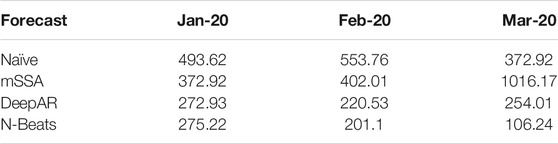
TABLE 2. Mean squared error.

3 Description of Gradual Increase

The main idea behind the method of Gradual Increase lies in the proper use of the warm start. When we have to handle a task a from Eq. 22, we can check whether it is possible to implement it with a smaller number of assets (or turbines within the assets). If it is possible, then the resulting solution can be used as a start in either a larger or the entire pool. We try to start with a minimum sub-pool capable of implementing the task and add assets to the pool with its consequent optimization, until the entire pool is achieved. When implementing this algorithm, it is important to ensure that the branch and bound trees will not be destroyed which is achieved by the parallel run of the problem containing all assets which is interrupted whenever a new feasible solution is found: the problem is fed with that new feasible solution and then, the optimization is resumed. This can be achieved by the usage of built-in callback functions within Gurobi. Some problems are so complex that even the best solver will not be able to find a feasible solution to it. However, Gradual Increase enables us to find a feasible solution for the entire pool from the solution of a subproblem. Formally, the method is as follows: let us assume that SubSet(0) ∈ 2^{1,…,#A}, where SubSet(0) is a first sub-pool of the whole pool. Then the first problem can be formulated as follows:

$\mathrm{m}\mathrm{a}\mathrm{x}\mathrm{i}\mathrm{m}\mathrm{i}\mathrm{z}\mathrm{e}\sum _{k\in \mathrm{S}\mathrm{u}\mathrm{b}\mathrm{S}\mathrm{e}\mathrm{t}\left(0\right)}{p}_k^{\top }\cdot x_k(25)$

$\mathrm{s}.\mathrm{t}.\sum _{k\in \mathrm{S}\mathrm{u}\mathrm{b}\mathrm{S}\mathrm{e}\mathrm{t}\left(0\right)}{A}_k\cdot x_k=a,(26)$

$B_k\cdot x_k\le b_k\forall k\in \mathrm{S}\mathrm{u}\mathrm{b}\mathrm{S}\mathrm{e}\mathrm{t}\left(0\right),(27)$

$x_k\left(I\right)\in \left\{\mathrm{0,1}\right\}\forall k\in \mathrm{S}\mathrm{u}\mathrm{b}\mathrm{S}\mathrm{e}\mathrm{t}\left(0\right).(28)$

As a warm start, for the first problem, the states of turbines (u) from the solution of the problems in the previous period can be chosen. Since #SubSet(0) < #A, the Problem Eqs 25–28 contains fewer variables and constraints than the initial problem and should be solved faster except for specific cases, e.g. when the pool is so small that it is overloaded. Having solved this problem we get a sequence of vectors ${\widehat{x}}_k^{(0)}$, k ∈ SubSet(0). Then, when we get a larger sub-pool SubSet(1) such that:

$\mathrm{S}\mathrm{u}\mathrm{b}\mathrm{S}\mathrm{e}\mathrm{t}\left(0\right)\subset \mathrm{S}\mathrm{u}\mathrm{b}\mathrm{S}\mathrm{e}\mathrm{t}\left(1\right)\text{\hspace{0.17em}and\hspace{0.17em}}\mathrm{S}\mathrm{u}\mathrm{b}\mathrm{S}\mathrm{e}\mathrm{t}\left(0\right)\ne \mathrm{S}\mathrm{u}\mathrm{b}\mathrm{S}\mathrm{e}\mathrm{t}\left(1\right).$

Hence, the following problem for j = 0 can be formulated:

$\mathrm{m}\mathrm{a}\mathrm{x}\mathrm{i}\mathrm{m}\mathrm{i}\mathrm{z}\mathrm{e}\sum _{k\in \mathrm{S}\mathrm{u}\mathrm{b}\mathrm{S}\mathrm{e}\mathrm{t}\left(j+1\right)}{p}_k^{\top }\cdot x_k(29)$

$\mathrm{s}.\mathrm{t}.\sum _{k\in \mathrm{S}\mathrm{u}\mathrm{b}\mathrm{S}\mathrm{e}\mathrm{t}\left(j+1\right)}{A}_k\cdot x_k=a,(30)$

$B_k\cdot x_k\le b_k\forall k\in \mathrm{S}\mathrm{u}\mathrm{b}\mathrm{S}\mathrm{e}\mathrm{t}\left(j+1\right),(31)$

$xk\left(I\right)\in \left\{\mathrm{0,1}\right\}\forall k\in \mathrm{S}\mathrm{u}\mathrm{b}\mathrm{S}\mathrm{e}\mathrm{t}\left(j+1\right),(32)$

$x_m.\mathrm{s}\mathrm{t}\mathrm{a}\mathrm{r}\mathrm{t}={\widehat{x}}_m^{\left(j\right)}\forall m\in \mathrm{S}\mathrm{u}\mathrm{b}\mathrm{S}\mathrm{e}\mathrm{t}\left(j\right).(33)$

Note that Eq. 33 is the warm start, i.e. we start with the feasible solution and if the pool SubSet(0) is not capable of performing the task a, then we start from scratch. Let us denote the optimal solution of Problem Eqs 29–33 as follows: ${\widehat{x}}_k^{(j+1)}$, k ∈ SubSet(j + 1). However, what about assets with k∉SubSet(j + 1)? For these cases, the following problems for k∉SubSet(j + 1) are solved:

$\mathrm{m}\mathrm{a}\mathrm{x}\mathrm{i}\mathrm{m}\mathrm{i}\mathrm{z}\mathrm{e}{p}_k^{\top }\cdot x_k(34)$

$\mathrm{s}.\mathrm{t}.A_k\cdot x_k=\mathbf{0},(35)$

$B_k\cdot x_k\le b_k,(36)$

$x_k\left(I\right)\in \left\{\mathrm{0,1}\right\},(37)$

and their solution is denoted as follows: ${\bar{x}}_k$, k∉SubSet(j + 1). Note that all Problems (34)–(37) can be solved in parallel and ${\sum }_{k=1}^{\#A}{p}_k^{\top }\cdot {\bar{x}}_k$ is an upper bound of Problem Eqs 21–24. And the solution:

${\widehat{z}}_k^{\left(j+1\right)}=\left\{\begin{array}{cc}{\widehat{x}}_k^{\left(j+1\right)},\hfill & k\in \mathrm{S}\mathrm{u}\mathrm{b}\mathrm{S}\mathrm{e}\mathrm{t}\left(j+1\right),\hfill \\ {\bar{x}}_k,\hfill & k\notin \mathrm{S}\mathrm{u}\mathrm{b}\mathrm{S}\mathrm{e}\mathrm{t}\left(j+1\right)\hfill \end{array}\right.$

is a feasible solution of Problem Eqs 21–24. So when we have sub-pools:

$\mathrm{S}\mathrm{u}\mathrm{b}\mathrm{S}\mathrm{e}\mathrm{t}\left(0\right)\subset \mathrm{S}\mathrm{u}\mathrm{b}\mathrm{S}\mathrm{e}\mathrm{t}\left(1\right)\subset \mathrm{S}\mathrm{u}\mathrm{b}\mathrm{S}\mathrm{e}\mathrm{t}\left(2\right)\subset \dots \subset \mathrm{S}\mathrm{u}\mathrm{b}\mathrm{S}\mathrm{e}\mathrm{t}\left(N\right)=\left\{\mathrm{1,2},\dots ,\#A\right\},$

then for j = 0, Problem Eqs 25–28 is solved and for j > 0, Problem Eqs 29–33 is solved. When a problem for some j has been solved and we find out that it is infeasible, then for j + 1 we will start from scratch; otherwise, we take the solution for j as a starting point for the problem for j + 1. These warm starts have enabled us to solve a large number of problems much faster than when we would just rely on the power of an open-source or commercial solver.

3.1 An Example

Figure 1 demonstrates the methodology of Gradual Increase with an example of a pool with seven assets. It is optimized in the following way: assuming that a sub-pool of the first three power plants is capable of performing the task, the optimization is started with solving Problem Eqs 25–28 for SubSet(0) = {1, 2, 3}, and Problems Eqs 34–37 are solved for k = 4, 5, 6, and 7, yielding ${\bar{x}}_4,{\bar{x}}_5,{\bar{x}}_6$, and ${\bar{x}}_7$. For SubSet(0), there is no warm start and Problem Eqs 25–28 is solved yielding ${\widehat{x}}_1^{(0)},{\widehat{x}}_2^{(0)}$, and ${\widehat{x}}_3^{(0)}$ (the blue color in the diagram). The vector $[{\widehat{x}}_1^{(0)},{\widehat{x}}_2^{(0)},{\widehat{x}}_3^{(0)},{\bar{x}}_4,{\bar{x}}_5,{\bar{x}}_6,{\bar{x}}_7]$ is a feasible solution of the system of the seven assets, and $[{\widehat{x}}_1^{(0)},{\widehat{x}}_2^{(0)},{\widehat{x}}_3^{(0)},{\bar{x}}_4,{\bar{x}}_5]$ is a warm start for the sub-pool with the five assets.

FIGURE 1

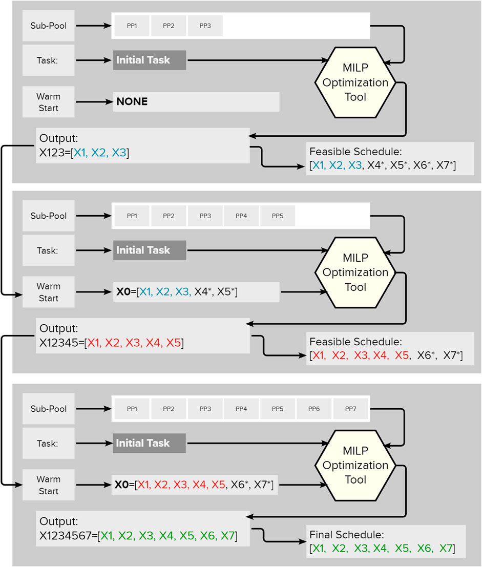
FIGURE 1. The visualization of the Gradual Increase methodology.

Then Problem Eqs 29–33 is solved for SubSet(1) = {1, 2, 3, 4, 5} yielding ${\widehat{x}}_1^{(1)},{\widehat{x}}_2^{(1)},{\widehat{x}}_3^{(1)},{\widehat{x}}_4^{(1)}$, and ${\widehat{x}}_5^{(1)}$ (the red color in the diagram). The vector $[{\widehat{x}}_1^{(1)},{\widehat{x}}_2^{(1)},{\widehat{x}}_3^{(1)},{\widehat{x}}_4^{(1)},{\widehat{x}}_5^{(1)},{\bar{x}}_6,{\bar{x}}_7]$ is both a feasible solution to the system with the seven assets, and a warm start for the sub-pool with the seven assets.

Then Problem Eqs 29–33 is solved for SubSet(2) = {1, 2, 3, 4, 5, 6, 7} yielding ${\widehat{x}}_1^{(2)},{\widehat{x}}_2^{(2)},{\widehat{x}}_3^{(2)}$, ${\widehat{x}}_4^{(2)}$, ${\widehat{x}}_5^{(2)}$, ${\widehat{x}}_6^{(2)}$, and ${\widehat{x}}_7^{(2)}$ (the green color in the diagram). The solution $[{\widehat{x}}_1^{(2)},{\widehat{x}}_2^{(2)},{\widehat{x}}_3^{(2)},{\widehat{x}}_4^{(2)},{\widehat{x}}_5^{(2)},{\widehat{x}}_6^{(2)},{\widehat{x}}_7^{(2)}]$ is the final output of Gradual Increase. Note that the task (Eq. 30) is the same for all sub-pools. In the first layer of the Gradual Increase methodology, there is no warm start. In the middle layer there is a warm start for the optimization and the output of this optimization is used as a warm start for a larger sub-pool. The last layer produces the final output. In the case of a time limit, it is possible to use one of the sub-optimal, but feasible solutions:

• $[{\widehat{x}}_1^{(0)},{\widehat{x}}_2^{(0)},{\widehat{x}}_3^{(0)},{\bar{x}}_4,{\bar{x}}_5,{\bar{x}}_6,{\bar{x}}_7]$,

• $[{\widehat{x}}_1^{(1)},{\widehat{x}}_2^{(1)},{\widehat{x}}_3^{(1)},{\widehat{x}}_4^{(1)},{\widehat{x}}_5^{(1)},{\bar{x}}_6,{\bar{x}}_7]$.

Figure 2 demonstrates an upgrade in the Gradual Increase methodology when there is a parallel run of the entire pool. This parallel run starts simultaneously with Gradual Increase and is interrupted when the latter finds a feasible solution. This feasible solution is fed to the parallel run without destroying branch and bound trees using callback functions, and after that, the optimization is resumed. This procedure repeats whenever Gradual Increase finds a new feasible solution as is shown in Figure 2. The number of such feasible solutions is equal to the number of the sub-pools.

FIGURE 2

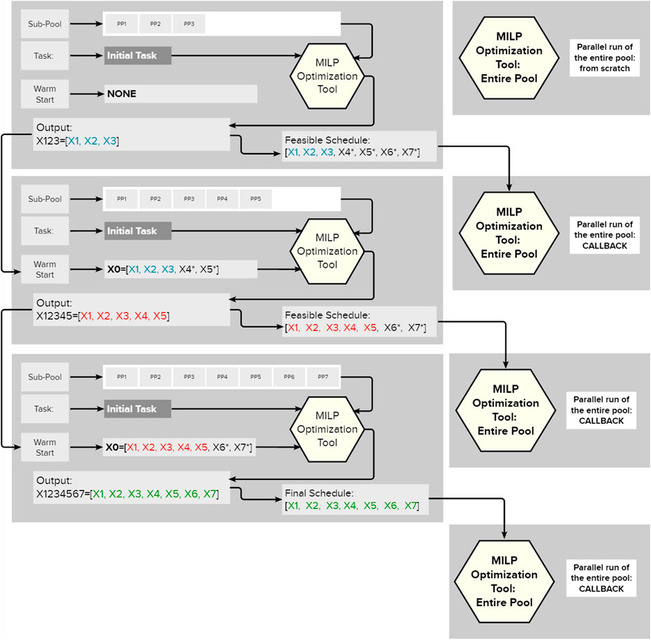
FIGURE 2. The visualization of the Gradual Increase methodology with a callback.

3.2 Further Improvements in Gradual Increase

When the same pool is optimized, then we can take the experience from previously solved problems in order to accelerate the solution of new problems as follows:

1. Exploration of which sub-pools would lead to a faster solution on previously solved problems and applying these sub-pools for new problems.

2. Exploration of the warm start: we can check if the binary variables from the previous problem can be used in the warm start: if it is possible then the first feasible solution will be obtained by means of LP otherwise the solver will start from scratch.

3. Exploration of what solver parameters from previously solved problems would lead to faster solutions of these problems and application of these parameters on the new problems. Results obtained by the Proximal Jacobian ADMM and Gradual Increase will be compared. We will also implement a hybrid of both methods.

4 Operation of the VPP Conducted on Historical Data

We consider systems with predefined assets as being part of the VPP, and historical prices and production together with their corresponding historical forecasts are applied. The wind production forecast is the task of the wind park: based on the prognosis the operators of the park inform the market operator that they are able to produce a specific schedule. The imbalance between the produced and predicted wind energy is the task of the flexible assets: the surplus of the wind production will be consumed by the batteries while the deficiency will be covered either by the biogas power plants or by discharging the batteries. This implementation will be conducted in the Model Predictive Control fashion where the problem is solved every 24 h when new information about prices and the weather arrives.

4.1 Model Predictive Control

Model Predictive Control (MPC) is a feedback control technique that naturally incorporates optimization (Moehle et al., 2019; Bemporad, 2006; Mattingley et al., 2011). In this study we consider certainty equivalent MPC and robust MPC proposed in Moehle et al. (2019). In certainty equivalent MPC, random quantities are replaced with predictions, and the associated optimization problem is solved to produce the schedule over the selected planning horizon. After optimization, the first power schedule is executed, i.e. the one associated with the time of optimization. For the next step, this process is repeated incorporating the updated information about price and imbalance forecasts. Following the notation from Table 1, our MPC algorithm is defined as follows:

Take the initial state State₀ of the system (storage levels and states of the turbines) as the first input.

for t = 1 to N do:

1. Forecast. Make price and imbalance forecasts that will be used as inputs in the optimization:

$\begin{array}{l}\hfill {\mathbf{F}\mathbf{r}\mathbf{c}}_t=\left[Fr{c}_t,Fr{c}_{t+1},\dots ,Fr{c}_{t+H-1}\right],\\ \hfill \mathrm{\Delta }{\mathbf{p}\mathbf{r}\mathbf{o}\mathbf{d}}_t^W=\left[\mathrm{\Delta }pro{d}_t^W,\mathrm{\Delta }pro{d}_{t+1}^W,\dots ,\mathrm{\Delta }pro{d}_{t+H-1}^W\right].\end{array}$

2. Optimize. Solve the dynamic optimization problem:

$\mathrm{V}\mathrm{P}\mathrm{P}\left({\mathbf{F}\mathbf{r}\mathbf{c}}_t^{\left(\mathrm{D}\mathrm{A}\right)},{\mathbf{F}\mathbf{r}\mathbf{c}}_t^{\left(\mathrm{I}\mathrm{D}\right)},\mathrm{\Delta }{\mathbf{p}\mathbf{r}\mathbf{o}\mathbf{d}}_t^W,{\mathbf{S}\mathbf{t}\mathbf{a}\mathbf{t}\mathbf{e}}_{t-1}\right),(38)$

where price_t determines the objective value and ${\mathbf{p}\mathbf{r}\mathbf{o}\mathbf{d}}_t^W$ determines the right-hand side of the power production constraints. Solving this optimization problem yields the decision vector.

y_t = [y_t, y_t+1, … , y_t+H−1].

3. Execute only y_t from the whole vector y_t because this decision relates to the most up-to-date time step. The rest of the ys in the y is discarded.

4. Determine the value Revenue_t which is the revenue associated with the execution of y_t which equals

$Revenu{e}_t={\mathrm{V}\mathrm{P}\mathrm{P}}_{rv}^{\left(h\right)}\left({\mathbf{S}\mathbf{p}\mathbf{t}}_t^{\left(\mathrm{D}\mathrm{A}\right)},{\mathbf{S}\mathbf{p}\mathbf{t}}_t^{\left(\mathrm{I}\mathrm{D}\right)},\nabla pro{d}_t^W\right)(39)$

and the next state is:

${\mathbf{S}\mathbf{t}\mathbf{a}\mathbf{t}\mathbf{e}}_t=f\left({\mathbf{S}\mathbf{t}\mathbf{a}\mathbf{t}\mathbf{e}}_{t-1},y_t,\nabla pro{d}_t^W\right),(40)$

where f is a linear function which determines the updates of the storage levels and states of the turbines according to Eqs, 6, 14, 8, 9.

end for.

Thus, our ultimate goal is the maximization of the sum:

$\mathrm{T}\mathrm{o}\mathrm{t}\mathrm{R}\mathrm{e}\mathrm{v}=\sum _{t=1}^{N}Revenu{e}_t\to \max ,(41)$

i.e. the solution of the problems VPP(⋅, ⋅, ⋅) is an intermediate goal aimed at maximizing the value TotRev. And in this study the model is assessed in terms of the value of TotRev and the total speed-up. All the methods only differ by the approach to problems VPP(⋅, ⋅, ⋅) and the following will be applied:

1. Generic Approach: we rely on the power of the solver without any decomposition or splitting.

2. Gradual Increase: asset-wise decomposition is performed as it is shown in the description of the method and in a similar way this approach is applied on the turbines within each biogas power plant.

3. Proximal Jacobian ADMM: we start with LP relaxation in order to ensure that the coupling constraint is satisfied and then apply MILP methods to sub-pools (most on single power plants) in order to extract an integral solution.

4. Partial Integrality: at time t, we relax all integral constraints of all variables y_t+1, y_t+2, … , y_t+H−1. This leads to a significant reduction of binary variables while providing a feasible action y_t. (Variable y_t is defined in Table 1.).

5. Management of Timing Constraints by Penalization: in many situations, timing constraints can be enforced by imposing high penalties on switch-ons and switch-offs. This enables us to get rid of most of our inequality constraints and thereby to significantly accelerate the calculations.

6. Parameter tuning with MPC: within MPC, we can run parameter tuning of the solver after we have solved a problem. It can be conducted parallel to the solution of the new problems. After solving 20 problems, the tuning parameters of the solver are adjusted which provides further speed-up. In Python’s Gurobi environment, this can be conducted by means of the operation Model.tune().

7. Hybrid of GI and Proximal Jacobian ADMM: instead of adding single power plants in the pool they are added by blocks and in order to solve block subproblems faster, we apply Gradual Increase.

4.2 Robust Model Predictive Control

The difference between MPC and RMPC lies in a different approach to the second step of the algorithm (Optimize). In Eq. 38, there is a single forecast of prices and imbalances. In RMPC however (Moehle et al., 2019), we use a predefined number of scenarios M, i.e.

${\mathrm{S}\mathrm{c}\mathrm{e}\mathrm{n}\mathrm{a}\mathrm{r}\mathrm{i}\mathrm{o}}_m=\left({\mathbf{F}\mathbf{r}\mathbf{c}}_t^{\left(\mathrm{D}\mathrm{A},m\right)},{\mathbf{F}\mathbf{r}\mathbf{c}}_t^{\left(\mathrm{I}\mathrm{D},m\right)},\mathrm{\Delta }{\mathbf{p}\mathbf{r}\mathbf{o}\mathbf{d}}_t^{\left(W,m\right)}\right)\text{\hspace{0.17em}for\hspace{0.17em}}m=\mathrm{1,2},\dots ,M,$

and use each scenario m in order to solve the maximization problem:

$\begin{array}{ccc}\hfill \sum _{m=1}^M\mathrm{V}\mathrm{P}\mathrm{P}\left({\mathbf{F}\mathbf{r}\mathbf{c}}_t^{\left(\mathrm{D}\mathrm{A},m\right)},{\mathbf{F}\mathbf{r}\mathbf{c}}_t^{\left(\mathrm{I}\mathrm{D},m\right)},\mathrm{\Delta }{\mathbf{p}\mathbf{r}\mathbf{o}\mathbf{d}}_t^{\left(W,m\right)},{\mathbf{S}\mathbf{t}\mathbf{a}\mathbf{t}\mathbf{e}}_{t-1}\right)& \hfill & \hfill \end{array}(42)$

$\begin{array}{ccc}\hfill p_{\tau ,k,i}^{\left(\mathrm{I}\mathrm{D},\widehat{m}\right)}-p_{\tau ,k,i}^{\left(\mathrm{I}\mathrm{D},\bar{m}\right)}=0\forall k,i\text{\hspace{0.17em}and\hspace{0.17em}}\forall \widehat{m},\bar{m}\le M\text{\hspace{0.17em}and\hspace{0.17em}}\forall \tau \le h,& \hfill & \hfill \end{array}(43)$

$\begin{array}{ccc}\hfill p_{\tau ,k,i}^{\left(\mathrm{D}\mathrm{A},\widehat{m}\right)}-p_{\tau ,k,i}^{\left(\mathrm{D}\mathrm{A},\bar{m}\right)}=0\forall k,i\text{\hspace{0.17em}and\hspace{0.17em}}\forall \widehat{m},\bar{m}\le M\text{\hspace{0.17em}and\hspace{0.17em}}\forall \tau \le h,& \hfill & \hfill \end{array}(44)$

where the sum in Eq. 42 means that we add up all the objectives from the problems $\mathrm{V}\mathrm{P}\mathrm{P}\left({\mathbf{F}\mathbf{r}\mathbf{c}}_t^{(\mathrm{D}\mathrm{A},m)},{\mathbf{F}\mathbf{r}\mathbf{c}}_t^{(\mathrm{I}\mathrm{D},m)},\mathrm{\Delta }{\mathbf{p}\mathbf{r}\mathbf{o}\mathbf{d}}_t^{(W,m)},{\mathbf{S}\mathbf{t}\mathbf{a}\mathbf{t}\mathbf{e}}_{t-1}\right)$ for each m and maximize their sum; as for the constraints, they all are added into the set of the constraints of the resulting problem. The constraints Eqs 43, 44 ensure that the power produced within each scenario Scenario_m will be the same up to time h. This also ensures that the execution in Eq. 39 will be the same for all the scenarios. The rest of the steps of the MPC algorithm remain unchanged. It can easily be shown that the same power values for all scenarios also imply the same states of the turbines and the same storage levels for all the scenarios when t < h.

5 Data Inputs Into Optimization

As the objective function Eq. 1 and coupling constraints Eq. 19 suggest, the optimization requires data inputs, i.e. forecasts, and is conducted sequentially: at the start of the new period, Problem Eq. 38 is solved taking into account the state of the system. Then the real prices and imbalances become known and the solution of Eq. 39 enables us to calculate the real revenue yielded by solving Eq. 38. Then the state of the system is updated by (40), and the process resumes. Hence, the following data inputs are required:

• Historical prices on the EEX market and associated historical forecasts

• Historical wind production from the considered wind parks and associated historical forecasts

As for price inputs, we apply commercial forecasts. Since these forecasts are not available for a large audience, we propose three forecasting methods based on Deep Learning whose implementation is possible using open-source software. The following subsection specifies what price forecasts are employed apart from the commercial ones.

5.1 Price Inputs

Following developments in machine learning research for time series forecasting, we consider several state-of-the-art machine and Deep Learning approaches for the modeling of electricity prices:

• Multivariate Singular Spectrum Analysis (mSSA)—a popular and widely used time series forecasting method. As demonstrated in Agarwal et al. (2020), mSSA was found to outperform deep neural network architectures such as LSTM and DeepAR in the presence of missing data and noise level.

• DeepAR—a methodology (developed by Amazon Research) for producing accurate probabilistic forecasts, based on training an auto-regressive recurrent network model (Salinas et al., 2019). We use GluonTS Alexandrov et al. (2020) implementation of DeepAR for our experiments.

• N − BEATS—a deep neural architecture based on backward and forward residual links and a very deep stack of fully-connected layers (Oreshkin et al., 2020). The architecture demonstrated good performance in M4 forecasting competitions and more recently (Oreshkin et al., 2020) has been used for electricity load forecasting.

5.2 Production Inputs

Historical imbalances are obtained as the difference between the real aggregate production and the forecasted aggregate production. The aggregate production for both cases is obtained by adding up the productions from each wind turbine. For the aggregate production of wind, commercial forecasts are used. The prediction of imbalances would exceed the scope of this paper and in this study, the imbalances are treated as follows:

• Usage of historical imbalances as inputs—an assumption of a perfect foresight.

• Fitting imbalances with an ARMA process and the simulation of them within an RMPC scheme.

In the exploration of the speed of the optimization algorithms (Subsection 7.4), the commercial price forecasts are employed and the imbalances are assumed to be known in advance. In the exploration of the precision (Subsection 7.3), all proposed price forecasts are employed and where imbalances are assumed to be uncertain, the optimization is conducted within RMPC.

6 Nuances of the Optimization

We optimize against prices which implies that turbines should produce when the price is high, and be off when it is low. As for the battery, it should discharge when the price is high, and it should charge the battery when it is either low or negative.

Note that at the moment of optimization, the spot prices are not known and thus the decision-making relies on forecasts.

6.1 The Choice of Sub-Pools

At time t, the optimal solution from time t − 1 is taken and the following arrays are calculated:

$P_k=\sum _{i=1}^{\mathrm{\#}\mathrm{U}\left(k\right)}\sum _{\tau =1}^T{p}_{\tau ,k,i}^{\text{ID}},k\in \left\{\mathrm{1,2},\dots ,\#A\right\},(45)$

$P_{k,i}=\sum _{\tau =1}^T{p}_{\tau ,k,i}^{\text{ID}},k\in \left\{\mathrm{1,2},\dots ,\#A\right\},i\in \left\{\mathrm{1,2},\dots ,\#U\left(k\right)\right\}.(46)$

So when choosing which power plant to add to the sub-pool, we prefer such power plants k for which P_k is larger. When choosing a power plant k as part of the pool, we decide which turbines to add first according to the values P_k,i, i.e. the higher values of P_k,i are preferred. Since the optimization is run every 15 min, in many cases there is not a very significant difference between the problems at time t and t − 1 and this is one of the ways to exploit it.

6.2 Hardware and Solvers

We use m5d.4xlarge EC2 instance within Amazon Web Services i.e. 16 vCPUs and 64 GiB RAM. In optimization, two solvers are employed: CBC and Gurobi. In order to optimize our set of assets, we can get by with CBC, but in order to deal with portfolios of replicated biogas power plants, it is necessary to resort to the commercial solver Gurobi.

6.3 Implementation of Proximal Jacobian ADMM

The proximal Jacobian ADMM (Alternating Direction Method of Multipliers) was developed in Deng et al. (2017) and Wei and Ozdaglar (2013) and its convergence for linear programming problems was proven in the same literature. In this study apart from Gradual Increase, Proximal Jacobian ADMM is used, where first all integrality constraints are relaxed, and the algorithm iterates until the acceptable violation of coupling constraints is achieved: the preservation of the rest of the constraints is provided by the subproblems. After finishing the linear programming part we get the action vectors ${\widehat{x}}_k$, for each k ∈ {1, 2, … , #A}. Let ${\widehat{a}}_k$ denote $A_x\cdot {\widehat{x}}_k$, i.e. ${\widehat{a}}_k=A_x\cdot {\widehat{x}}_k$. Then for each asset k, the mixed-integer action vector is recovered by solving the following subproblems.

$\mathrm{m}\mathrm{a}\mathrm{x}\mathrm{i}\mathrm{m}\mathrm{i}\mathrm{z}\mathrm{e}{p}_k^{\top }\cdot x_k(47)$

$\mathrm{s}.\mathrm{t}.A_k\cdot x_k={\widehat{a}}_k,(48)$

$B_k\cdot x_k\le b_k,(49)$

$x_k\left(I\right)\in \left\{\mathrm{0,1}\right\}.(50)$

Sometimes these problems are infeasible, but this can be handled as follows: if $\mathcal{K}$ is a subset of {1, 2, … , #A} such that for each $k\in \mathcal{K}$ the problem Eqs 47–50 is infeasible, then we can solve

$\mathrm{m}\mathrm{a}\mathrm{x}\mathrm{i}\mathrm{m}\mathrm{i}\mathrm{z}\mathrm{e}\sum _{k\in \mathcal{K}}{p}_k^{\top }\cdot x_k(51)$

$\mathrm{s}.\mathrm{t}.\sum _{k\in \mathcal{K}}{A}_k\cdot x_k=\sum _{k\in \mathcal{K}}{\widehat{a}}_k,(52)$

$B_k\cdot x_k\le b_k,x_k\left(I\right)\in \left\{\mathrm{0,1}\right\}\forall k\in \mathcal{K}.(53)$

In all our problems $\#\mathcal{K}\le 4$ and such pools are solved in a matter of seconds. However this procedure provides sub-optimal solutions, but this technique is amenable to parallelization (Wei and Ozdaglar, 2013) and can handle extra-large pools of assets. It can also be easily shown that this algorithm can be combined with Gradual Increase.

6.4 Parallelization

Parallelization is crucial in optimizing these kinds of virtual power plants. And when applying any aforementioned methods, we propose using two independent machines where the first machine runs the problem from scratch uninterrupted and the second machine starts from scratch but gets interrupted when decomposition, splitting, or pruning methods find a new feasible solution and then, with a new start, they resume the calculations, having preserved all the branch and bound trees. When any method gets the confirmation that there is the optimal solution, then all other cores terminate. The same happens when the time limit is expired. In this case of all feasible solutions found by all methods, we choose the one which yields the largest value of the objective function. The usage of an independent and uninterrupted core is proposed in order to make sure that decomposition methods will not lead to longer computation times. This can happen in situations when a solver was capable of finding the optimal solution almost immediately and most of the time was spent on the confirmation that the solution is optimal. In such special cases, GI would only decelerate the total computation time but it will not happen if it is coupled with such a core. The utilization of an interrupted machine is proposed in order to preserve branch & bound trees: each feasible solution can enrich the search space.

7 Results

This section presents the results of the calculations related to the speed (Subsection 7.4), forecast precision in terms of MSE (Subsection 7.1), and the optimality in a stochastic environment (Subsection 7.3). In both cases, we consider the following period: 2020/1/1–2020/9/26. In the case of the speed, the prediction horizon (H) is 2 days ahead. In the case of optimality, our prediction horizon (H) is 3 days ahead. In both cases, the execution horizon (h) is 24 h. Price forecasts are updated once or two times per day, but production forecasts are updated every 15 min. Therefore, it is crucial to be able to solve every optimization problem in maximum 15 min, otherwise it will not be possible to deploy these algorithms for real-time applications.

In the case of the speed, only state-of-the-art commercial price forecasts are used and perfect knowledge of the imbalance is assumed. We emphasize that the size of imbalance increases proportionally to the number of assets; otherwise, the optimization problem would be trivial. In addition, in the case of the speed, timing constraints are introduced and for each turbine, UT and DT are generated by means of a uniformly distributed random variable taking values: 0, 1, 2, 3, 4. In the case of optimality, we consider different forecast methods described in Section 5 affect the cumulative revenue over the aforementioned period.

7.1 Analysis of Price Forecasts

We apply the above models to generate and benchmark forecasts 168-h ahead at three time points: 1) 31-Dec-2020 2) 31-Jan-2021 3) 29-Feb-2021. Our approach is to demonstrate benefits from using machine and Deep Learning forecasting technologies, rather than a comprehensive evaluation of different classes of methods or to add to the debate on the benefits of machine learning vs. statistical algorithms. We generate forecasts for 168 h (7 days) ahead and benchmark forecasts against 168 h lagged naive forecasts that is able to capture daily and hourly dynamics of electricity prices (thus is a competitive benchmark in the short-term, especially as our forecasts are of parsimonious nature and only use historic price information).

We have utilized mean squared error (MSE) to measure the performance of considered forecasting frameworks to obtain the following results in Table 2. Our results demonstrate significant benefits (as measured by forecasting value added—FVA) from applying powerful Deep Learning frameworks such as DeepAR and N-Beats, as well as data-driven models such as mSSA that are able to capture dynamic and feature-rich behavior of electricity prices. The applied frameworks are able to demonstrate, even without any hyper-parameter optimization, that powerful open-source frameworks such as mSSA, DeepAR and N-Beats are able to generate (see Table 4) very competitive forecasting inputs in comparison with expensive commercial forecast feeds.

7.2 Analysis of Results in Terms of Decision Variables

This subsection demonstrates results in terms of decision variables and input parameters. In the optimization models presented in this paper, there are the following variables: p, u, v, w, soc (See Table 1). Instead of visualizing all the variables, we concentrate on the most important ones. Let us note first, that the variables p and u (i.e. p_t,k,i and u_t,k,i, ∀t, k, i) are interrelated: for turbines, Eq. 4 implies that if p_t,k,i > 0 then u_t,k,i = 1, and if p_t,k,i = 0, then u_t,k,i = 0; for batteries, Eq. 10 implies that if $p_{t,k,1}^d>0$, then u_t,k,1 = 1, and if $p_{t,k,1}^d=0$, then u_t,k,i = 0. Since u is derived from p, it will not be visualized, because all the information about it is contained in p. The variables $p_{t,k,1}^d$ and $p_{t,k,1}^c$ are interrelated because only one of them can be positive, i.e. if one of them is positive, then the other is zero which is entailed by Eqs 10, 11. This is because the considered batteries cannot charge and discharge at the same time (Alqunun et al., 2020). Therefore in a battery according to Eq. 18, if p_t,k,1 = 0, then both $p_{t,k,1}^d$ and $p_{t,k,1}^c$ are zero; if p_t,k,1 > 0, then $p_{t,k,1}^d>0$ and $p_{t,k,1}=p_{t,k,1}^d$; if p_t,k,1 < 0, then $p_{t,k,1}^c>0$ and $p_{t,k,1}=-p_{t,k,1}^c$. Thus, all the information about u_t,k,i, $p_{t,k,1}^d$, and $p_{t,k,1}^c$ is contained in p_t,k,i ∀t, k, i. According to Eq. 6 and Eq. 14, the storage levels are uniquely determined by the power output and the initial storage level, however they are visualized in Figure 3, in order to show how they can restrict the power output. Based on the aforementioned considerations, the following variables will be visualized:

• The aggregate power output: i.e the left-hand side the coupling constraints, i.e. Eq. 19.

• The aggregate storage level in both biogas power plants and batteries.

• The power output for a single power plant in order to demonstrate the effect of timing constraints.

FIGURE 3

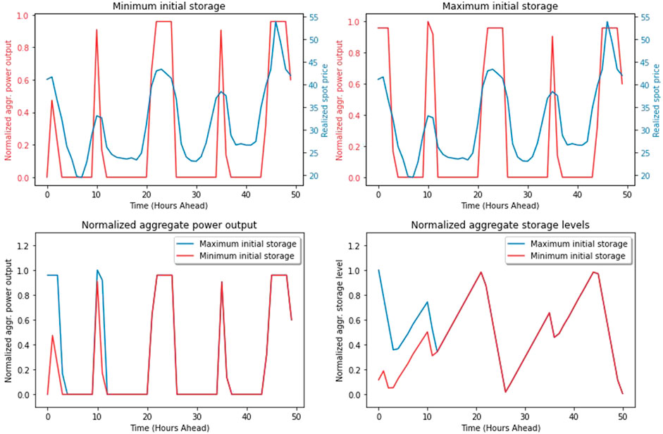
FIGURE 3. The dependence of the total power output on forecasted prices and initial storage levels.

Due to confidentiality issues, the schedules and storage levels are normalized. Figures 3, 4 are obtained from the optimization of a system that consists of three real assets mentioned in Subsection 2.1 and one asset with randomly generated parameters. For the sake of clarity of the figures, only day-ahead schedules and day-ahead prices are considered in Subsection 7.2.1 and Subsection 7.2.2.

FIGURE 4

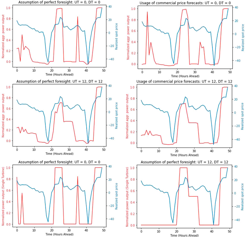
FIGURE 4. The dependence of the revenue on the quality of the forecasts and timing constraints.

7.2.1 The Dependence of the Total Power Output on Forecasted Prices

Figure 3 visualizes the schedules for the maximum and minimum initial storage levels and all of them are normalized. These are aggregate power and storage level schedules. The former is visualized against spot prices. In the corresponding optimization problem, the price input is historical spot prices, i.e. the optimization is implemented under perfect foresight. In this example for the price input, we apply 50 consecutive day-ahead spot prices from the EEX market starting on 08. 04. 2020 at 9:00 PM, and the analogous inputs are used for the imbalances. In the top part of Figure 3, there are two scales: the scale associated with the aggregate schedule (red) and the scale associated with the spot prices (blue). Note that in both top left and top right parts of Figure 3, when the price is high, the aggregate power output tends to be high, which is natural because the scalar product of the red (non-normalized) line and the blue lines is part of the objective which is maximized. In other words, the role of the optimization is to cherry-pick high prices, but it can be disabled by the constraints and the state of the system. For example, in the top left part of Figure 3, the first price is relatively high, but no power is produced because there is not enough fuel for it (minimum initial storage), while in the top right part of this figure there is the maximum initial storage, therefore the power is produced. The bottom-left and bottom-right parts of Figure 3 visualize schedules and storage levels for the maximum and minimum initial storage levels, respectively. Let us note that at hour 10, there is a local maximum in the spot price. In the case of the maximum initial storage, there is more power generated at hours 10 and 11, than in the case of the minimum initial storage because the fuel was stored in order to be used later when the prices are higher. In the bottom right part of Figure 3, the storage starts at a non-zero level. This is because there is a minimum initial storage level for which it is possible to satisfy the coupling constraint.

7.2.2 The Dependence of the Revenue on the Quality of the Forecasts

The top left part of Figure 4 visualizes a power schedule against corresponding spot prices under perfect foresight. The top right part of Figure 4 visualizes a schedule against corresponding spot prices under the usage of commercial price forecasts. The forecasts of the spot prices were generated on 05. 30. 2020 at 12:00 AM and the price vector is 50 consecutive hourly price forecasts starting at 9:00 PM on 05. 30. 2020. Let us note that between hours 30 and 40 where there is a local maximum spot price, the schedule was adjusted to this maximum, i.e. there is a spike in the aggregate power production. However the commercial price forecasts have not predicted the local maximum price at that point, therefore there is no spike in the power production in the left part of the picture. Let us also note that the spot price is negative in the following chunks:

• During hours 17–21,

• During hours 41–43.

In the top left and middle parts of Figure 4, the aggregate power output is negative at the chunks where the price is negative. This is enabled by Eq. 18, and when the price is negative then the battery is charged. The commercial forecasts have not predicted these negative prices. Instead, these forecasts values are close to zero which results in “doing nothing” at these chunks. This emphasizes the importance of the quality of the forecasts.

The middle part of Figure 4 visualizes the normalized aggregate schedules for the system where all the turbines have the following parameters of the timing constraints: UT = DT = 12.

The bottom part of Figure 4 visualizes the normalized schedule of the first turbine of the fourth asset in the pool for perfect foresight. In the bottom-left part of Figure 4, there are no timing constraints. In the bottom right part of Figure 4, there is UT = DT = 12.

Let us note that any switch-on of a turbine is associated with a guaranteed loss of fuel. For example, let $\mathcal{I}$ denote a subset of all turbines of Asset k. Then the switch-on of all the turbines within $\mathcal{I}$, yields the following guaranteed minimum usage of the fuel within the storage of Asset k:

$\sum _{i\in \mathcal{I}}{\mathrm{P}\mathrm{m}\mathrm{i}\mathrm{n}}_{k,i}\ast {\mathrm{U}\mathrm{T}}^{\left(k,i\right)},$

which implies that the loss of fuel is proportional to UT. This is the reason why in the bottom right part of Figure 3, it was impossible to cherry-pick the local maximum spot price at time 36: the turbine was switched on at hour 21 and was on until hour 32. At hour 32, the storage was almost empty, therefore the turbine had to be switched off. In 3 hours there was that local maximum price, but there was not enough fuel in the storage. In addition to this, DT = 12 which makes it impossible to switch on that turbine. We have also calculated the schedule for UT = 12 and DT = 0. In this case, it is possible to switch on the turbine after hour 32, but it was not implemented, because this switch-on would enable us to cherry-pick the local maximum at time 36, which is 10.96 euros, but at hour 42, the price is −48.17 euros, and this “bonus” is inevitable, if the turbine is switched on after hour 32.

In the top left part of Figure 4, there are no timing constraints and there is perfect foresight, therefore there is the largest revenue. In the top right part of this figure, there are no timing constraints, but the prices are not known. Hence the revenue there is 91.73% of the maximum. In the middle left part of this picture, there is perfect foresight, but there are timing constraints, i.e. UT = DT = 12. And the revenue for this case is 91.19% of the maximum. In the middle right part of Figure 4, there are timing constraints and the prices are forecasted. The revenue for this case is 85.22% of the maximum.

Hence, in order to increase the revenues, apart from optimization methods, it is important to:

1. Improve price forecasts.

2. Perform technological advances on turbines in order to reduce UT and DT, if it is possible.

7.3 Optimality

When we explore the optimality, we attempt to get as close as possible to the total revenue that we would achieve in the case of perfect foresight, when both prices and imbalances are known in advance. So, the cumulative revenues under perfect foresight is our benchmark and we explore the percentage of it provided by different methods. We explore this by means of variable σ from Eq. 20, which is apparently the unit in the case of perfect foresight. Table 4 summarizes the σ-values. We can observe that when we use commercial state-of-the-art forecasts and assume perfect foresight of productions, then RMPC yields slightly higher revenues. In the case of uncertain productions, we utilize only RMPC because we prefer simulations of the realizations of productions rather than trying to find a point forecast: the forecast of the imbalance is a challenging task and the exploration of it exceeds the scope of this paper. But mimicking this imbalance by ARMA processes yields σ equal to 84.19% if we use commercial forecasts and σ equal to 81.29% if we use mSSA, which can be achieved by utilizing open-source software.

7.4 Speed

When we explore the speed, our benchmark is the time needed to solve the MILP problem by the Gurobi solver. We call this approach the Brute Force and the proposed decomposition and splitting algorithms must enable us to find the solution faster. In real-time applications, an optimization problem is solved every 15 min. Some of these problems require so much time to be solved that we either do not get any feasible solution or get a solution that is highly sub-optimal. In Subsection 7.4.1 only such cases are explored. We are interested in maximum improvement provided by Gradual Increase compared to the situation when we rely only on the speed of the solver. Subsection 7.4.2, considers all problems and judges the improvements in terms of average calculation time. Apart from Gradual Increase, Subsection 7.4.2 considers other methods and their hybrids with Gradual Increase.

7.4.1 Maximum Improvements in Calculation Times

The period 2020/1/1–2020/9/26 contains 269 days. Thus, for each considered pool, 269 problems are solved. Table 3 summarizes average calculation times and Column #Assets indicates how many assets were involved in optimization. For the pool with 200 assets, out of 269 problems, 7 were not solved in 15 min, i.e. no feasible solution was found within this period, however Gradual Increase enabled us to get a feasible solution with the relative error (MIPgap) bounded by 1% and in one case optimality message was obtained (MIPgap ≤0.01%). In that case, the time limit is removed and the problems were solved by Brute Force and Gradual Increase. The former required 24,789 s and the latter took only 128.4 s, i.e. the Gradual Increase solved the problem approximately 193 times faster. We also explored how the objective is improved by the utilization of Gradual Increase in these cases for 15 and 5 min: it is desirable to run optimization faster than in 15 min in order to enable traders to make judgments. The best improvement in the objective value under the time limit of 15 min provided by Gradual Increase is 36 times, i.e. the objective value by Gradual Increase is 36 times larger than that of Brute Force. Under the time limit of 5 min, this improvement is 78 times.

TABLE 3

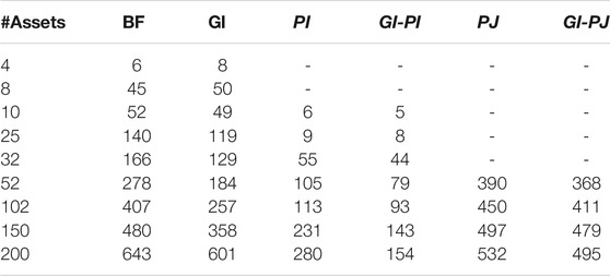
TABLE 3. Average speed of calculations (in seconds) for methods: BF, Brute Force; GI, Gradual Increase ; PI, Partial Integrality; GI-PI, Combination of Gradual Increase and Partial Integrality; PJ, Proximal Jacobian ADMM; GI-PJ, Combination of Gradual Increase and Proximal Jacobiand ADMM.

7.4.2 Improvements in Average Time

Table 3 summarizes the average calculation times provided by different methods. The headers of each column refer to the method applied and the caption of the table explains the abbreviations in the headers. The methods in the headers with italic font are the techniques which yield sub-optimal solutions but the resulting value of TotRev yielded around 99.96% of the maximum. Such methods are: partial integrality, partial integrality coupled with Gradual increase, proximal Jacobian ADMM, and proximal Jacobian ADMM coupled with Gradual increase. The methods such as Brute Force and Gradual increase lead to the optimal solution provided the solver has enough time. In Table 3, it can be observed how Gradual increase (GI) outperforms Brute Force (BF) in terms of time. When we solve problems by Brute Force, we only have the time limit of 15 min, i.e. the computations finish if either the optimal solution is found (the relative difference between the upper and the lower bound is below 0.01%) or the time limit has expired. In columns BF, GI, PI, and GI-PI we try to get the optimality message within 15 min. As for methods based on ADMM, this approach is irrelevant and the stopping criteria for these algorithms are described in Subsection 6.3. So in Table 3, it can be observed that GI improves over BF when the number of assets is increased, but when it gets closer to 200 then the difference is smaller. This is because the process finishes either when the optimal solution is found or when the time limit is exceeded. Thus the more assets we have in the portfolio, the more cases we face when the computation time expires. As stated above, GI helps us find the optimal solution, but it has nothing to do with the confirmation of the optimal solution (calculation of upper bounds). In order to accelerate this confirmation, we can resort to Partial Integrality. In this case, we do not get to the expiration of the time limit and the fastest method turned out to be the combination of Gradual Increase and Partial Integrality which yields average calculation time 4.17 times smaller than that of Brute Force. The method Proximal Jacobian ADMM is relevant only for large pools of assets, therefore we started calculations from 52 assets in the pool. And we can see that Brute Force outperforms this method in terms of speed for 52, 102, and 150. But when we have 200 assets, then Proximal Jacobian ADMM outperforms Brute Force. When Proximal Jacobian ADMM and Gradual Increase are combined, then we get further acceleration (column GI-PJ) for 200 assets—approximately 1.3 times faster than Brute Force. Another positive side of Proximal Jacobian ADMM is that it imposes lighter memory requirements on the machine than other proposed methods (Boyd et al., 2011).

Conclusion

In this paper we have presented optimization and forecast algorithms with the goal of more efficient management of the virtual power plants and the by-product of such algorithms is the facilitation of the integration of Distributed Energy Resources into the grid. In other words, one of the ways to profit from owning a DER resource is connecting it to an efficiently optimized virtual power plant. The analysis in terms of decision variables revealed how timing constraints and the precision of price forecasts affect the revenue. We have explored the computation times of GI and Proximal Jacobian ADMM dependent on the number of biogas power plants. The main point of these calculations is that the presented algorithms are able to handle up to hundreds of power plants within a pool if we properly use decomposition and splitting methods (or their combination). We also learned that the combination of Gradual Increase with Partial Integrality yields further improvements in computation time. Similar results are achieved when we combine Gradual Increase with Proximal Jacobian ADMM. We have also conducted experiments with a pool of two biogas power plants and a single battery in order to compare different forecasts (Commercial state-of-the-art, mSSA, DeepAR, N-BEATS) and optimization methods (MPC and Robust MPC). The usage of Robust MPC yielded the revenue 0.447% higher than that of MPC, therefore in our future research, we will consider combining Robust MPC with decomposition methods in order to achieve analogous results for larger pools. When the VPP is optimized by means of RMPC under price and imbalance uncertainty, then the utilization of commercial price forecasts yields 84.19% of the maximum possible revenue whilst the usage of our mSSA forecasts yields 81.29% of it. However, this forecast can be achieved by using of open-source software. All the optimization calculations related to Table 4 were conducted with CBC solver. The ability to run virtual power plants by means of open-source software also facilitates balancing and the incorporation of newly distributed energy resources into the grid. However, there is still the need for commercial solvers when we deal with large systems consisting of hundreds of assets.

TABLE 4

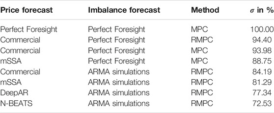
TABLE 4. The σ-value for MPC/RMPC and different forecast methods.

Data Availability Statement

The data analyzed in this study is subject to the following licenses/restrictions: We have the data for two biogas power plants and a battery. We also have data for wind parks. We disclose neither of these assets due to confidentiality issues. We also use commercial forecasts of prices and weather and this information is also confidential. Requests to access these datasets should be directed to vadim.omelcenko@alpiq.com.

Author Contributions

All authors listed have made a substantial, direct, and intellectual contribution to the work and approved it for publication. The contribution of the first author is optimization methods and the modeling of the VPP. The contribution of the second author is price forecasting models.

Funding

This project has received funding from the European Union’s Horizon 2020 research and innovation program under grant agreement No 883710.

Conflict of Interest

Author VO was employed by the company Alpiq Services CZ s.r.o.

The remaining author declare that the research was conducted in the absence of any commercial or financial relationships that could be construed as a potential conflict of interest.

Publisher’s Note

All claims expressed in this article are solely those of the authors and do not necessarily represent those of their affiliated organizations, or those of the publisher, the editors and the reviewers. Any product that may be evaluated in this article, or claim that may be made by its manufacturer, is not guaranteed or endorsed by the publisher.

Acknowledgments

The authors want to thank Alexandre Juncker, Frederik Grüll, Mohammadreza Saeedmanesh, Olle Sundström, Kévin Férin, Ronan Kavanagh, Christopher Hogendijk, Lemonia Skouta, Dimitri Nüscheler, Stefan Richter, Aleksejs Lozkins, Giovanni F. Campuzano Arroyo (UT), Sergey Ivanov (MAI), Gianluca Lipari (RWTH), Anish Agarwal (MIT), and Abdullah AlOmar (MIT) for inspiring discussions and technical support.

Appendix

Biogas plants are running on gas made from natural waste. Traditionally, they were built to run baseload, but the German government has now introduced some incentives so that they can run during peak hours. For that, they increase the installed capacity of the turbines and build a gas storage on-site. With the same biogas production, they can run during times when the grid needs it the most.

References

Agarwal, A., Alomar, A., and Shah, D. (2020). On Multivariate Singular Spectrum Analysis. Ithaca, NY: Cornell University. ArXiv.

Google Scholar

Alexandrov, A., Benidis, K., Bohlke-Schneider, M., Flunkert, V., Gasthaus, J., Januschowski, T., et al. (2020). Gluonts: Probabilistic and Neural Time Series Modeling in python. J. Machine Learn. Res. 21, 1–6.

Google Scholar

Alqunun, K., Guesmi, T., Albaker, A. F., and Alturki, M. T. (2020). Stochastic Unit Commitment Problem, Incorporating Wind Power and an Energy Storage System. Sustainability 12, 10100. doi:10.3390/su122310100

CrossRef Full Text | Google Scholar

Bemporad, A. (2006). “Model Predictive Control Design: New Trends and Tools,” in Proceedings of the 45th IEEE Conference on Decision and Control, San Diego, CA, USA, 13-15 Dec. 2006 (IEEE). doi:10.1109/cdc.2006.377490

CrossRef Full Text | Google Scholar

Boyd, S., Parikh, N., Chu, E., and Peleato, B. (2011). Distributed Optimization and Statistical Learning via the Alternating Direction Method of Multipliers. Foundations Trends Machine Learn. 3, 1–122. doi:10.1561/22000000165

CrossRef Full Text | Google Scholar

Candra, D., Hartmann, K., and Nelles, M. (2018). Economic Optimal Implementation of Virtual Power Plants in the German Power Market. Energies 11, 2365. doi:10.3390/en11092365

CrossRef Full Text | Google Scholar

Chen, G., and Li, J. (2018). A Fully Distributed Admm-Based Dispatch Approach for Virtual Power Plant Problems. Appl. Math. Model. 58, 300–312. doi:10.1016/j.apm.2017.06.010

CrossRef Full Text | Google Scholar

DCbrain (2020). Integrating green Gases. How to Reach New Levels of Performance with Hybrid Ai.

Google Scholar

Deng, W., Lai, M.-J., Peng, Z., and Yin, W. (2017). Parallel Multi-Block Admm with O(1/K) Convergence. J. Sci. Comput. 71, 712–736. doi:10.1007/s10915-016-0318-2

CrossRef Full Text | Google Scholar

Duong, T. L., Duong, M. Q., Phan, V.-D., and Nguyen, T. T. (20202020). Optimal Reactive Power Flow for Large-Scale Power Systems Using an Effective Metaheuristic Algorithm. J. Electr. Comp. Eng. 2020, 1–11. doi:10.1155/2020/6382507

CrossRef Full Text | Google Scholar

Egieya, J., Čuček, L., Zirngast, K., Isafiade, A., and Kravanja, Z. (2020). Optimization of Biogas Supply Networks Considering Multiple Objectives and Auction Trading Prices of Electricity. BMC Chem. Eng. 2, 3. doi:10.1186/s42480-019-0025-5

CrossRef Full Text | Google Scholar

Elkamel, M., Ahmadian, A., Diabat, A., and Zheng, Q. P. (2021). Stochastic Optimization for price-based Unit Commitment in Renewable Energy-Based Personal Rapid Transit Systems in Sustainable Smart Cities. Sust. Cities Soc. 65, 102618. doi:10.1016/j.scs.2020.102618

CrossRef Full Text | Google Scholar

Filippo, A. D., Lombardi, M., Milano, M., and Borghetti, A. (2017). “Robust Optimization for Virtual Power Plants,” in Advances in Artificial Intelligence. Lecture Notes in Computer Science (Cham: Springer), 10640, 41–50. doi:10.1007/978-3-319-70169-1_2

CrossRef Full Text | Google Scholar

Graabak, I., and Korpås, M. (2016). Balancing of Variable Wind and Solar Production in Continental Europe with Nordic Hydropower - A Review of Simulation Studies. Energ. Proced. 87, 91–99. doi:10.1016/j.egypro.2015.12.362.5th

CrossRef Full Text | Google Scholar

Mashhour, E., and Moghaddas-Tafreshi, S. M. (2011). Bidding Strategy of Virtual Power Plant for Participating in Energy and Spinning Reserve Markets-Part I: Problem Formulation. IEEE Trans. Power Syst. 26, 949–956. doi:10.1109/tpwrs.2010.2070884

CrossRef Full Text | Google Scholar

Mattingley, J., Wang, Y., and Boyd, S. (2011). Receding Horizon Control. IEEE Control. Syst. Mag. 31, 52–65.

Google Scholar

Moehle, N., Busseti, E., Boyd, S., and Wytock, M. (2019). “Dynamic Energy Management,” in Large Scale Optimization in Supply Chains and Smart Manufacturing (Springer), 69–126. doi:10.1007/978-3-030-22788-3_4

CrossRef Full Text | Google Scholar

Morales-España, G., Gentile, C., and Ramos, A. (2015). Tight Mip Formulations of the Power-Based Unit Commitment Problem. OR Spectr. 37, 929–950. doi:10.1007/s00291-015-0400-4

CrossRef Full Text | Google Scholar

Müller, F. L., Sundström, O., Szabó, J., and Lygeros, J. (2015). “Aggregation of Energetic Flexibility Using Zonotopes,” in 2015 54th IEEE Conference on Decision and Control (CDC), Osaka, Japan, 15-18 Dec. 2015 (IEEE), 6564–6569. doi:10.1109/CDC.2015.7403253

CrossRef Full Text | Google Scholar

Munsing, E., Mather, J., and Moura, S. (2017). “Distributed Optimization and Statistical Learning via the Alternating Direction Method of Multipliers,” in IEEE Conference on Control Technology and Applications (CCTA), Maui, HI, USA, 7-30 Aug. 2017 (IEEE), 2164–2171. doi:10.1109/CCTA.2017.8062773

CrossRef Full Text | Google Scholar

Nguyen, T. T., Nguyen, T. T., Duong, M. Q., and Doan, A. T. (2020). Optimal Operation of Transmission Power Networks by Using Improved Stochastic Fractal Search Algorithm. Neural Comput. Applic 32, 9129–9164. doi:10.1007/s00521-019-04425-0

CrossRef Full Text | Google Scholar

Oreshkin, B. N., Dudek, G., and Pelka, P. (2020). N-beats Neural Network for Mid-term Electricity Load Forecasting. Ithaca, NY: ArXiv abs/2009.11961. Available at: https://www.semanticscholar.org/paper/N-BEATS-neural-network-for-mid-term-electricity-Oreshkin-Dudek/98be3ecf6154deef0c1589c4353ae5b5f9400efa.

Google Scholar

Pandžić, H., Kuzle, I., and Capuder, T. (2013a). Virtual Power Plant Mid-term Dispatch Optimization. Appl. Energ. 101, 134–141. doi:10.1016/j.apenergy.2012.05.039

CrossRef Full Text | Google Scholar

Pandžić, H., Morales, J. M., Conejo, A. J., and Kuzle, I. (2013b). Offering Model for a Virtual Power Plant Based on Stochastic Programming. Appl. Energ. 105, 282–292. doi:10.1016/j.apenergy.2012.12.077

CrossRef Full Text | Google Scholar

Podder, A. K., Islam, S., Kumar, N. M., Chand, A. A., Rao, P. N., Prasad, K. A., et al. (2020). Systematic Categorization of Optimization Strategies for Virtual Power Plants. Energies 13, 6251. doi:10.3390/en13236251

CrossRef Full Text | Google Scholar

Salinas, D., Flunkert, V., and Gasthaus, J. (2019). Deepar: Probabilistic Forecasting with Autoregressive Recurrent Networks. Available at: https://www.sciencedirect.com/science/article/pii/S0169207019301888.

Google Scholar

Tan, Z., Li, H., Ju, L., and Tan, Q. (2018). Joint Scheduling Optimization of Virtual Power Plants and Equitable Profit Distribution Using Shapely Value Theory. Math. Probl. Eng. 2018, 3810492. doi:10.1155/2018/3810492

CrossRef Full Text | Google Scholar

van Ackooij, W., Danti Lopez, I., Frangioni, A., Lacalandra, F., and Tahanan, M. (2018). Large-scale Unit Commitment under Uncertainty: an Updated Literature Survey. Ann. Oper. Res. 271, 11–85. doi:10.1007/s10479-018-3003-z

CrossRef Full Text | Google Scholar

Vicentin, R., Fdz-Polanco, F., and Fdz-Polanco, M. (20192019). Energy Integration in Wastewater Treatment Plants by Anaerobic Digestion of Urban Waste: A Process Design and Simulation Study. Int. J. Chem. Eng. 2019, 1–11. doi:10.1155/2019/2621048

CrossRef Full Text | Google Scholar

Wegener, M., Villarroel Schneider, J., Malmquist, A., Isalgue, A., Martin, A., and Martin, V. (2021). Techno-economic Optimization Model for Polygeneration Hybrid Energy Storage Systems Using Biogas and Batteries. Energy 218, 119544. doi:10.1016/j.energy.2020.119544

CrossRef Full Text | Google Scholar

Wei, E., and Ozdaglar, A. (2013). “On the O(1/k) Convergence of Asynchronous Distributed Alternating Direction Method of Multipliers,” in IEEE Global Conference on Signal and Information Processing, Austin, TX, USA, 3-5 Dec. 2013 (IEEE). doi:10.1109/GlobalSIP.2013.6736937

CrossRef Full Text | Google Scholar

Wytock, M. (2016). “Optimizing Optimization: Scalable Convex Programming with Proximal Operators,”. Ph.D. thesis (Pittsburgh: Carnegie Mellon University).

Google Scholar

Ziegler, C., Richter, A., Hauer, I., and Wolter, M. (2018). “Technical Integration of Virtual Power Plants Enhanced by Energy Storages into German System Operation with Regard to Following the Schedule in Intra-day,” in 2018 53rd International Universities Power Engineering Conference (UPEC), Glasgow, UK, 4-7 Sept. 2018 (IEEE), 1–6. doi:10.1109/UPEC.2018.8541969

CrossRef Full Text | Google Scholar