 Bai Huang1
 Yuying Sun
 Shouyang Wang
- 1School of Statistics and Mathematics, Central University of Finance & Economics, Beijing, China
- 2Academy of Mathematics and Systems Science, Chinese Academy of Sciences, Beijing, China
- 3Center for Forecasting Science, Chinese Academy of Sciences, Beijing, China
- 4School of Economics and Management, University of Chinese Academy of Sciences, Beijing, China
In view of the intrinsic complexity of the oil market, crude oil prices are influenced by numerous factors that make forecasting very difficult. Recognizing this challenge, numerous approaches have been introduced, but little work has been done concerning the interval-valued prices. To capture the underlying characteristics of crude oil price movements, this paper proposes a two-stage forecasting procedure to forecast interval-valued time series, which generalizes point-valued forecasts to incorporate uncertainty and variability. The empirical results show that our proposed approach significantly outperforms all the benchmark models in terms of both forecasting accuracy and robustness analysis. These results can provide references for decision-makers to understand the trends of crude oil prices and improve the efficiency of economic activities.
1 Introduction
As one of the most important commodities, crude oil plays a vital role in various fields. In the past decades, crude oil prices have been extremely volatile (see Figure 1). The oil-related industries are highly sensitive to oil price changes (Ebrahim et al., 2014; Taghizadeh-Hesary et al., 2016). Accurate prediction of crude oil prices and the market volatility is valuable for market participants to make risk management plans and investment decisions (Zaabouti et al., 2016; Zhang et al., 2020). The crude oil prices are volatile, and are dependent on many factors such as market trends, sentiments and stock markets. The aforementioned factors make the crude oil prices unstable and makes its prediction complicated and challenging. Thus, we aim to develop a reliable model for crude oil price forecasting.
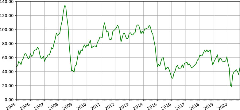
FIGURE 1. Crude oil West Texas Intermediate (WTI), January 2005–December 2020.
In recent literatures, most of the existing methods focus on the point-valued crude oil closing prices (Abramson and Finizza, 1995; Zhang et al., 2008; Kilian, 2009; Zhang et al., 2009; Shin et al., 2013; Zhao et al., 2017; Binder et al., 2018; Álvarez-Díaz, 2019). However, the use of closing prices has the disadvantage that it does not take into account the oil price variation information within a given period time, e.g., the midpoint and range of crude oil prices in October 2008 are about
Such forecasts with point-valued crude oil price data have not been particularly successful when compared with the interval-valued time series forecasts (see Sun et al., 2019). What is more, recent studies also provide empirical evidence suggesting that ITS models have achieved great success on improving the forecast accuracy in a wide range of fields such as stock price forecasting (Maia and de Carvalho, 2011; Xiong et al., 2017) and forecasting in energy markets, such as electric power demand (García-Ascanio and Maté, 2010; Hu et al., 2015), and crude oil prices (Yang et al., 2016). By accessing more information (e.g., highs, lows, midpoints, and range), an interval-based method is expected to be superior to the point-based method (Sun et al., 2018). Here, highs and lows are points of inflection for prices. The price range is the difference between two boundaries, which gives the interval length. It can be regarded as a measure of volatility to reflect the price fluctuation. For example, instead of traditional point-based method, Yang et al. (2012) introduce interval dummy variables in the autoregressive conditional interval models. Sun et al. (2019) apply a threshold autoregressive interval-valued model. Qiao et al. (2019) develop an interval-valued factor pricing model. Conclusions from prior studies suggest that interval-valued time series (ITS) models may produce more accurate forecasts.
Therefore, the desirable characteristics of the interval modeling make them ideal candidates for the prediction of crude oil prices. In addition, it is well known that a large set of factors are responsible for changes in the crude oil price, including overall economic conditions, demand and supply, monetary policy, as well as speculative trading (Hamilton, 2008; Yoshino and Taghizadeh-Hesary, 2014). Thus, the number of potential predictors can be very large. In such cases, interval-valued variable selection is considered necessary and becomes the critical step in achieving promising forecasting performances in data-rich environments. On the other hand, in practice, when only some of the variables are selected to include as the predictors in a model, model misspecification is unavoidable, which can worsen the model forecast performance of the model. Therefore, model averaging is considered to take a weighted average of possible combinations of selected interval-valued predictors.
For these reasons, this paper proposes a new two-stage procedure for interval valued crude oil price forecasting based on boosting and model averaging. First, we extend the
Next, we extend the LsoMA method developed by Liao et al. (2019) to average predictions from interval models with interval-valued exogenous variables to reduce model uncertainty. The idea of model averaging (MA) is first introduced to combine predictions from many forecasting models by Bates and Granger (1969) and has received great interest in econometrics and statistics. Model averaging is an extension of model selection which can substantially reduce the selection bias induced by selecting only one candidate model. Hoeting et al. (1999) provide a comprehensive summary of previous research on Bayesian model averaging (BMA) where models are weighted by the posterior model probabilities. Unlike BMA, frequentist model averaging (FMA) usually select the optimal weighting with the smallest information criteria scores (Buckland et al., 1997; Hjort and Claeskens, 2003; Hjort and Claeskens, 2006; Zhang and Liang, 2011; Zhang et al., 2012; Xu et al., 2014), Mallows model averaging (MMA) by Hansen (2007), jackknife model averaging (JMA) by Hansen and Racine (2012). Liao and Tsay (2016) extend MMA to the situation of the VAR models.
Univariate and bivariate methods are broadly the two main approaches in the interval modeling literature. In the univariate method, models are presented separately for a pair of attributes of interval variables (e.g., midpoint and range). The two attributes are estimated separately (De Carvalho et al., 2004; Maia et al., 2008), thus only information of one attribute is used in estimating model parameters at a time. Unlike the univariate method, the bivariate method estimates the two attributes simultaneously (e.g., Cheung et al., 2009; He et al., 2010; Lima Neto and De Carvalho, 2010; Arroyo et al., 2011; González-Rivera and Lin, 2013), which is more desirable in ITS forecasting. Therefore, in this paper, in order to consider possible interdependence between midpoint and range, the LsoMA methods are constructed following the bivariate modeling approach to efficiently use the contained information.
This paper proposes a two-stage vector boosting model averaging (2SVBMA) forecasting framework: Stage 1 uses vector
Our proposed 2SVBMA forecasting procedure has a few appealing features. First, this approach extends the forecasting success of point-valued data models of crude oil price to interval-valued data models, which is capable of assessing and forecasting the changes in both the trend and volatility of crude oil prices simultaneously due to the informational gain from interval-valued data. Second, our vector boosting method provides a parsimony and feasible solution to the interval-valued variable selection problem for interval models. Third, the extended interval-valued LsoMA model with interval-valued exogenous variables demonstrates the gains in forecast accuracy through forecast combination. By doing so, our approach improves crude oil price forecasting performances significantly.
The remainder of this paper is organized as follows. Section 2 first proposes 2SVBMA methodology, starts with extended
2 Methodology
2.1 Model Framework
Let
where
In matrix form, (1) is represented by
and
where
The least squares estimators of
and
2.2 First Stage: Vector Boosting
We first extend
Vector
1. When
2. For each step.
1) Compute the “current interval-valued residual,”
2) Regress the current interval-valued residual
The interval-valued variables that has the minimum sum of squared residuals is picked up, such that
3) The weak learner is
where
4) The strong learner
with
To avoid overfitting, a version of AIC is used to choose the optimal number of iteration
The strong learner at each step
AIC is given as
where
2.3 Second Stage: LsoMA
After selecting these important exogenous interval-valued variables, LsoMA technique is extended to interval candidate models with interval-valued exogenous variables, which is adopted to reduce model uncertainty and increase forecast accuracy.
Consider
where
where
Let the weight vector
However, this loss is infeasible because of the unknown conditional mean
where
and thus the model averaging estimator is
This shows that the squared error loss obtained from the selected weight vector
3 Empirical Implementations
This section applies the proposed 2SVBMA procedure to forecast the real price of crude oil. Data and preliminary analysis are introduced in Section 3.1. Then the selected interval-valued factors are introduced in Section 3.2. Section 3.3 introduces the candidate models. Section 3.4 provides competing methods.
3.1 Data and Preliminary Analysis
Following Wang et al. (2017), Chai et al. (2018) and Yu et al. (2019), the daily point-valued WTI crude oil prices are used to construct the interval-valued monthly prices.
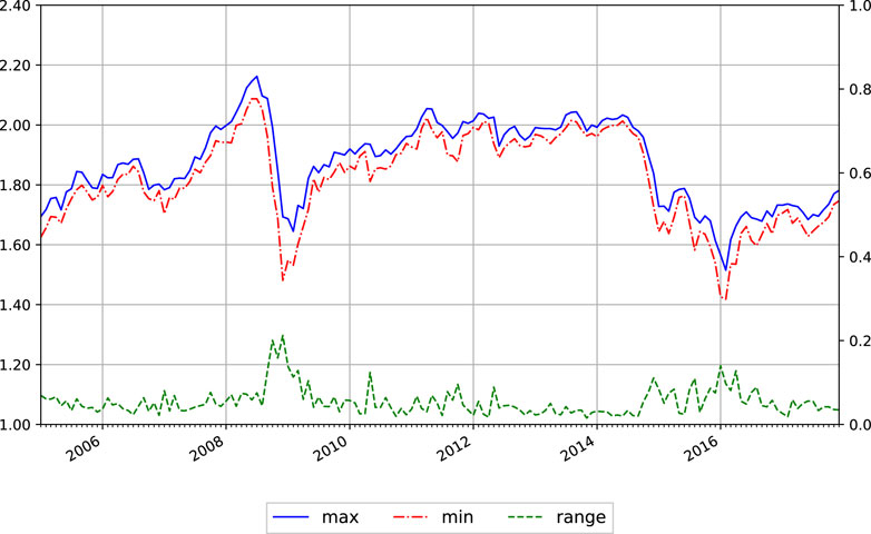
FIGURE 2. Interval valued crude oil prices from EIA, January 2005–December 2017.
Table 1 presents the summary of statistical characteristics. First, it is shown that the spread of ranges is slightly smaller than the volatility in the boundaries (

TABLE 1. Basic statistical analysis on monthly interval-valued crude oil prices.
3.2 Interval-Valued Control Variables in the First Stage
The potential choices of monthly interval-valued explanatory variables from various aspects are considered in this section, including the stock market, commodity market, technology factor, search query data, speculation, monetary market and currency market (Pan et al., 2014; Wang et al., 2016; Wang et al., 2017; Chai et al., 2018; Yu et al., 2019); see Table 2 for more discussions. First, the Augmented Dickey-Fuller tests suggest that the null hypothesis for the original control variables is hardly rejected at the 5% significance level, except for non-commercial net long ratio (
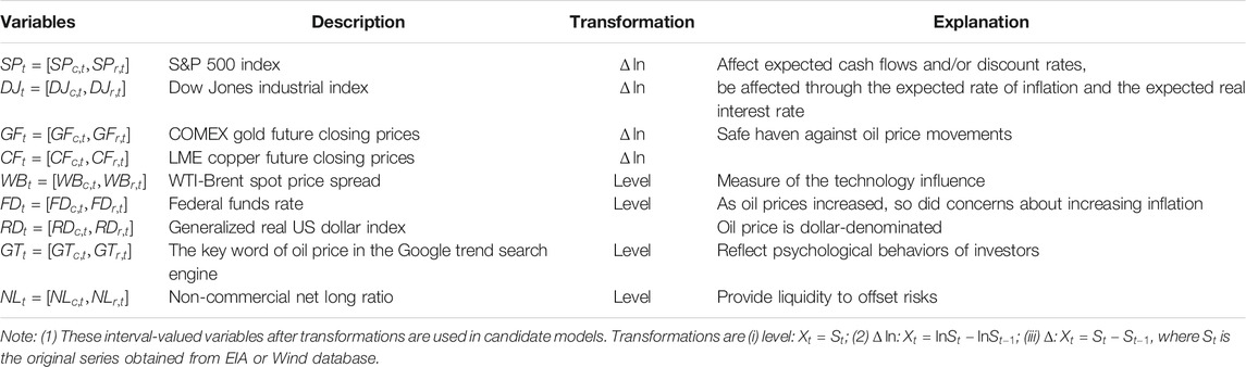
TABLE 2. Monthly interval-valued exogenous variables.
Second, Table 3 provides a summary of statistical characteristics. It is shown that no matter whether the time series is transferred by Hukuhara’s difference, the midpoints and ranges for interval-valued control variables appear to have different skewness and leptokurtic kurtosis properties. This suggests that using one attribute of ITS contains partial information only. Thus, it is highly desirable to utilize the information contained in interval-valued data.
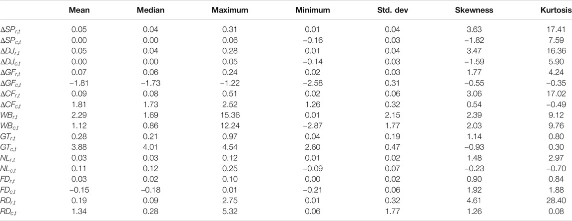
TABLE 3. Basic statistical analysis on monthly interval-valued explanatory variables.
Third, we use the extended
Furthermore, these selected interval-valued control variables have important economic interpretation for crude oil prices as follows:
3.3 Model Averaging in the Second Stage
3.3.1 Candidate Models
We consider 6 lagged dependent variables
Model 1.
Model 2.
Model 3.
Model 4.
Model 5.
Model 6.
Next, 6 exogenous variables are added to Model 6 to construct Models 7–12, sorted by relevance to
Model 7.
Model 8.
Model 9.
Model 10.
Model 11.
Model 12.
These candidate models are used for LsoMA in the second stage. We do
3.4 Competing Methods
In this paper, we compare 2SVBMA forecasts with various competing methods, including AIC, BIC, HQ, Mallows model averaging (MMA; Liao et al., 2019), smoothed AIC (SAIC), smoothed BIC (SBIC) and smoothed Hannan-Quinn (SHQ) based on the same set of candidate models (model 1 - model 12).
The AIC criterion for the
Four model averaging (or forecast combination) methods are considered here. MMA proposed by Liao and Tsay (2016) is an extension of Mallows criterion to vector regression models. Specifically, the multivariate Mallow criterion for model averaging takes the following form:
where
SAIC, SBIC and SHQ are simple model averaging methods with the weights
and
and
respectively.
4 Empirical Results
This section compares the forecasting performance of the proposed 2SVBMA approach with various competing methods presented in previous studies by using interval-valued crude oil prices. The whole sample from 2005 January to 2017 December are divided into two parts: one is used for parameter estimation, and the other is used for out-of-sample forecasting. Various subsamples for estimation and forecast are used to test prediction accuracy; see Tables 4, 5.
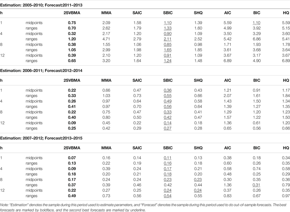
TABLE 4. MSPE (
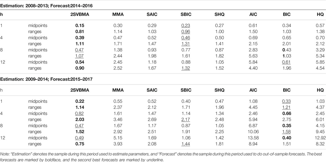
TABLE 5. MSPE (
Tables 4, 5 report the MSPEs of
Second, the SBIC estimators always produce the second-best forecasts after the 2SVBMA estimator among all model averaging methods, while SAIC achieves higher forecast criteria than other model averaging methods. Similarly, BIC always yields best forecasts among all model selection methods, while the AIC estimator achieves higher MSFE in most cases. This happens because AIC prefers selecting the relatively complicated model, which is inappropriate for out-of-sample forecasting even though it has good in-sample fitting. A simple model may be better for out-of-sample forecasting.
Furthermore, it is shown that at the second stage, model averaging forecasts outperform model selection forecasts in almost 90% of all cases. The significant advantages of model averaging support the argument of Rapach et al. (2010) that “model uncertainty and instability seriously impair the forecasting ability of individual predictive regression models.”
Overall, the proposed approach using interval-valued data is capable of assessing and forecasting the changes in both level and volatility. We can see from the results that forecasting with model averaging is generally better than obtaining the predictions from just one model (model selection). Since we may choose a very different model when there are small changes in the original data set, which may lead to a big change in the final conclusions, resulting in non-effective decision-making due to the unstable forecasting process. The proposed method is able to help obtain more stable decision-making when a long list of interval-valued predictors is available in a wide range of fields, for example, the daily trading strategy in the finance field.
5 Conclusion
We propose a novel 2SVBMA forecasting procedure to capture the relevant information available in the interval format and the underlying characteristics of crude oil price movements. Vector
There are some limitations and potential extensions of our study. First, more advanced optimization algorithms for interval-valued variable selection can be proposed in future work. Second, the candidate models with different structures in model averaging methods can further be developed to enhance forecasting. It would also be interesting to develop interval-based machine learning methods to improve forecast accuracy. Furthermore, the proposed methodology in this paper can be extended to the vector autoregressive (VAR) model, which can cover more applications in economics and finance.
In general, 2SVBMA provides a methodological framework for interval-valued data forecasting when there are a large number of potential predictors. For example, this methodology can be used to quantify the impact of COVID-19 pandemic on oil and gas industry. 2SVBMA can also provide implications for the post-COVID recovery management. The accurate prediction of crude oil prices will assist policy makers in understanding issues affecting different oil industry segments, and help governments be better prepared for the recovery.
6 Compliance With Ethical Standards
The authors thank a number of the participants at Symposium on Interval Data Modelling: Theory and Applications (SIDM 2019) in Beijing for their valuable comments and suggestions. This work was partially supported by National Natural Science Foundation of China (Nos. 71973116, 71988101, 72073126, 72091212), and the disciplinary funding of Central University of Finance and Economics. The authors declare no competing interests. This article does not contain any studies with human participants performed by any of the authors.
Data Availability Statement
The original contributions presented in the study are included in the article/Supplementary Material, further inquiries can be directed to the corresponding author.
Author Contributions
All three authors contributed equally to this work and the order of authorship has nothing other than alphabetical significance.
Funding
This work was partially supported by National Natural Science Foundation of China (Nos. 71973116, 71988101, 72073126, 72091212), the funding of Forecasting and Monitoring of COVID-19 in countries along "Belt and Road" and Related Economic Impacts (ANSO-SBA-2020-12), and the disciplinary funding of Central University of Finance and Economics.
Conflict of Interest
The authors declare that the research was conducted in the absence of any commercial or financial relationships that could be construed as a potential conflict of interest.
Publisher’s Note
All claims expressed in this article are solely those of the authors and do not necessarily represent those of their affiliated organizations, or those of the publisher, the editors and the reviewers. Any product that may be evaluated in this article, or claim that may be made by its manufacturer, is not guaranteed or endorsed by the publisher.
References
Abramson, B., and Finizza, A. (1995). Probabilistic Forecasts from Probabilistic Models: a Case Study in the Oil Market. Int. J. Forecast. 11, 63–72. doi:10.1016/0169-2070(94)02004-9
Álvarez-Díaz, M. (2019). Is it Possible to Accurately Forecast the Evolution of Brent Crude Oil Prices? an Answer Based on Parametric and Nonparametric Forecasting Methods. Empirical Econ. 59, 1285–1305. doi:10.1007/s00181-019-01665-w
Arroyo, J., González-Rivera, G., and Maté, C. (2011). “Forecasting with Interval and Histogram Data: Some Financial Applications,” in Handbook of Empirical Economics and Finance. Editors A. Ullah, and D. E. A. Giles (New York: Chapman & Hall), 247–279.
Balcilar, M., Gupta, R., and Miller, S. M. (2015). Regime Switching Model of Us Crude Oil and Stock Market Prices: 1859 to 2013. Energ. Econ. 49, 317–327. doi:10.1016/j.eneco.2015.01.026
Bates, J. M., and Granger, C. W. J. (1969). The Combination of Forecasts. Or 20, 451–468. doi:10.2307/3008764
Baur, D. G., and Lucey, B. M. (2010). Is Gold a Hedge or a Safe haven? an Analysis of Stocks, Bonds and Gold. Financial Rev. 45, 217–229. doi:10.1111/j.1540-6288.2010.00244.x
Binder, K. E., Pourahmadi, M., and Mjelde, J. W. (2018). The Role of Temporal Dependence in Factor Selection and Forecasting Oil Prices. Empirical Econ. 58, 1–39. doi:10.1007/s00181-018-1574-9
Buckland, S. T., Burnham, K. P., and Augustin, N. H. (1997). Model Selection: An Integral Part of Inference. Biometrics 53, 603–618. doi:10.2307/2533961
Buhlmann, P. (2006). Boosting for High-Dimensional Linear Models. Ann. Stat. 34, 559–583. doi:10.1214/009053606000000092
Chai, J., Xing, L.-M., Zhou, X.-Y., Zhang, Z. G., and Li, J.-X. (2018). Forecasting the Wti Crude Oil price by a Hybrid-Refined Method. Energ. Econ. 71, 114–127. doi:10.1016/j.eneco.2018.02.004
Cheung, Y.-L., Cheung, Y.-W., and Wan, A. T. K. (2009). A High-Low Model of Daily Stock price Ranges. J. Forecast. 28, 103–119. doi:10.1002/for.1087
De Carvalho, F. A. T., Lima Neto, E. A., and Tenorio, C. P. (2004). “A New Method to Fit a Linear Regression Model for Interval-Valued Data,” in Lecture Notes in Computer Science, K12004 Advances in Artificial Intelligence (Berlin: Springer-Verlag).
Ding, H., Kim, H.-G., and Park, S. Y. (2016). Crude Oil and Stock Markets: Causal Relationships in Tails? Energ. Econ. 59, 58–69. doi:10.1016/j.eneco.2016.07.013
Donald, S. G., Imbens, G. W., and Newey, W. K. (2009). Choosing Instrumental Variables in Conditional Moment Restriction Models. J. Econom. 152, 28–36. doi:10.1016/j.jeconom.2008.10.013
Ebrahim, Z., Inderwildi, O. R., and King, D. A. (2014). Macroeconomic Impacts of Oil price Volatility: Mitigation and Resilience. Front. Energ. 8, 9–24. doi:10.1007/s11708-014-0303-0
Fan, J., and Li, R. (2001). Variable Selection via Nonconcave Penalized Likelihood and its oracle Properties. J. Am. Stat. Assoc. 96, 1348–1360. doi:10.1198/016214501753382273
Fantazzini, D., and Fomichev, N. (2014). Forecasting the Real price of Oil Using Online Search Data. Ijcee 4, 4–31. doi:10.1504/ijcee.2014.060284
Frank, L. E., and Friedman, J. H. (1993). A Statistical View of Some Chemometrics Regression Tools. Technometrics 35, 109–135. doi:10.1080/00401706.1993.10485033
García-Ascanio, C., and Maté, C. (2010). Electric Power Demand Forecasting Using Interval Time Series: A Comparison between Var and Imlp. Energy Policy 38, 715–725. doi:10.1016/j.enpol.2009.10.007
González-Rivera, G., and Lin, W. (2013). Constrained Regression for Interval-Valued Data. J. Business Econ. Stat. 31, 473–490. doi:10.1080/07350015.2013.818004
Hansen, B. E. (2007). Least Squares Model Averaging. Econometrica 75, 1175–1189. doi:10.1111/j.1468-0262.2007.00785.x
Hansen, B. E., and Racine, J. S. (2012). Jackknife Model Averaging. J. Econom. 167, 38–46. doi:10.1016/j.jeconom.2011.06.019
He, A. W. W., Kwok, J. T. K., and Wan, A. T. K. (2010). An Empirical Model of Daily Highs and Lows of West texas Intermediate Crude Oil Prices. Energ. Econ. 32, 1499–1506. doi:10.1016/j.eneco.2010.07.012
Hjort, N. L., and Claeskens, G. (2006). Focused Information Criteria and Model Averaging for the Cox hazard Regression Model. J. Am. Stat. Assoc. 101, 1449–1464. doi:10.1198/016214506000000069
Hjort, N. L., and Claeskens, G. (2003). Frequentist Model Average Estimators. J. Am. Stat. Assoc. 98, 879–899. doi:10.1198/016214503000000828
Hoeting, J. A., Madigan, D., Raftery, A. E., and Volinsky, C. T. (1999). Bayesian Model Averaging: a Tutorial. Stat. Sci. 14, 382–417. doi:10.1214/ss/1009212519
Hu, Z., Bao, Y., Chiong, R., and Xiong, T. (2015). Mid-term Interval Load Forecasting Using Multi-Output Support Vector Regression with a Memetic Algorithm for Feature Selection. Energy 84, 419–431. doi:10.1016/j.energy.2015.03.054
Kang, S. H., McIver, R., and Yoon, S.-M. (2017). Dynamic Spillover Effects Among Crude Oil, Precious Metal, and Agricultural Commodity Futures Markets. Energ. Econ. 62, 19–32. doi:10.1016/j.eneco.2016.12.011
Kilian, L. (2009). Not all Oil price Shocks Are Alike: Disentangling Demand and Supply Shocks in the Crude Oil Market. Am. Econ. Rev. 99, 1053–1069. doi:10.1257/aer.99.3.1053
Knight, K., and Fu, W. (2000). Asymptotics for Lasso-type Estimators. Ann. Stat. 28, 1356–1378. doi:10.1214/aos/1015957397
Li, D., Linton, O., and Lu, Z. (2015a). A Flexible Semiparametric Forecasting Model for Time Series. J. Econom. 187, 345–357. doi:10.1016/j.jeconom.2015.02.025
Li, X., Ma, J., Wang, S., and Zhang, X. (2015b). How Does Google Search Affect Trader Positions and Crude Oil Prices? Econ. Model. 49, 162–171. doi:10.1016/j.econmod.2015.04.005
Liao, J.-C., and Tsay, W.-J. (2016). Multivariate Least Squares Forecasting Averaging by Vector Autoregressive Models. Available at SSRN 2827416.
Liao, J., Zong, X., Zhang, X., and Zou, G. (2019). Model Averaging Based on Leave-Subject-Out Cross-Validation for Vector Autoregressions. J. Econom. 209, 35–60. doi:10.1016/j.jeconom.2018.10.007
Lima Neto, E. d. A., and De Carvalho, F. d. A. T. (2010). Constrained Linear Regression Models for Symbolic Interval-Valued Variables. Comput. Stat. Data Anal. 54, 333–347. doi:10.1016/j.csda.2009.08.010
Maia, A. L. S., and de Carvalho, F. d. A. T. (2011). Holt's Exponential Smoothing and Neural Network Models for Forecasting Interval-Valued Time Series. Int. J. Forecast. 27, 740–759. doi:10.1016/j.ijforecast.2010.02.012
Maia, A. L. S., De Carvalho, F. d. A. T., and Ludermir, T. B. (2008). Forecasting Models for Interval-Valued Time Series. Neurocomputing 71, 3344–3352. doi:10.1016/j.neucom.2008.02.022
Miller, J. I., and Ratti, R. A. (2009). Crude Oil and Stock Markets: Stability, Instability, and Bubbles. Energ. Econ. 31, 559–568. doi:10.1016/j.eneco.2009.01.009
Ng, S., and Bai, J. (2009). Selecting Instrumental Variables in a Data Rich Environment. J. Time Ser. Econom. 1, 4. doi:10.2202/1941-1928.1014
Pan, Z., Wang, Y., and Yang, L. (2014). Hedging Crude Oil Using Refined Product: A Regime Switching Asymmetric Dcc Approach. Energ. Econ. 46, 472–484. doi:10.1016/j.eneco.2014.05.014
Qiao, K., Sun, Y., and Wang, S. (2019). Market Inefficiencies Associated with Pricing Oil Stocks during Shocks. Energ. Econ. 81, 661–671. doi:10.1016/j.eneco.2019.04.016
Rapach, D. E., Strauss, J. K., and Zhou, G. (2010). Out-of-sample Equity Premium Prediction: Combination Forecasts and Links to the Real Economy. Rev. Financ. Stud. 23, 821–862. doi:10.1093/rfs/hhp063
Reboredo, J. C. (2013). Is Gold a Hedge or Safe haven against Oil price Movements? Resour. Pol. 38, 130–137. doi:10.1016/j.resourpol.2013.02.003
Shin, H., Hou, T., Park, K., Park, C.-K., and Choi, S. (2013). Prediction of Movement Direction in Crude Oil Prices Based on Semi-supervised Learning. Decis. Support Syst. 55, 348–358. doi:10.1016/j.dss.2012.11.009
Souček, M. (2013). Crude Oil, Equity and Gold Futures Open Interest Co-movements. Energ. Econ. 40, 306–315. doi:10.1016/j.eneco.2013.07.010
Sun, Y., Han, A., Hong, Y., and Wang, S. (2018). Threshold Autoregressive Models for Interval-Valued Time Series Data. J. Econom. 206, 414–446. doi:10.1016/j.jeconom.2018.06.009
Sun, Y., Zhang, X., Hong, Y., and Wang, S. (2019). Asymmetric Pass-Through of Oil Prices to Gasoline Prices with Interval Time Series Modelling. Energ. Econ. 78, 165–173. doi:10.1016/j.eneco.2018.10.027
Taghizadeh-Hesary, F., Rasoulinezhad, E., and Kobayashi, Y. (2016). Oil price Fluctuations and Oil Consuming Sectors: An Empirical Analysis of Japan. Econom. Pol. Ener. Environ. (2), 33–51. doi:10.3280/EFE2016-002003
Wang, X., Zhang, Z., and Li, S. (2016). Set-valued and Interval-Valued Stationary Time Series. J. Multivariate Anal. 145, 208–223. doi:10.1016/j.jmva.2015.12.010
Wang, Y., Liu, L., and Wu, C. (2017). Forecasting the Real Prices of Crude Oil Using Forecast Combinations over Time-Varying Parameter Models. Energ. Econ. 66, 337–348. doi:10.1016/j.eneco.2017.07.007
Wu, B., Wang, L., Lv, S.-X., and Zeng, Y.-R. (2021). Effective Crude Oil price Forecasting Using New Text-Based and Big-Data-Driven Model. Measurement 168, 108468. doi:10.1016/j.measurement.2020.108468
Xiong, T., Li, C., and Bao, Y. (2017). Interval-valued Time Series Forecasting Using a Novel Hybrid Holti and Msvr Model. Econ. Model. 60, 11–23. doi:10.1016/j.econmod.2016.08.019
Xu, G., Wang, S., and Huang, J. Z. (2014). Focused Information Criterion and Model Averaging Based on Weighted Composite Quantile Regression. Scand. J. Statist 41, 365–381. doi:10.1111/sjos.12034
Yang, W., Han, A., Cai, K., and Wang, S. (2012). Acix Model with Interval Dummy Variables and its Application in Forecasting Interval-Valued Crude Oil Prices. Proced. Comp. Sci. 9, 1273–1282. doi:10.1016/j.procs.2012.04.139
Yang, W., Han, A., Hong, Y., and Wang, S. (2016). Analysis of Crisis Impact on Crude Oil Prices: a New Approach with Interval Time Series Modelling. Quantitative Finance 16, 1917–1928. doi:10.1080/14697688.2016.1211795
Yang, Y., Guo, J. e., Sun, S., and Li, Y. (2021). Forecasting Crude Oil price with a New Hybrid Approach and Multi-Source Data. Eng. Appl. Artif. Intelligence 101, 104217. doi:10.1016/j.engappai.2021.104217
Yoshino, N., and Hesary, F. T. (2014). Monetary Policy and Oil price Fluctuations Following the Subprime Mortgage Crisis. Ijmef 7, 157–174. doi:10.1504/ijmef.2014.066482
Yu, L., Zhao, Y., Tang, L., and Yang, Z. (2019). Online Big Data-Driven Oil Consumption Forecasting with Google Trends. Int. J. Forecast. 35, 213–223. doi:10.1016/j.ijforecast.2017.11.005
Zaabouti, K., Ben Mohamed, E., and Bouri, A. (2016). Does Oil price Affect the Value of Firms? Evidence from Tunisian Listed Firms. Front. Energ. 10, 1–13. doi:10.1007/s11708-016-0396-8
Zhang, X., Lai, K. K., and Wang, S.-Y. (2008). A New Approach for Crude Oil price Analysis Based on Empirical Mode Decomposition. Energ. Econ. 30, 905–918. doi:10.1016/j.eneco.2007.02.012
Zhang, X., and Liang, H. (2011). Focused Information Criterion and Model Averaging for Generalized Additive Partial Linear Models. Ann. Stat. 39, 174–200. doi:10.1214/10-aos832
Zhang, X., Wan, A. T. K., and Zhou, S. Z. (2012). Focused Information Criteria, Model Selection, and Model Averaging in a Tobit Model with a Nonzero Threshold. J. Business Econ. Stat. 30, 132–142. doi:10.1198/jbes.2011.10075
Zhang, X., Yu, L., Wang, S., and Lai, K. K. (2009). Estimating the Impact of Extreme Events on Crude Oil price: An Emd-Based Event Analysis Method. Energ. Econ. 31, 768–778. doi:10.1016/j.eneco.2009.04.003
Zhang, Y., Li, J., Liu, H., Zhao, G., Tian, Y., and Xie, K. (2020). Environmental, Social, and Economic Assessment of Energy Utilization of Crop Residue in china. Front. Energ. 15, 308–319. doi:10.1007/s11708-020-0696-x
Zhao, L., Zhang, X., Wang, S., and Xu, S. (2016). The Effects of Oil price Shocks on Output and Inflation in china. Energ. Econ. 53, 101–110. doi:10.1016/j.eneco.2014.11.017
Keywords: crude oil prices forecasting, forecast combination, interval-valued time series, model averaging, vector L2-boosting
Citation: Huang B, Sun Y and Wang S (2021) A New Two-Stage Approach with Boosting and Model Averaging for Interval-Valued Crude Oil Prices Forecasting in Uncertainty Environments. Front. Energy Res. 9:707937. doi: 10.3389/fenrg.2021.707937
Received: 12 May 2021; Accepted: 16 July 2021;
Published: 19 August 2021.
Edited by:
Farhad Taghizadeh-Hesary, Tokai University, JapanCopyright © 2021 Huang, Sun and Wang. This is an open-access article distributed under the terms of the Creative Commons Attribution License (CC BY). The use, distribution or reproduction in other forums is permitted, provided the original author(s) and the copyright owner(s) are credited and that the original publication in this journal is cited, in accordance with accepted academic practice. No use, distribution or reproduction is permitted which does not comply with these terms.
*Correspondence: Yuying Sun, c3VueXV5aW5nQGFtc3MuYWMuY24=