Ensemble Forecasting Frame Based on Deep Learning and Multi-Objective Optimization for Planning Solar Energy Management: A Case Study

There are many prediction models that have been adopted to predict uncertain and non-linear photovoltaic power time series. Nonetheless, most models neglected the validity of data preprocessing and ensemble learning strategies, which leads to low forecasting precision and low stability of photovoltaic power. To effectively enhance photovoltaic power forecasting accuracy and stability, an ensemble forecasting frame based on the data pretreatment technology, multi-objective optimization algorithm, statistical method, and deep learning methods is developed. The proposed forecasting frame successfully integrates the advantages of multiple algorithms and validly depict the linear and nonlinear characteristic of photovoltaic power time series, which is conductive to achieving accurate and stable photovoltaic power forecasting results. Three datasets of 15-min photovoltaic power output data obtained from different time periods in Belgium were employed to verify the validity of the proposed system. The simulation results prove that the proposed forecasting frame positively surpasses all comparative hybrid models, ensemble models, and classical models in terms of prediction accuracy and stabilization. For one-, two-, and three-step predictions, the MAPE values obtained from the proposed frame were less than 2, 3, and 5%, respectively. Discussion results also verify that the proposed forecasting frame is obviously different from other comparative models, and is more stable and high-efficiency. Thus, the proposed frame is highly serviceable in elevating photovoltaic power forecasting performance and can be used as an efficient instrument for intelligent grid programming.

1 Introduction

The exhaustion of fossil energy and global warming have been inescapable events for humans (Das et al., 2015; Takilalte et al., 2019; Irfan et al., 2021). To work out these events, exploring and exploiting renewable energy worldwide should be the ultimate focus of attention (Islam, 2017; Shezan et al., 2017; Liu et al., 2020; Elavarasan et al., 2021). Photovoltaic (PV) power, which is unlimited, green, and available, has become a key point in new energy resource research (Jithin and Roykumar, 2018; Shelat et al., 2019; Zhu and Pi, 2020; Tan et al., 2021). The International Energy Agency announced that, until 2019, the global accumulative installed capacity of PV power exceeded 627 GW.¹ Nevertheless, PV power is labile and fluctuates at high frequency, which unpredictably impacts the facility wastage and grid stability of the intelligent electric system. Therefore, enhancing the forecasting accuracy and stability of PV power must be considered to help solve the aforementioned tasks and optimize the intelligent electric system operation.

By reviewing past studies, we can see that several forecasting models have been proposed and developed to enhance prediction precision and effectiveness (Yildiz and Acikgoz, 2021). With respect to the calculative mechanism, the forecasting model can be summarized as the following rough categories (Abdel-Nasser and Mahmoud, 2019; Liu et al., 2022): physical, statistical, and artificial intelligent models. Physical models rely on sky cameras and satellite data to forecast PV power (Dong et al., 2020). PV power prediction with satellite imaging or sky cameras has been developed as a key theme based on data capture and cloud movement (Elsinga and van Sark, 2017). Physical methods exhibit satisfactory performance when the state of the weather is stabilized (Li et al., 2020). In contrast to physical models, statistical models use sufficient actual data to conduct short-term PV power forecasting, and these models with regard to short-term forecasting surpass physical models in terms of performance (Zhang et al., 2019). The prediction performance of statistical models is impacted when the input variables have a nonlinear relationship. Autoregressive moving average (ARMA) (David et al., 2016), autoregressive integrated moving average (ARIMA) (Pedro and Coimbra, 2012), Kalman filter (Soubdhan et al., 2016), and other statistical models have been adopted and gained significant prediction results. In addition, artificial intelligent models, which incorporate artificial neural networks (ANNs) (Yacef et al., 2014), fuzzy logic methods (Tanaka et al., 2011), and deep learning methods (DLMs) (Jiang et al., 2020), are widely adopted tools for short-term PV power forecasting (Yagli et al., 2019; Devaraj et al., 2021). Based on their outstanding capabilities, DLMs can deal with the fuzzy relationship between the actual data and forecasting data. As a booming branch of artificial intelligence methods, DLM has attracted wide attention in numerous fields (Zhou et al., 2020). Compared with the two models, DLMs depend on historical data and have high fault tolerance, which means that DLMs can robustly and adaptively predict PV power. In addition, DLMs can dispose of nonlinear data, conduct adaptive forecasting, and judge fuzzy relationships (Li, 2020). Nonetheless, DLMs have instinctive shortcomings, including over-fitting, easy to local optimum, and low convergence speed (Jiang and Liu, 2019). Apart from the abovementioned forecasting models, hybrid models have also received great attention. Hybrid approaches can overcome the limitation of individual model by combining predictor with other algorithms (Kushwaha and Pindoriya, 2019). For example, Qu et al. (2021b) established a hybrid gated recurrent unit (GRU) to forecast day-ahead PV generation and proved hybrid GRU is superior to individual GRU in terms of forecasting accuracy. Korkmaz (2021) used variational mode decomposition approach and convolutional neural network (CNN) to improve PV power forecasting ability. Relative to benchmark deep learning models, the proposed hybrid model can provide better forecasting results. Eseye et al. (2018) developed a novel hybrid short-term forecasting method, which integrated wavelet transform (WT), particle swarm optimization (PSO) with support vector machine (SVM) to enhance PV power forecasting precision. By comparing with various prediction approaches, the proposed model showed excellent prediction performance, which is helpful to integrate PV into power grid. However, forecasting performance of a definite forecasting model is different with respect to different datasets and observation sites. Thus, one forecasting approach cannot be applied to all forecasting situations.

The drawbacks of the aforementioned methods can be concluded as follows:

(1) Physical models cannot obtain satisfactory results pertaining to short-term PV power prediction based on several disadvantages: running efficiency is lower, consumed computing resources are expensive, and forecasting results are unsatisfactory. Hence, physical models cannot offer a satisfactory service for short-term PV power forecasting.

(2) Statistical models are poor in predicting data with high fluctuation and nonlinear characteristics. It cannot effectively forecast PV power based on the linear hypothesis (Niu and Wang, 2019).

(3) Compared with the aforementioned models, the artificial intelligence model, such as DLMs, can detect the nonlinear relationship between the historical and forecasted values. It has attracted several researchers over the past several years for the validity to forecast complicated relationships (Feng et al., 2017). Nonetheless, DLMs have instinctive shortcomings, such as over-fitting, easy to local optimum, and low convergence speed (Iversen et al., 2016).

(4) Because of the instinctive drawbacks of each model, the individual model cannot forecast time-series data that vary under the changing environment, resulting in poor forecasting performance in some situations.

To overcome the above disadvantages, the ensemble learning strategy based on multiple forecasting models that proposed by Bates and Granger (1969) has been widely used by researchers. Ensemble strategy employs multiple forecasting models to achieve an aggregated result that is superior to every base forecasting model (Opitz and Maclin, 1999). The main principle of this strategy is to obtain optimal weights to ensure the minimum sum of squared errors of the training set (Hao and Tian, 2019). By combing multiple predictors, we can better utilize more useful information and remove particular deviations brought by individual predictor. Moreover, the ensemble strategy can successfully integrate the merit of all involved sub-predictors, such as their good ability to grasp different data characteristic and the good property to overcome negative effect (e.g., overfitting), which is proved to be effective to improve forecasting performance in many forecasting fields (Xiao et al., 2015; Liu et al., 2019; Wang et al., 2021). Yang and Dong (2018) proposed a seasonal time series ensemble model that used six component models from different families and 8 ensemble methods to conduct PV power output forecasting. A simple remedy was added to the ensemble model, which was proved to be effective to improve forecasting ability. Li et al. (2020) used wavelet packet decomposition (WPD) to decompose PV power data and used long short-term memory (LSTM) to forecast the decomposed series. The predicted sub-series are ultimately integrated based on linear weighting strategy to obtain the final forecasting values. Simulation results verified its high-quality forecasting ability. Sharma et al. (2021) proposed a novel forecasting frame, where the maximal overlap discrete wavelet transform technique was used for decomposition and the LSTM was used for sub-series forecasting. By integrating the sub-series forecasting results, the final PV power forecasting results were finally obtained. More studies about ensemble forecasting models are listed in Table 1. From the above review, we can find that most existing ensemble models are more likely to use a single forecasting model. However, PV power series is fluctuant and uncertain with both intricate linear and nonlinear characteristics, which must be captured by different class of forecasting models. To this end, in this paper, both statistical model and DLMs are combined together to better grasp the linear and nonlinear characteristics of PV power series. Moreover, some existing ensemble models use linear weighting method to calculate the final ensemble forecasting results. Considering linear weighting method may not reflect the importance of the prediction results of each component, a multi-objective optimization algorithm (MOOA) is used to optimize the combining weights, which can effectively improve PV power forecasting performance. Besides, data preprocessing is an important process in PV power forecasting because it can filter the high-frequency noise in original time series and retain the useful information. Nevertheless, most studies may ignore the importance of data preprocessing or adopt poor preprocessing methods. In this paper, an effective data preprocessing method, namely singular spectrum analysis (SSA), is used to preprocess the historical PV power output forecasting, which can better grasp the data characteristic of PV power series and effectively improve forecasting ability.

TABLE 1

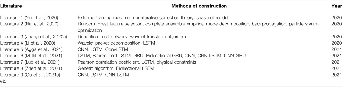
TABLE 1. Relevant studies.

In our study, proposed ensemble forecasting frame (PEFF) is built, which incorporates SSA, multi-objective grasshopper algorithm (MOGOA), ARIMA, and DLMs. Specifically, SSA was selected to eliminate irregular fluctuations of observed values in a complex environment. SSA can effectively process the original time series to enhance the forecasting performance. ARIMA and three DLMs (i.e., deep belief network (DBN), GRU, LSTM) were adopted to conduct PV power forecasting, and the ensemble coefficient of each model was obtained using MOGOA. ARIMA can effectively predict the linear trend of PV power generation, whereas DLMs can effectively predict nonlinear trends. The PEFF fills the gap between the statistical and artificial intelligence models. MOGOA can effectively combine forecasting results based on an effective style. The PEFF that integrates the benefits of individual models with data pretreatment techniques and intelligent optimization algorithms can validly improve the PV power prediction ability (Tian and Hao, 2018).

The leading course of our study relative to other studies in the domain of PV power forecasting is summarized below:

(1) A data pretreatment technique was adopted to relieve the random fluctuation of PV power sequences in real time. The observed PV power output time series will be disintegrated into several subseries; then, the subseries with the highest frequency fluctuation is abnegated, and the residuals are structured to conduct PV power forecasting. Considering this disposal, the essential character of PV power could be better extracted, and hence, the forecasting performance can be greatly improved.

(2) The statistical model is beneficial to grasp linear characteristics, while DLMs make for nonlinear characteristics. For the sake of comprehensive control of the linear and nonlinear characteristics of PV power, ARIMA (the statistical model) is used to forecast the linear trend, and three DLMs are used for the nonlinear trends.

(3) MOGOA, as an effective parameter optimization technology, can determine the optimal coefficient of each sub-model. MOGOA with an archive to determine approximative values of the Pareto optimal solution can prompt prediction precision and prediction stability. MOGOA can help deal with an intricate optimization problem.

(4) The developed ensemble frame (EF) can assist in the operation and optimization of smart grids. Based on the realistic PV power data and comprehensive prediction result analyses, the PEFF is verified as an effective forecasting frame and can be applied to other forecasting fields in future.

At present, an accurate and stable forecasting system is urgently needed for renewable energy generation. However, in the current study, the developed prediction models have defects. Therefore, we propose a PEFF for PV power generation prediction to compensate for the defects of the current prediction model and provide a new scheme for PV power generation prediction.

2 Methods

In this section, SSA and MOGOA are presented in detail, and a particular process of the PEFF is introduced.

2.1 Data Preprocessing Strategy

SSA, as an instrumental data preprocessing technique to process the observed PV power values, has been continually adopted in various fields, such as biology (Hassani and Ghodsi, 2015), physics (Krishnannair et al., 2016), climatology (Unnikrishnan and Jothiprakash, 2018), and economics (de Carvalho and Rua, 2017). The flow of the SSA is listed as follows:

Step 1. Embedding

Conversing original time series $\mathrm{X}=\left({\mathit{x}}_{\mathit{1}}\mathrm{,}{\mathit{x}}_{\mathit{2}},\cdots {\mathit{x}}_{\mathit{N}}\right)$ into $\mathrm{Z}=\left({\mathit{z}}_{\mathit{1}}\mathrm{,}{\mathit{z}}_{\mathit{2}}\mathrm{,}\cdots \mathrm{,}{\mathit{z}}_{\mathit{K}}\right)$ as Eq. 1.

$\mathrm{X}=\left({\mathit{x}}_{\mathit{1}}\mathit{,}{\mathit{x}}_{\mathit{2}}\mathrm{,}\cdots \mathrm{,}{\mathit{x}}_{\mathit{N}}\right)\to \mathrm{Z}=\left({\mathit{z}}_{\mathit{1}}\mathrm{,}{\mathit{z}}_{\mathit{2}}\mathrm{,}\cdots \mathrm{,}{\mathit{z}}_{\mathit{K}}\right),(1)$

where ${\mathit{z}}_{\mathit{i}}={\left({\mathit{x}}_{\mathrm{i}}\mathrm{,}{\mathit{x}}_{\mathit{i+1}}\mathrm{,}\cdot \cdot \cdot \mathrm{,}{\mathit{x}}_{\mathit{i+L-1}}\right)}^{\mathrm{T}}\in {\mathit{R}}^{\mathit{L}},\mathit{K=}\mathit{N-}\mathit{L+1}$, $\mathit{L}\in \mathit{[2,N]}$. The consequence of this mapping is embodied as a trajectory matrix with the mathematical expression of

$\mathbf{Z}=\left[{\mathbf{Z}}_1,{\mathbf{Z}}_{\mathrm{2}},\cdot \cdot \cdot ,{\mathit{Z}}_{\mathit{K}}\right]={\left({\mathbf{z}}_{\mathit{ij}}\right)}_{\mathit{i,}\mathit{j=1}}^{\mathit{L,}\mathit{K}}=\left(\begin{array}{cccc}{\mathit{x}}_{\mathrm{1}}& {\mathit{x}}_{\mathrm{2}}& \cdot \cdot \cdot & {\mathit{x}}_{\mathit{K}}\\ {\mathit{x}}_{\mathrm{2}}& {\mathit{x}}_{\mathrm{3}}& \cdot \cdot \cdot & {\mathit{x}}_{\mathit{K+1}}\\ \cdot \cdot \cdot & \cdot \cdot \cdot & \cdot \cdot \cdot & \cdot \cdot \cdot \\ {\mathit{x}}_{\mathit{L}}& {\mathit{x}}_{\mathit{L+1}}& \cdot \cdot \cdot & {\mathit{x}}_{\mathit{N}}\end{array}\right),(2)$

Step 2. Singular values decomposition

Given a covariance matrix ($\mathbf{S}=\mathit{X}{\mathit{X}}^{\mathrm{T}}$), this step is employed to obtain L eigenvalues (${\mathrm{\lambda }}_1\mathrm{,}{\mathrm{\lambda }}_2\mathrm{,}\cdot \cdot \cdot \mathrm{,}{\mathrm{\lambda }}_{\mathit{L}}$) and eigenvectors (${\mathbf{U}}_1\mathrm{,}{\mathbf{U}}_2\mathrm{,}\cdot \cdot \cdot \mathrm{,}{\mathbf{U}}_{\mathit{L}}$). Suppose $\mathit{t}=\mathit{max}\left(\mathrm{i, such that }{\mathrm{\lambda }}_{\mathrm{\iota }}\mathrm{>0}\right)$ and ${\mathbf{V}}_{\mathit{i}}\mathrm{=}{\mathbf{X}}^{\mathbf{T}}{\mathbf{U}}_{\mathit{i}}\sqrt{{\lambda }_i}$ $\left(\mathit{i}=1\mathrm{,}2\mathrm{,}\mathrm{...}\mathrm{,t}\right)$, then, $\mathit{S}=\mathit{X}{\mathit{X}}^{\mathrm{T}}$ in this step can be indicated by

$\mathbf{Z}={\mathbf{E}}_1+{\mathbf{E}}_2+\cdot \cdot \cdot +{\mathbf{E}}_{\mathit{t}},(3)$

where ${\mathbf{E}}_{\mathit{i}}=\sqrt{{\mathrm{\lambda }}_{\mathit{i}}}{\mathbf{U}}_{\mathit{i}}{\mathbf{V}}_{\mathit{i}}$ and the rank of $Z_i$ is 1. Therefore, ${\mathbf{V}}_{\mathrm{1}}\mathrm{,}{\mathbf{V}}_{\mathrm{2}}\mathrm{,}\cdot \cdot \cdot \mathrm{,}{\mathbf{V}}_{\mathrm{t}}$ are the principal components, and $\left(\sqrt{{\mathrm{\lambda }}_{\mathit{i}}},{\mathbf{U}}_{\mathit{i}},{\mathbf{V}}_{\mathit{i}}\right)$ denotes the characteristic root of the trajectory matrix (Z).

Step 3. Grouping

The interval $\left(\mathrm{i}=1\mathrm{,}2\mathrm{,}\mathrm{...}\mathrm{,t}\right)$ is disintegrated into several components ($S_1\mathrm{,}{S}_2\mathrm{,}\cdot \cdot \cdot \mathrm{,}{S}_{\mathrm{m}}$) without a connection between them. Suppose that $\mathbf{S}=\left({\mathrm{s}}_{\mathrm{1}}\mathrm{,}{\mathrm{s}}_{\mathrm{2}}\mathrm{,}\cdot \cdot \cdot \mathrm{,}{\mathrm{s}}_{\mathrm{p}}\right)$, then ${\mathbf{Z}}_{\mathit{S}}$ is defined as ${\mathbf{Z}}_{\mathit{S}}={\mathbf{Z}}_{{\mathit{s}}_{\mathit{1}}}+{\mathbf{Z}}_{{\mathit{s}}_{\mathrm{2}}}+\cdot \cdot \cdot +{\mathbf{Z}}_{{\mathit{s}}_{\mathit{p}}}$, and Z can be disintegrated into $\mathbf{Z}={\mathbf{Z}}_{{\mathit{S}}_{\mathit{1}}}+{\mathbf{Z}}_{{\mathit{S}}_{\mathit{2}}}+\cdot \cdot \cdot +{\mathbf{Z}}_{{\mathit{S}}_{\mathit{m}}}$.

Step 4. Diagonal averaging

In this step, the grouping result is converted into a sequence with N points. Assume that Z is an L $\ast$ K matrix, ${\mathit{L}}^{\ast }=\min \left(\mathrm{L,K}\right)$ and ${\mathit{K}}^{\ast }=\max \left(\mathrm{L,K}\right)$. If L < K, then ${\mathrm{z}}_{\mathrm{ij}}^{\mathrm{*}}\mathrm{=}{\mathrm{z}}_{\mathrm{ij}}$, or else, ${\mathrm{z}}_{\mathrm{ij}}^{\mathrm{*}}\mathrm{=}{\mathrm{z}}_{\mathrm{ji}}$. Finally, Z is turned into a sequence $\left(r_{\mathrm{1}}\mathrm{,}{r}_{\mathrm{2}}\mathrm{,}\cdots \mathrm{,}{r}_{\mathit{N}}\right)$ based on the following formula:

$r_k=\{\begin{array}{c}\frac{1}{k+1}{\displaystyle {\sum }_{q=1}^{k+1}{z}_{\mathit{q,k-q+1}}^{\ast },\mathbf{1}\le k\le L^{\text{*}}}\\ \frac{1}{L^{\ast }}{\displaystyle {\sum }_{q=1}^{L^{\ast }}{Z}_{q,k-q+1}^{\ast }L\text{*}\le k\le K^{\text{*}}}\\ \frac{1}{N-K+1}{\displaystyle {\sum }_{q=1}^{N-K^{\ast }+1}{Z}_{\mathrm{q,k-q+}1}^{\ast }{K}^{\text{*}}\le k\le N}\end{array},(4)$

2.2 Intelligent Optimization Algorithm

MOGOA simulates the location of the grasshopper population, which is used to search for the optimal solution to a definite problem. Based on related articles (Mirjalili et al., 2018), the operating mechanism of the MOGOA can be summarized as follows:

The motion of each grasshopper is principally influenced by individual interactions, weight, and wind strength. In addition, ${\mathit{X}}_{\mathit{i}}$ represents the location of the ith grasshopper, as shown in Eq. 5.

$X_i=S_i+G_i+A_i,(5)$

where $S_i$, $G_i$, and $A_i$ denote the individual interaction, weight, and wind strength of each grasshopper, respectively.

$S_i$ can be quantized by subsequent equations:

$S_i={\displaystyle \sum _{\begin{array}{l}j=1\\ j\ne i\end{array}}^{N}s\left(d_{ij}\right)}{\widehat{d}}_{ij},(6)$

$d_{ij}=\left|X_j-X_i\right|,(7)$

${\widehat{d}}_{ij}=\left(X_j-X_i\right)/d_{ij},\mathrm{and}(8)$

$\mathit{s}\left(r\right)=f{\mathbf{e}}^{-r/l}-{\mathbf{e}}^{-r},(9)$

where $d_{ij}$ denotes the space between the ith and jth grasshopper and ${\widehat{d}}_{ij}$ denotes a normalized vector from the ith grasshopper to the jth grasshopper. $\mathit{s}\left(r\right)$ quantizes individual interactions based on f and l.

The weight is computed via Eq. 10:

$G_i=-\mathit{g}{\widehat{\mathbf{e}}}_g,(10)$

Here, g denotes the gravitational coefficient, and ${\widehat{\mathbf{e}}}_g$ defines a normalized vector to the earth’s core. In addition, the wind strength of each grasshopper can be calculated using Eq. 11.

$A_i=\mathit{u}{\widehat{\mathbf{e}}}_w,(11)$

Here, u defines a constant parameter, and ${\widehat{\mathbf{e}}}_w$ denotes a vector normalized to wind direction. Moreover, Eq. 5 can be expressed in detail using Eq. 12.

$X_i={\displaystyle \sum _{\begin{array}{l}j=1\\ j\ne i\end{array}}^N\mathit{s}\left(\left|X_j-X_i\right|\right)\frac{X_j-X_i}{d_{ij}}-g{\widehat{\mathbf{e}}}_g+u{\widehat{\mathbf{e}}}_w},(12)$

Here, N denotes population size. Moreover, the aforementioned formulas simulate the motion of the ith grasshopper under hypothetical status.

The force applied by gravitation is insignificant. The wind strength is related to the orientation (${\widehat{T}}_d$). Therefore, X_i can be extended as follows:

$X_i^d=\mathbf{c}\left({\displaystyle \sum _{\begin{array}{l}j=1\\ j\ne i\end{array}}^N\mathbf{c}\frac{u{b}_d-l{b}_d}{2}s\left(\left|X_j^d-X_i^d\right|\right)}\frac{X_j-X_i}{d_{ij}}\right)+{\widehat{T}}_d,(13)$

Here, ub_d and lb_d represent the upper and lower boundaries of the dth variable, respectively. ${\widehat{\mathit{T}}}_d$ denotes the dth variable value of the optimal solution. In addition, c determined using Eq. 14 can reduce exploration and improve exploitation such that the operation speed can be correspondingly decreased based on the iteration number.

$\mathbf{c}=c_{max}-l\frac{c_{max}-c_{min}}{L},(14)$

Here, $c_{max}$ and $c_{min}$ denote the maximum and minimum values, respectively, and l and L represent the present iteration and max iteration, respectively.

To conduct multi-objective optimization via GOA, a Pareto optimal solution is adopted to modify the solution distribution. The distance between each solution and neighboring solutions is quantized. Then, the neighboring solution number is adopted to measure the density of the Pareto optimal solutions. The probability of selecting the search objective of the archive of the current iteration is defined in Eq. 15.

${\mathbf{P}}_i=\frac{1}{N_i},(15)$

Here, N_i represents the neighboring solution number of the ith solution.

2.3 Flow of the PEFF

Bates et al. proved that the effective ensemble prediction accuracy of different forecasting models far surpasses that of the individual models (Bates and Granger, 1969). 1,450 values were collected from three periods: the 1st–1160th values were selected as the training set, the 1161st–1392nd values were considered as the validation set, and the 1393rd–1450th values were selected as the testing set. In prediction process, rolling forecasting mechanism is used, and the principle of rolling forecasting is that updating the input data by discarding the old data for each loop to perform the forecasting. In our study, the input set for each loop is 5 samples {$\mathit{y}{\mathit{y}}^{\mathit{PV}}\left(t-4\right)\mathrm{,}\mathit{y}{\mathit{y}}^{PV}\left(t-3\right)\mathrm{,}\mathit{y}{\mathit{y}}^{PV}\left(t-2\right)\mathrm{,}\mathit{y}{\mathit{y}}^{PV}\left(t-1\right)\mathrm{,}\mathit{y}{\mathit{y}}^{PV}\left(t\right)$}, (t = 5, 6, …, 1,449), and the outputs of forecasting models are {${\widehat{\mathit{y}}}^{PV}\left(\mathit{t+}1\right)$}, {${\widehat{\mathit{y}}}^{PV}\left(\mathit{t+}2\right)$}, and {${\widehat{\mathit{y}}}^{PV}\left(\mathit{t+}3\right)$} from one-step to three-step forecasting, respectively. In this study, PEFF forecasts the linear and nonlinear trends of the PV power output sequence, and the flow is listed in this subsection and exhibited in Figure 1.

FIGURE 1

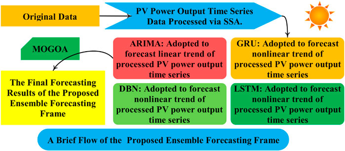
FIGURE 1. Flowchart of the proposed ensemble forecasting system (including data preprocessing, sub-model forecasting, and ensemble forecasting based on MOGOA).

2.3.1 Operating Mechanism 1: Data Preprocessing

SSA is adopted to conduct the real-time treatment of the initial PV power series, so that the dominating feature of the PV power sequence will be mastered, and effective forecasting will be conducted subsequently.

2.3.2 Operating Mechanism 2: Prediction of Hybrid Predictors

Based on the linear and nonlinear characteristics of the PV power sequence, ARIMA and DLMs were selected to build the PEFF. By combining SSA and these models, hybrid models were employed as sub-models to predict PV power. The PV power output values corresponding to the validation set were forecasted based on the rolling forecasting mechanism. Based on real data, hybrid models perform single-step and multi-step predictions. The linear model (SSA–ARIMA) in sub-models can predict the linear trend of the PV power sequence, and nonlinear models (SSA-DLMs) can predict the nonlinear trend.

The input vector of DLMs in the training set is as follows:

$input\_trai{n}_{DLMs}=\left[\begin{array}{cccc}\mathbf{yy}\left(1th\right)& \mathbf{yy}\left(2th\right)& \cdot \cdot \cdot & \mathbf{yy}\left(5th\right)\\ \mathbf{yy}\left(2th\right)& \mathbf{yy}\left(3th\right)& \cdot \cdot \cdot & \mathbf{yy}\left(6th\right)\\ ⋮& ⋮& \ddots & ⋮\\ \mathbf{yy}\left(\left(1156-k\right)th\right)& \mathbf{yy}\left(\left(1157-k\right)th\right)& \cdot \cdot \cdot & \mathbf{yy}\left(\left(1160-k\right)th\right)\end{array}\right](16)$

$output\_trai{n}_{DLMs}={\left[\begin{array}{cccc}\mathbf{y}\left(\left(5+k\right)th\right)& \mathbf{y}\left(\left(6+k\right)th\right)& \cdot \cdot \cdot & \mathbf{y}\left(1160th\right)\end{array}\right]}^{\mathrm{\top }}(17)$

The input vector of ARIMA in the training set is as follows:

$input\_trai{n}_{ARIMA}=\left[\begin{array}{cccc}\mathbf{yy}\left(1th\right)& \mathbf{yy}\left(2th\right)& \cdot \cdot \cdot & \mathbf{yy}\left(295th\right)\\ \mathbf{yy}\left(2th\right)& \mathbf{yy}\left(3th\right)& \cdot \cdot \cdot & \mathbf{yy}\left(296th\right)\\ ⋮& ⋮& \ddots & ⋮\\ \mathbf{yy}\left(\left(866-k\right)th\right)& \mathbf{yy}\left(\left(867-k\right)th\right)& \cdot \cdot \cdot & \mathbf{yy}\left(\left(1160-k\right)th\right)\end{array}\right](18)$

$output\_trai{n}_{ARIMA}={\left[\begin{array}{cccc}\mathbf{y}\left(\left(295+k\right)th\right)& \mathbf{y}\left(\left(296+k\right)th\right)& \cdot \cdot \cdot & \mathbf{y}\left(1160th\right)\end{array}\right]}^{\mathrm{\top }}(19)$

where k denotes the forecasting step, and y denotes the actual PV values, and yy denotes the processed PV values.

The input vector of DLMs in the validation set is as follows:

$input\_validatio{n}_{DLMs}=\left[\begin{array}{cccc}\mathbf{yy}\left(1157th\right)& \mathbf{yy}\left(1158th\right)& \cdot \cdot \cdot & \mathbf{yy}\left(1161th\right)\\ \mathbf{yy}\left(1158th\right)& \mathbf{yy}\left(1159th\right)& \cdot \cdot \cdot & \mathbf{yy}\left(1162th\right)\\ ⋮& ⋮& \ddots & ⋮\\ \mathbf{yy}\left(\left(1388-k\right)th\right)& \mathbf{yy}\left(\left(1389-k\right)th\right)& \cdot \cdot \cdot & \mathbf{yy}\left(\left(1392-k\right)th\right)\end{array}\right](20)$

$output\_validatio{n}_{DLMs}={\left[\begin{array}{cccc}\mathbf{y}\left(1161th\right)& \mathbf{y}\left(1162th\right)& \cdot \cdot \cdot & \mathbf{y}\left(1392th\right)\end{array}\right]}^{\mathrm{\top }}(21)$

The input vector of ARIMA in the validation set is as follows:

$input\_validatio{n}_{ARIMA}=\left[\begin{array}{cccc}\mathbf{yy}\left(\left(867-k\right)th\right)& \mathbf{yy}\left(\left(868-k\right)th\right)& \cdot \cdot \cdot & \mathbf{yy}\left(\left(1161-k\right)th\right)\\ \mathbf{yy}\left(\left(868-k\right)th\right)& \mathbf{yy}\left(\left(869-k\right)th\right)& \cdot \cdot \cdot & \mathbf{yy}\left(\left(1162-k\right)th\right)\\ ⋮& ⋮& \ddots & ⋮\\ \mathbf{yy}\left(\left(1098-k\right)th\right)& \mathbf{yy}\left(\left(1099-k\right)th\right)& \cdot \cdot \cdot & \mathbf{yy}\left(\left(1392-k\right)th\right)\end{array}\right](22)$

$output\_validatio{n}_{ARIMA}={\left[\begin{array}{cccc}\mathbf{y}\left(1161th\right)& \mathbf{y}\left(1162th\right)& \cdot \cdot \cdot & \mathbf{y}\left(1392th\right)\end{array}\right]}^{\mathrm{\top }}(23)$

where k denotes the forecasting step, and y denotes the actual PV values, and yy denotes the processed PV values.

The input vector of DLMs in the testing set is as follows:

$input\_tes{t}_{DLMs}=\left[\begin{array}{cccc}\mathbf{yy}\left(1389th\right)& \mathbf{yy}\left(1390th\right)& \cdot \cdot \cdot & \mathbf{yy}\left(1393th\right)\\ \mathbf{yy}\left(1390th\right)& \mathbf{yy}\left(1391th\right)& \cdot \cdot \cdot & \mathbf{yy}\left(1394th\right)\\ ⋮& ⋮& \ddots & ⋮\\ \mathbf{yy}\left(\left(1435-k\right)th\right)& \mathbf{yy}\left(\left(1436-k\right)th\right)& \cdot \cdot \cdot & \mathbf{yy}\left(\left(1450-k\right)th\right)\end{array}\right](24)$

$output\_tes{t}_{DLMs}={\left[\begin{array}{cccc}\mathbf{y}\left(1393th\right)& \mathbf{y}\left(1394th\right)& \cdot \cdot \cdot & \mathbf{y}\left(1450th\right)\end{array}\right]}^{\mathrm{\top }}(25)$

The input vector of ARIMA in the testing set is as follows:

$input\_tes{t}_{ARIMA}=\left[\begin{array}{cccc}\mathbf{yy}\left(\left(1099-k\right)th\right)& \mathbf{yy}\left(\left(1100-k\right)th\right)& \cdot \cdot \cdot & \mathbf{yy}\left(\left(1393-k\right)th\right)\\ \mathbf{yy}\left(\left(1100-k\right)th\right)& \mathbf{yy}\left(\left(1101-k\right)th\right)& \cdot \cdot \cdot & \mathbf{yy}\left(\left(1394-k\right)th\right)\\ ⋮& ⋮& \ddots & ⋮\\ \mathbf{yy}\left(\left(1156-k\right)th\right)& \mathbf{yy}\left(\left(1157-k\right)th\right)& \cdot \cdot \cdot & \mathbf{yy}\left(\left(1450-k\right)th\right)\end{array}\right](26)$

$output\_validatio{n}_{ARIMA}={\left[\begin{array}{cccc}\mathbf{y}\left(1393th\right)& \mathbf{y}\left(1394th\right)& \cdot \cdot \cdot & \mathbf{y}\left(1450th\right)\end{array}\right]}^{\mathrm{\top }}(27)$

where k denotes the forecasting step, and y denotes the actual PV values, and yy denotes the processed PV values.

2.3.3 Operating Mechanism 3: Ensemble Forecasting

In this stage, MOGOA is applied to determine the best weight coefficient of the forecasting values of each sub-model. Based on MOGOA, prediction values matching the validation set of four prediction sub-models obtained from Process 2 are used to search for the best weight coefficient of each sub-model, and real values matching the testing set are used to test the forecasting performance of the PEFF. Finally, the final PV power prediction result is aggregated via the prediction values matching the testing set of each sub-model and the optimal weight coefficients corresponding to each sub-model. The objective functions of MOGOA are prediction accuracy and stability in PEFF, and its fitness function is provided:

$min\{\begin{array}{l}O{b}_1=mean\left(abs\left(\mathbf{y}-\widehat{\mathbf{y}}\right)/\mathbf{y}\right)\times 100\mathbf{\%}\\ O{b}_2=std\left(\mathbf{y}-\widehat{\mathbf{y}}\right)\end{array}(28)$

where y denotes the actual PV values, and $\widehat{y}$ denotes the forecasting PV values.

The fitness function can be rewritten as:

$\{\begin{array}{l}\left\{\mathit{w}\right\}=\mathit{arg}\underset{\left\{\mathrm{w}\right\}}{\mathit{min}}\{\begin{array}{l}O{b}_1=mean\left(abs\left(\mathbf{y}-\widehat{\mathbf{y}}\right)/\mathbf{y}\right)\times 100\text{\%}\\ O{b}_2=std\left(\mathbf{y}-\widehat{\mathbf{y}}\right)\end{array}\\ s.t.-2\le \mathit{w}\le 2\\ \widehat{\mathbf{y}}=sub\_{\widehat{y}}_{\mathit{ARIMA}}\times {\mathit{w}}_{ARIMA}+sub\_{\widehat{y}}_{DBN}\times {\mathit{w}}_{DBN}\\ +sub\_{\widehat{y}}_{GRU}\times {\mathit{w}}_{GRU}+sub\_{\widehat{y}}_{LSTM}\times {\mathit{w}}_{LSTM},\\ \mathit{w}=\left\{{\mathit{w}}_{ARIMA},{\mathit{w}}_{DBN},{\mathit{w}}_{GRU},{\mathit{w}}_{LSTM}\right\}\end{array}(29)$

The weights are optimized to achieve good forecasting performance in validation set by MOGOA. Ultimately, the final forecasting results are calculated as $\widehat{\mathbf{y}}\left(1393th-1450th\right)$.

2.3.4 Operating Mechanism 4: Forecasting Performance Assessment

The forecasting accuracy and stability were assessed using four indicators (see Table 2 for details) based on three experiments, and five discussions were held to further analyze the prediction effect of PEFF.

TABLE 2

TABLE 2. Four performance indicators.

3 Experimental Setup and Result Analyses

In this section, the experimental setup and forecasting result analyses based on three PV power datasets are presented to verify the forecasting ability of our PEFF.

3.1 Datasets

Initial PV power data were acquired from three datasets in Belgium with a time interval of 15 min. When the light intensity reaches a certain level, the PV power generation has sufficient output; therefore, this study considers PV power generation data from 9:00 to 16:00 every day as the verification dataset. Specifically, 1,450 data points for continuous 50 days from different time period were adopted as the reference dataset. The detailed data characteristics of the PEFF are shown in Figure 2.

FIGURE 2

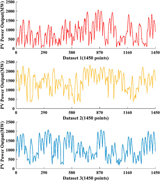
FIGURE 2. Original PV power output time series in these studied datasets.

There is no official or specific procedure to select the optimal training-to-test ratio. In actual application, with the improvement of training-to-test, the forecasting accuracy can be obviously improved, while too many training data may result in overfitting issue. In this paper, based on previous experiences and researches, the ratio of training, validation, and test set is set to 20:4:1. Specifically, the 1st–1160th values were selected as the training set, the 1161st-1392nd values were considered as the validation set, and the 1393th-1450th values were selected as the testing set. The relevant data characteristics are listed in Table 3.

TABLE 3

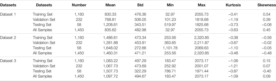
TABLE 3. Relevant data characteristics of three datasets.

3.2 Assessment Indicators of Forecasting Performance

There must be a scientific evaluation system to determine whether the prediction performance is satisfactory. In this section, four indicators, including the mean absolute error (MAE), mean absolute percent error (MAPE), root mean square error (RMSE), and standard deviation of error (SDE), are introduced to verify the forecasting effort of our PEFF. The concepts and equations of the four indicators are listed in Table 2.

3.3 Experimental Setup

Based on the PV power dataset, three experiments were designed to compare the PEFF and reference models. In these experiments, Experiment I contrasted the prediction ability of the PEFF and hybrid models. Experiment II compared the PEFF with the EFs, employing different data pretreatment strategies and MOOAs in terms of forecasting effect. Experiment III compared the prediction capacity of the PEFF and classical models. The prediction ability of 1-step to 3-step prediction is testified via four indicators, and experimental result analyses are described.

Experiment I was conducted to verify the advantages of PEFF compared with hybrid models. The parameter setting of the SSA is the same as that of the PEFF, and the rolling number of the models was set to 5.

Experiment II was conducted to prove that the ensemble learning strategy of PEFF surpasses the EFs structured via other data pretreatment techniques (complete ensemble empirical mode decomposition (CEEMD)) and MOOAs (multi-objective dragonfly algorithm (MODA) and multi-objective grey wolf optimizer (MOGWO)). For each EF, the ensemble learning strategy changes, and the input and output settings remain unchanged.

Experiment III was employed to reveal the forecasting superiority of the PEFF with classical models (backpropagation (BP) neural network, extreme learning machine (ELM), Elman neural network (ENN), echo state network (ESN), least squares support vector machine (LSSVM) and radical basis function (RBF)).

3.4 Experiment I: Comparison With Hybrid Predictors

The experimental results are listed in Table 4. For Dataset 1, PEFF has an unrivaled characteristic in one-step and multi-step predictions. In particular, the MAPE value is 1.7722% in one-step, 2.5428% in two-step, and 4.3568% in three-step predictions, which are minimum compared with the involved models. For Dataset 2, the lowest MAE, MAPE, RMSE, and SDE were obtained from the PEFF in one step, with values of 13.5285, 0.9495%, 21.3817, and 21.5428, respectively. In multi-step prediction, the most satisfactory results are achieved by the PEFF, confirming the forecasting effect of our PEFF. For Dataset 3, the forecasting accuracy and stability of PEFF signally precede that of the reference models. This implies that although hybrid models can improve the prediction precision weakly, the PEFF is better.

TABLE 4

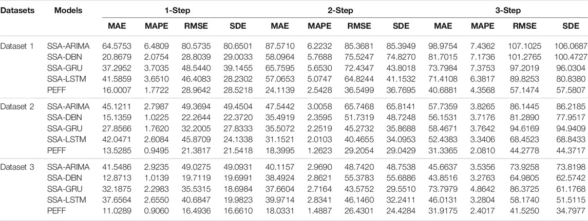
TABLE 4. Comparison of the prediction performance of the PEFF and hybrid models.

Remark. The PEFF obtains a more satisfactory prediction ability with the smallest error indicator values among all of the involved models, proving the short-term prediction availability of the proposed PEFF in PV power output.

3.5 Experiment II: Comparison With EFs Adopting Diverse Ensemble Strategies

Experiment II compares the EFs with different data pretreatment techniques (CEEMD) and MOOAs (MODA and MOGWO). The forecasting results are listed in Table 5. For Dataset 1, the PEFF is precise and stabilized in PV power prediction, which can be concluded based on the MAPE values (1.7722, 2.5428, and 4.3568%) in each forecasting step. For Dataset 2, the four assessment indicator values in each forecasting step obtained from PEFF are the most satisfactory. The MAPE in one-step forecasting obtained from the PEFF is 0.9495%, which is 0.2132% higher than that of SSA-MOGWO-EF, which is second in the prediction effect. As for Dataset 3, regardless of the prediction step, the PEFF obtains the optimal forecasting result proved by obviously lower error indicator values. For instance, in three steps, the PEFF provides the lowest MAE, MAPE, RMSE, and SDE of 31.9175, 2.4017%, 41.5250, and 34.7977, respectively, while the highest MAPE was obtained from CEEMD-MOGOA-EF at 4.8862%.

TABLE 5

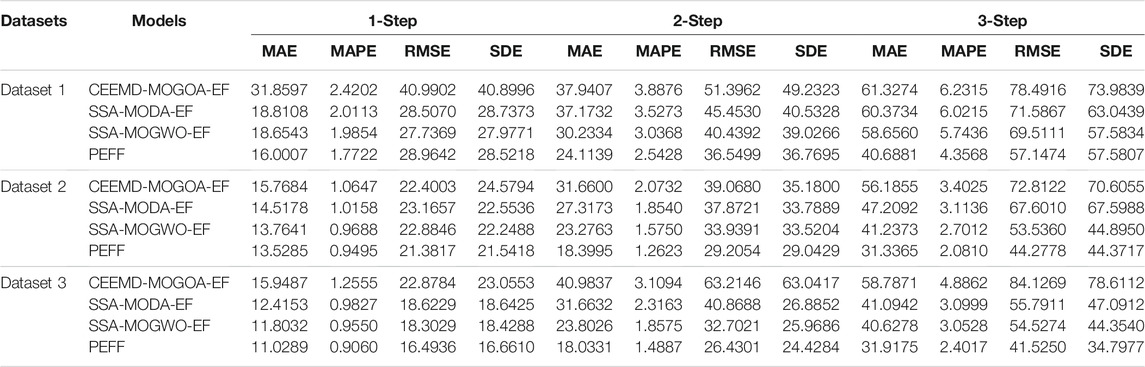
TABLE 5. Comparison of the forecasting performance of the PEFF and EFs employing other ensemble strategies.

Remark. The assessment indicator values in Experiment II show that the PEFF precedes the EFs based on other ensemble strategies in terms of forecasting precision and stability, regardless of the prediction step and dataset.

3.6 Experiment III: Comparison With Classic Models

The experimental results reveal the forecasting ability of the PV power sequence by comparing the PEFF with classic models (BP, ELM, ENN, ESN, LSSVM, and RBF). The prediction results are listed in Table 6. For Dataset 1, with regard to the one-step prediction, PEFF exhibits the optimal forecasting performance. With regard to two- and three-step forecasting processes, the assessment indicators of the PEFF are minimally compared with the classical models, which indicate that the PEFF is more valid in PV power prediction. For Dataset 2, classical models achieved unsatisfactory prediction effects with higher values of MAE, MAPE, RMSE, and SDE. Specifically, in 2-step forecasting, the MAPE values of BP, ELM, ENN, ESN, LSSVM, and RBF are 7.6081, 7.5464, 7.8467, 9.1621, 7.9522, and 7.1286%, respectively, and the MAPE values of PEFF were 1.2623, 6.3458, 6.2841, 6.5844, 7.8999, 6.6899, and 5.8664%. As for Dataset 3, the PEFF precedes other involved models with average values of the evaluation criteria of 20.3265, 1.5988%, 28.1495, and 25.2957, respectively, in three steps.

TABLE 6

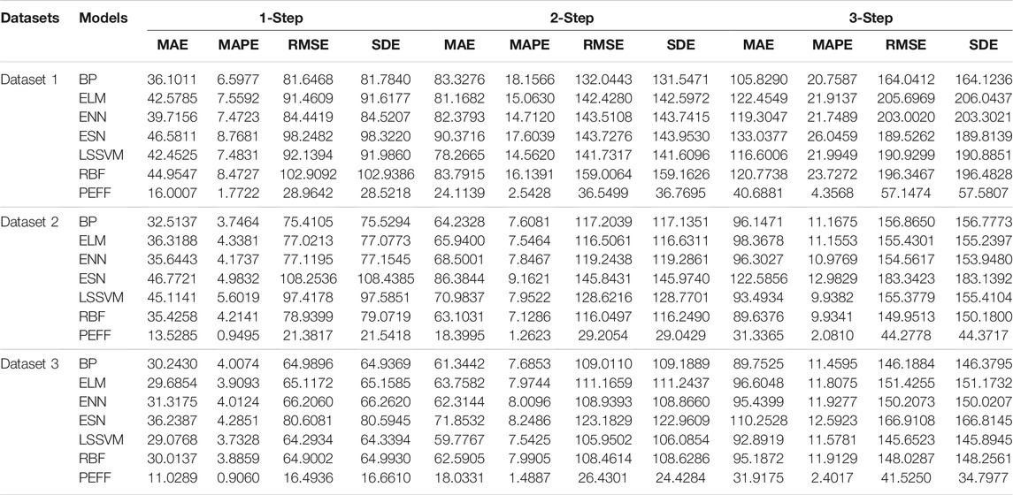
TABLE 6. Comparison of the prediction performance of the PEFF and reference models.

Remark. Based on the results of this experiment, we can conclude that the PEFF has a stronger effect than the classical models in short-term PV power prediction.

4 Discussion

In this section, the PEFF is discussed in detail, including the significance, sensitivity analysis, operational efficiency, practical applications, defects, and future directions of the PEFF.

4.1 Forecasting Significance of the PEFF

To investigate whether there is a prominent difference in the prediction ability between the PEFF and reference models, the Diebold–Mariano (DM) test (Jiang et al., 2021) was conducted. The concrete theory of this test can be found in (Zhang et al., 2021).

As for our study, Table 7 lists the DM values from 1-step to 3-step prediction based on the three datasets. First, the PEFF is different from classical models (BP, ELM, ENN, ESN, LSSVM, and RBF) at a significance level of 99%. Moreover, although the DM values computed based on the difference between the PEFF and hybrid models are lower than that computed based on the difference between the PEFF and each classical model, the PEFF has a distinguishing prediction capacity compared with each hybrid model at a significance level of 95%. Then, when comparing the PEFF with the EFs adopting disparate ensemble strategies, the DM statistical magnitude pertaining to one-step to three-step prediction based on each dataset exceeds the critical value at a significance level of 95%, which illustrates that there is a 95% possibility that we will not reject H₁.

TABLE 7

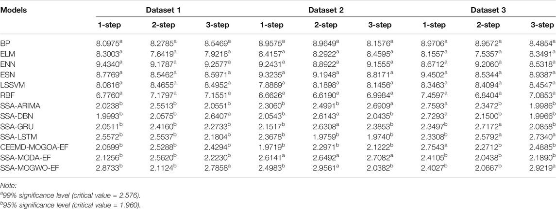
TABLE 7. DM results of the models included in this study.

Based on the DM statistical magnitude, the forecasting results of PEFF are significantly different from those of classical models (BP, ELM, ENN, ESN, LSSVM, and RBF), hybrid models (SSA-ARIMA, SSA-DBN, SSA-GRU, and SSA-LSTM), and EFs using diverse ensemble strategies (CEEMD-MOGOA-EF, SSA-MODA-EF, and SSA-MOGWO-EF). Thus, it is valuable to exploit PEFF and employ it in practical PV power forecasting.

4.2 Sensitivity Analysis of the PEFF

To explore the prediction ability of the PEFF when a certain parameter changes, sensitivity analysis was performed to measure the output result sensitivity of PEFF based on the parameter settings of SSA and MOGOA. The standard deviation (STD) of error indicators, as shown in Table 8, was adopted to assess the level at which the parameter setting impacted the properties of PEFF (Liu et al., 2021). The results of the sensitivity analysis are listed in Table 9, where the window length and principal component decomposition number (PCDN) belong to SSA and the population size, iteration number, and archive size belong to MOGOA.

TABLE 8

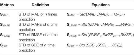
TABLE 8. Four designed indicators of sensitivity analysis.

TABLE 9

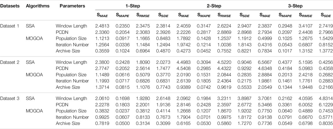
TABLE 9. STD values of the results acquired by changing parameters.

Sensitivity analyses were conducted by changing one parameter, and the remaining parameters remained unchanged. It must be known that each parameter value is assigned as 40, 45, 50, 55, and 60 in terms of window length, and 10, 15, 20, 25, and 30 in terms of PCDN, respectively. Meanwhile, the parameter is set as 10, 30, 50, 70, and 90 in terms of population size; 300, 400, 500, 600, and 700 in terms of iteration number; and 100, 150, 200, 250, and 300 in terms of archive size.

(1) As the parameters of SSA change, the S_MAE, S_MAPE, S_RMSE, and S_SDE values of the two parameters become higher. For instance, in the three-step prediction based on Dataset 1, the S_MAPE value is 0.2948 for window length and 0.2097 for PCDN, which are lower than the S_SDE values but still higher than the S_MAPE values of MOGOA parameters. The above results indicate that the SSA significantly impacts the forecasting performance of the PEFF.

(2) When the parameter in MOGOA is altered, compared with the sensitivity analysis results obtained from SSA, the measured indicators of MOGOA are lower than those of SSA, indicating that the fluctuation of forecasting performance generated by parameter alteration in MOGOA is slight.

4.3 Operational Efficiency of the PEFF

To further explore the operational efficiency of PEFF, the run time of each model based on three datasets, regardless of the forecasting step, is listed in Table 10. In particular, the mean value of the operational time of the PEFF is 164.5339 s, which is shorter than the EFs based on different ensemble strategies. The computing time of PEFF is shorter than that of SSA-MODA-EF, which confirms the superiority of the MOGOA adopted in PEFF. Moreover, in contrast to hybrid and classical models, the average operational time of PEFF is longer, which is reasonable owing to its excellent prediction ability. The operational efficiency of the PEFF can be improved by adopting a high-powered computer.

TABLE 10

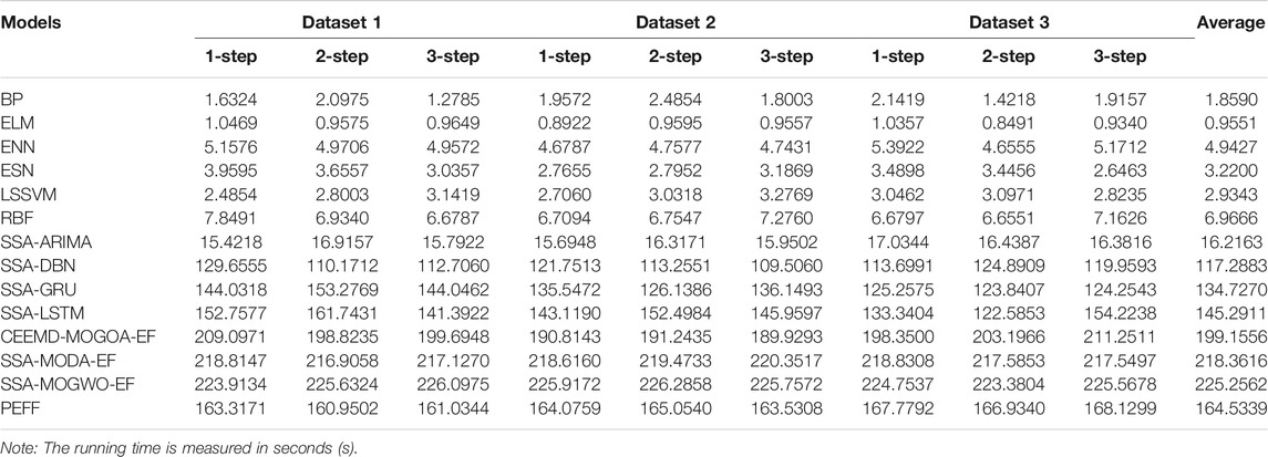
TABLE 10. Run time of each model.

4.4 Practical Applications of the PEFF

In practical scenarios, real-time missions considering PV power generation planning and grid security safeguards require effective forecasting. In particular, precise and stable PV power prediction can solve the challenge caused by the irregular undulations of PV power, which is the key point for the businesslike running of PV power generation systems and can improve the stability and efficiency of the energy market and energy industry. Accurate and stable PV power forecasting can also effectively boost the PV penetration degree, reduce the use of fossil fuels, and enhance economic and environmental benefits, which is conductive to the sustainable development of the society.

Moreover, the forecasting results of the PV power output support decision-makers in maintaining the power system stability, installing large PV power stations, and monitoring the security of power systems. When the predicted PV power output result is inconsistent with the real data, energy producers can assess efficiency degradation caused by motor aging or motor faults and deal with it in time to reduce economic loss. In other words, accurate PV output forecasting provides valuable assistance for monitoring the running status of equipment, which saves maintenance costs and reduces the risk of power grid breakdown.

Furthermore, accurate forecasting is essential for grid operators to help them determine balancing power that can satisfy unnecessary demand for fossil fuels. By referring to PV power forecasting results, decision makers can determine reasonable power supply volumes of PV power and fossil fuel power plants so as to satisfy the country’s power demand. Meanwhile, accurate PV power forecasting is conductive to setting reasonable rotating reserve capacity so as to enhance energy economy and reduce the risk of PV abandonment.

4.5 Defects and Future Directions

The main limitation of PEFF is that the applied area is limited to power systems containing PV power stations, instead of finance, such as future price predictions.

After PV power prediction, adaptable improvements for future are as follows:

(1) Finding more effective data preprocessing methods to process PV power data and process the irregular characteristics of the initial PV power data more effectively.

(2) Enhancing sub-models to provide satisfactory forecasting results for the subsequent forecasting of EF.

(3) The operation efficiency of the proposed PEFF should be improved by GPU acceleration.

(4) More underlying external factors, such as weather and solar irradiation, must be taken into consideration to obtain better forecasting results for longer forecasting horizons.

5 Conclusion

We developed an ensemble forecasting frame that capitalizes the data preprocessing technique and optimization algorithm to forecast PV power. The proposed system has been proved to be effective and efficient to improve the prediction accuracy and stability of short-term PV power. Specifically, a data preprocessing technique is employed to disintegrate the original PV power sequence and integrate a processed sequence to decrease prediction errors created by the irregular undulations of the PV power series. ARIMA and three DLMs were adopted as sub-models to forecast PV power sequences. Further, MOGOA was adopted to compute the weight of each sub-model of the PEFF and obtain the final prediction result. Simulation results prove that the proposed system (SSA–MOGOA–EF) surpasses the comparative models. Specifically, in Experiment I, the lowest average MAPE based on each dataset was obtained from PEFF with values of 2.89, 1.43, and 1.60%, which were reduced by 3.82, 1.78, and 1.54%, respectively, compared with the maximum values obtained from SSA–ARIMA. This revels that the proposed ensemble forecasting scheme is obviously superior to the comparative hybrid models in terms of accuracy and stability. The ensemble strategy can successfully improve short-term PV power forecasting performance. In Experiments II, the MAPE values of PEFF based on all datasets are the most satisfactory, which implies that the PEFF based on SSA and MOGOA technologies exceeds the comparative ensemble models based on other data preprocessing technologies and optimization algorithms. Thus, it is a wise choice to use SSA–MOGOA–EF for PV power forecasting. Similarly, in Experiment III, the improvement of the proposed forecasting system over the classical individual models is more significant, further testifies the effectiveness of the proposed ensemble system. Five discussions are further conducted to testify the performance of the proposed frame. Based on the discussions, we testify that there is an observable difference between the prediction results of the PEFF and the benchmark models, and the proposed forecasting frame is less sensitive to the parameter change of MOGOA than that of SSA. Furthermore, the proposed forecasting frame incurs a lower cost compared with EFs adopting other ensemble strategies. Thus, we can conclude that the PEFF successfully improves the forecasting accuracy and stability of PV power and can achieve more efficient and time-saving forecasting results, which can provide useful support for smart grid planning.

Data Availability Statement

The original contributions presented in the study are included in the article/Supplementary Material, further inquiries can be directed to the corresponding author.

Author Contributions

Software, YL; Supervision, LL; Writing—original draft, SZ; Writing—review and editing, YL.

Conflict of Interest

The authors declare that the research was conducted in the absence of any commercial or financial relationships that could be construed as a potential conflict of interest.

Publisher’s Note

All claims expressed in this article are solely those of the authors and do not necessarily represent those of their affiliated organizations, or those of the publisher, the editors and the reviewers. Any product that may be evaluated in this article, or claim that may be made by its manufacturer, is not guaranteed or endorsed by the publisher.

Footnotes

¹https://news.solarbe.com/202004/29/324368.html.

References

Abdel-Nasser, M., and Mahmoud, K. (2019). Accurate Photovoltaic Power Forecasting Models Using Deep LSTM-RNN. Neural Comput. Applic 31, 2727–2740. doi:10.1007/s00521-017-3225-z

CrossRef Full Text | Google Scholar

Agga, A., Abbou, A., Labbadi, M., and El Houm, Y. (2021). Short-Term Self Consumption PV Plant Power Production Forecasts Based on Hybrid CNN-LSTM, ConvLSTM Models. Renew. Energ. 177, 101–112. doi:10.1016/j.renene.2021.05.095

CrossRef Full Text | Google Scholar

Aygül, K., Cikan, M., Demirdelen, T., and Tumay, M. (2019). Butterfly Optimization Algorithm Based Maximum Power point Tracking of Photovoltaic Systems under Partial Shading Condition. Energy Sourc. A: Recovery, Utilization, Environ. Effects, 1–19. doi:10.1080/15567036.2019.1677818

CrossRef Full Text | Google Scholar

Bates, J. M., and Granger, C. W. J. (1969). Combination of Forecasts. Oper. Res. Q.

Google Scholar

Das, N., Wongsodihardjo, H., and Islam, S. (2015). Modeling of Multi-junction Photovoltaic Cell Using MATLAB/Simulink to Improve the Conversion Efficiency. Renew. Energ. 74, 917–924. doi:10.1016/j.renene.2014.09.017

CrossRef Full Text | Google Scholar

David, M., Ramahatana, F., Trombe, P. J., and Lauret, P. (2016). Probabilistic Forecasting of the Solar Irradiance with Recursive ARMA and GARCH Models. Solar Energy 133, 55–72. doi:10.1016/j.solener.2016.03.064

CrossRef Full Text | Google Scholar

de Carvalho, M., and Rua, A. (2017). Real-time Nowcasting the US Output gap: Singular Spectrum Analysis at Work. Int. J. Forecast. 33, 185–198. doi:10.1016/j.ijforecast.2015.09.004

CrossRef Full Text | Google Scholar

Devaraj, J., Madurai Elavarasan, R., Shafiullah, G., Jamal, T., and Khan, I. (2021). A Holistic Review on Energy Forecasting Using Big Data and Deep Learning Models. Int. J. Energ. Res. 45, 13489–13530. doi:10.1002/er.6679

CrossRef Full Text | Google Scholar

Dong, J., Olama, M. M., Kuruganti, T., Melin, A. M., Djouadi, S. M., Zhang, Y., et al. (2020). Novel Stochastic Methods to Predict Short-Term Solar Radiation and Photovoltaic Power. Renew. Energ. 145, 333–346. doi:10.1016/j.renene.2019.05.073

CrossRef Full Text | Google Scholar

Elavarasan, R. M., Leoponraj, S., Vishnupriyan, J., Dheeraj, A., and Gangaram Sundar, G. (2021). Multi-Criteria Decision Analysis for User Satisfaction-Induced Demand-Side Load Management for an Institutional Building. Renew. Energ. 170, 1396–1426. doi:10.1016/j.renene.2021.01.134

CrossRef Full Text | Google Scholar

Elsinga, B., and van Sark, W. G. J. H. M. (2017). Short-term Peer-To-Peer Solar Forecasting in a Network of Photovoltaic Systems. Appl. Energ. 206, 1464–1483. doi:10.1016/j.apenergy.2017.09.115

CrossRef Full Text | Google Scholar

Eseye, A. T., Zhang, J., and Zheng, D. (2018). Short-term Photovoltaic Solar Power Forecasting Using a Hybrid Wavelet-PSO-SVM Model Based on SCADA and Meteorological Information. Renew. Energ. 118, 357–367. doi:10.1016/j.renene.2017.11.011

CrossRef Full Text | Google Scholar

Feng, C., Cui, M., Hodge, B.-M., and Zhang, J. (2017). A Data-Driven Multi-Model Methodology with Deep Feature Selection for Short-Term Wind Forecasting. Appl. Energ. 190, 1245–1257. doi:10.1016/j.apenergy.2017.01.043

CrossRef Full Text | Google Scholar

Hao, Y., and Tian, C. (2019). The Study and Application of a Novel Hybrid System for Air Quality Early-Warning. Appl. Soft Comput. 74, 729–746. doi:10.1016/j.asoc.2018.09.005

CrossRef Full Text | Google Scholar

Hassani, H., and Ghodsi, Z. (2015). A Glance at the Applications of Singular Spectrum Analysis in Gene Expression Data. Biomol. Detect. Quantification 4, 17–21. doi:10.1016/j.bdq.2015.04.001

PubMed Abstract | CrossRef Full Text | Google Scholar

Irfan, M., Elavarasan, R. M., Hao, Y., Feng, M., and Sailan, D. (2021). An Assessment of Consumers' Willingness to Utilize Solar Energy in China: End-Users' Perspective. J. Clean. Prod. 292, 126008. doi:10.1016/j.jclepro.2021.126008

CrossRef Full Text | Google Scholar

Islam, S. (2017). “Challenges and Opportunities in Grid Connected Commercial Scale PV and Wind Farms,” in Proc. 9th Int. Conf. Electr. Comput. Eng. ICECE 2016, 1–7. doi:10.1109/ICECE.2016.7853843

CrossRef Full Text | Google Scholar

Iversen, E. B., Morales, J. M., Møller, J. K., and Madsen, H. (2016). Short-term Probabilistic Forecasting of Wind Speed Using Stochastic Differential Equations. Int. J. Forecast. 32, 981–990. doi:10.1016/j.ijforecast.2015.03.001

CrossRef Full Text | Google Scholar

Jiang, P., Liu, Z., Niu, X., and Zhang, L. (2021). A Combined Forecasting System Based on Statistical Method, Artificial Neural Networks, and Deep Learning Methods for Short-Term Wind Speed Forecasting. Energy 217, 119361-11936. doi:10.1016/j.energy.2020.119361

CrossRef Full Text | Google Scholar

Jiang, P., and Liu, Z. (2019). Variable Weights Combined Model Based on Multi-Objective Optimization for Short-Term Wind Speed Forecasting. Appl. Soft Comput. 82, 105587. doi:10.1016/j.asoc.2019.105587

CrossRef Full Text | Google Scholar

Jiang, P., Liu, Z., Wang, J., and Zhang, L. (2021). Decomposition-selection-ensemble Forecasting System for Energy Futures price Forecasting Based on Multi-Objective Version of Chaos Game Optimization Algorithm. Resour. Pol. 73, 102234. doi:10.1016/j.resourpol.2021.102234

CrossRef Full Text | Google Scholar

Korkmaz, D. (2021). SolarNet: A Hybrid Reliable Model Based on Convolutional Neural Network and Variational Mode Decomposition for Hourly Photovoltaic Power Forecasting. Appl. Energ. 300, 117410. doi:10.1016/j.apenergy.2021.117410

CrossRef Full Text | Google Scholar

Krishnannair, S., Aldrich, C., and Jemwa, G. T. (2016). Detecting Faults in Process Systems with Singular Spectrum Analysis. Chem. Eng. Res. Des. 113, 151–168. doi:10.1016/j.cherd.2016.07.014

CrossRef Full Text | Google Scholar

Kushwaha, V., and Pindoriya, N. M. (2019). A SARIMA-RVFL Hybrid Model Assisted by Wavelet Decomposition for Very Short-Term Solar PV Power Generation Forecast. Renew. Energ. 140, 124–139. doi:10.1016/j.renene.2019.03.020

CrossRef Full Text | Google Scholar

Li, C. (2020). Designing a Short-Term Load Forecasting Model in the Urban Smart Grid System. Appl. Energ. 266, 114850. doi:10.1016/j.apenergy.2020.114850

CrossRef Full Text | Google Scholar

Li, P., Zhou, K., Lu, X., and Yang, S. (2020). A Hybrid Deep Learning Model for Short-Term PV Power Forecasting. Appl. Energ. 259, 114216. doi:10.1016/j.apenergy.2019.114216

CrossRef Full Text | Google Scholar

Liu, L., Zhao, Y., Wang, Y., Sun, Q., and Wennersten, R. (2019). “A Weight-Varying Ensemble Method for Short-Term Forecasting PV Power Output,” in Energy Procedia, 158, 661–668. doi:10.1016/j.egypro.2019.01.180Energ. Proced.

CrossRef Full Text | Google Scholar

Liu, Z., Jiang, P., Wang, J., and Zhang, L. (2021). Ensemble Forecasting System for Short-Term Wind Speed Forecasting Based on Optimal Sub-model Selection and Multi-Objective Version of Mayfly Optimization Algorithm. Expert Syst. Appl. 177, 114974-11497. doi:10.1016/j.eswa.2021.114974

CrossRef Full Text | Google Scholar

Liu, Z., Jiang, P., Wang, J., and Zhang, L. (2022). Ensemble System for Short Term Carbon Dioxide Emissions Forecasting Based on Multi-Objective tangent Search Algorithm. J. Environ. Manage. 302, 113951. doi:10.1016/j.jenvman.2021.113951

CrossRef Full Text | Google Scholar

Liu, Z., Jiang, P., Zhang, L., and Niu, X. (2020). A Combined Forecasting Model for Time Series: Application to Short-Term Wind Speed Forecasting. Appl. Energ. 259, 114137. doi:10.1016/j.apenergy.2019.114137

CrossRef Full Text | Google Scholar

Luo, X., Zhang, D., and Zhu, X. (2021). Deep Learning Based Forecasting of Photovoltaic Power Generation by Incorporating Domain Knowledge. Energy 225, 120240. doi:10.1016/j.energy.2021.120240

CrossRef Full Text | Google Scholar

Mellit, A., Pavan, A. M., and Lughi, V. (2021). Deep Learning Neural Networks for Short-Term Photovoltaic Power Forecasting. Renew. Energ. 172, 276–288. doi:10.1016/j.renene.2021.02.166

CrossRef Full Text | Google Scholar

Mirjalili, S. Z., Mirjalili, S., Saremi, S., Faris, H., and Aljarah, I. (2018). Grasshopper Optimization Algorithm for Multi-Objective Optimization Problems. Appl. Intell. 48, 805–820. doi:10.1007/s10489-017-1019-8

CrossRef Full Text | Google Scholar

Nie, Y., Jiang, P., and Zhang, H. (2020). A Novel Hybrid Model Based on Combined Preprocessing Method and Advanced Optimization Algorithm for Power Load Forecasting. Appl. Soft Comput. 97, 106809. doi:10.1016/j.asoc.2020.106809

CrossRef Full Text | Google Scholar

Niu, D., Wang, K., Sun, L., Wu, J., and Xu, X. (2020). Short-term Photovoltaic Power Generation Forecasting Based on Random forest Feature Selection and CEEMD: A Case Study. Appl. Soft Comput. 93, 106389. doi:10.1016/j.asoc.2020.106389

CrossRef Full Text | Google Scholar

Niu, X., and Wang, J. (2019). A Combined Model Based on Data Preprocessing Strategy and Multi-Objective Optimization Algorithm for Short-Term Wind Speed Forecasting. Appl. Energ. 241, 519–539. doi:10.1016/j.apenergy.2019.03.097

CrossRef Full Text | Google Scholar

Opitz, D., and Maclin, R. (1999). Popular Ensemble Methods: An Empirical Study. jair 11, 169–198. doi:10.1613/jair.614

CrossRef Full Text | Google Scholar

Pedro, H. T. C., and Coimbra, C. F. M. (2012). Assessment of Forecasting Techniques for Solar Power Production with No Exogenous Inputs. Solar Energy 86, 2017–2028. doi:10.1016/j.solener.2012.04.004

CrossRef Full Text | Google Scholar

Qu, J., Qian, Z., and Pei, Y. (2021a). Day-ahead Hourly Photovoltaic Power Forecasting Using Attention-Based CNN-LSTM Neural Network Embedded with Multiple Relevant and Target Variables Prediction Pattern. Energy 232, 120996-12099. doi:10.1016/j.energy.2021.120996

CrossRef Full Text | Google Scholar

Qu, Y., Xu, J., Sun, Y., and Liu, D. (2021b). A Temporal Distributed Hybrid Deep Learning Model for Day-Ahead Distributed PV Power Forecasting. Appl. Energ. 304, 117704. doi:10.1016/j.apenergy.2021.117704

CrossRef Full Text | Google Scholar

Sharma, N., Mangla, M., Yadav, S., Goyal, N., Singh, A., Verma, S., et al. (2021). A Sequential Ensemble Model for Photovoltaic Power Forecasting. Comput. Electr. Eng. 96, 107484. doi:10.1016/j.compeleceng.2021.107484

CrossRef Full Text | Google Scholar

Shelat, N., Das, N., Khan, M. M. K., and Islam, S. (2019). “Nano-structured Photovoltaic Cell Design for High Conversion Efficiency by Optimizing Various Parameters,” in 2019 29th Australas. Univ. Power Eng. Conf. AUPEC 2019, 26–29. doi:10.1109/AUPEC48547.2019.211859

CrossRef Full Text | Google Scholar

Shezan, S. K. A., Das, N., and Mahmudul, H. (2017). Techno-economic Analysis of a Smart-Grid Hybrid Renewable Energy System for Brisbane of Australia. Energ. Proced. 110, 340–345. doi:10.1016/j.egypro.2017.03.150

CrossRef Full Text | Google Scholar

S., J., and M., R. (2018). “Reconfigurable Solar Converter with Inverter, Chopper and Rectifier Operation for Residential PV Applications,” in Proc. 2018 IEEE Int. Conf. Power Electron. Drives Energy Syst. PEDES 2018, 1–4. doi:10.1109/PEDES.2018.8707571

CrossRef Full Text | Google Scholar

Soubdhan, T., Ndong, J., Ould-Baba, H., and Do, M.-T. (2016). A Robust Forecasting Framework Based on the Kalman Filtering Approach with a Twofold Parameter Tuning Procedure: Application to Solar and Photovoltaic Prediction. Solar Energy 131, 246–259. doi:10.1016/j.solener.2016.02.036

CrossRef Full Text | Google Scholar

Takilalte, A., Harrouni, S., and Mora, J. (2019). Forecasting Global Solar Irradiance for Various Resolutions Using Time Series Models - Case Study: Algeria. Energ. Sourc. Part A: Recovery, Utilization, Environ. Effects 0, 1–20. doi:10.1080/15567036.2019.1649756

CrossRef Full Text | Google Scholar

Tan, B., Raga, S. R., Rietwyk, K. J., Lu, J., Fürer, S. O., Griffith, J. C., et al. (2021). The Impact of spiro-OMeTAD Photodoping on the Reversible Light-Induced Transients of Perovskite Solar Cells. Nano Energy 82, 105658. doi:10.1016/j.nanoen.2020.105658

CrossRef Full Text | Google Scholar

Tanaka, K., Uchida, K., Ogimi, K., Goya, T., Yona, A., Senjyu, T., et al. (2011). Optimal Operation by Controllable Loads Based on Smart Grid Topology Considering Insolation Forecasted Error. IEEE Trans. Smart Grid 2, 438–444. doi:10.1109/TSG.2011.2158563

CrossRef Full Text | Google Scholar

Tian, C., and Hao, Y. (2018). A Novel Nonlinear Combined Forecasting System for Short-Term Load Forecasting. Energies 11, 712. doi:10.3390/en11040712

CrossRef Full Text | Google Scholar

Unnikrishnan, P., and Jothiprakash, V. (2018). Daily Rainfall Forecasting for One Year in a Single Run Using Singular Spectrum Analysis. J. Hydrol. 561, 609–621. doi:10.1016/j.jhydrol.2018.04.032

CrossRef Full Text | Google Scholar

Wang, J., Li, Q., and Zeng, B. (2021). Multi-layer Cooperative Combined Forecasting System for Short-Term Wind Speed Forecasting. Sustainable Energ. Tech. Assessments 43, 100946. doi:10.1016/j.seta.2020.100946

CrossRef Full Text | Google Scholar

Xiao, L., Wang, J., Dong, Y., and Wu, J. (2015). Combined Forecasting Models for Wind Energy Forecasting: A Case Study in China. Renew. Sustain. Energ. Rev. 44, 271–288. doi:10.1016/j.rser.2014.12.012

CrossRef Full Text | Google Scholar

Yacef, R., Mellit, A., Belaid, S., and Şen, Z. (2014). New Combined Models for Estimating Daily Global Solar Radiation from Measured Air Temperature in Semi-arid Climates: Application in Ghardaïa, Algeria. Energ. Convers. Manage. 79, 606–615. doi:10.1016/j.enconman.2013.12.057

CrossRef Full Text | Google Scholar

Yagli, G. M., Yang, D., and Srinivasan, D. (2019). Automatic Hourly Solar Forecasting Using Machine Learning Models. Renew. Sustain. Energ. Rev. 105, 487–498. doi:10.1016/j.rser.2019.02.006

CrossRef Full Text | Google Scholar

Yang, D., and Dong, Z. (2018). Operational Photovoltaics Power Forecasting Using Seasonal Time Series Ensemble. Solar Energy 166, 529–541. doi:10.1016/j.solener.2018.02.011

CrossRef Full Text | Google Scholar

Yildiz, C., and Acikgoz, H. (2021). A Kernel Extreme Learning Machine-Based Neural Network to Forecast Very Short-Term Power Output of an On-Grid Photovoltaic Power Plant. Energ. Sourc. Part A: Recovery, Utilization, Environ. Effects 43, 395–412. doi:10.1080/15567036.2020.1801899

CrossRef Full Text | Google Scholar

Yin, W., Han, Y., Zhou, H., Ma, M., Li, L., and Zhu, H. (2020). A Novel Non-iterative Correction Method for Short-Term Photovoltaic Power Forecasting. Renew. Energ. 159, 23–32. doi:10.1016/j.renene.2020.05.134

CrossRef Full Text | Google Scholar

Zhang, L., Dong, Y., and Wang, J. (2019). Wind Speed Forecasting Using a Two-Stage Forecasting System with an Error Correcting and Nonlinear Ensemble Strategy. IEEE Access 7, 176000–176023. doi:10.1109/ACCESS.2019.2957174

CrossRef Full Text | Google Scholar

Zhang, L., Wang, J., Niu, X., and Liu, Z. (2021). Ensemble Wind Speed Forecasting with Multi-Objective Archimedes Optimization Algorithm and Sub-model Selection. Appl. Energ. 301, 117449. doi:10.1016/j.apenergy.2021.117449

CrossRef Full Text | Google Scholar

Zhang, T., Lv, C., Ma, F., Zhao, K., Wang, H., and O'Hare, G. M. P. (2020a). A Photovoltaic Power Forecasting Model Based on Dendritic Neuron Networks with the Aid of Wavelet Transform. Neurocomputing 397, 438–446. doi:10.1016/j.neucom.2019.08.105

CrossRef Full Text | Google Scholar

Zhang, W., Zhang, L., Wang, J., and Niu, X. (2020b). Hybrid System Based on a Multi-Objective Optimization and Kernel Approximation for Multi-Scale Wind Speed Forecasting. Appl. Energ. 277, 115561. doi:10.1016/j.apenergy.2020.115561

CrossRef Full Text | Google Scholar

Zhen, H., Niu, D., Wang, K., Shi, Y., Ji, Z., and Xu, X. (2021). Photovoltaic Power Forecasting Based on GA Improved Bi-LSTM in Microgrid without Meteorological Information. Energy 231, 120908. doi:10.1016/j.energy.2021.120908

CrossRef Full Text | Google Scholar

Zhou, Q., Wang, C., and Zhang, G. (2020). A Combined Forecasting System Based on Modified Multi-Objective Optimization and Sub-model Selection Strategy for Short-Term Wind Speed. Appl. Soft Comput. 94, 106463. doi:10.1016/j.asoc.2020.106463

CrossRef Full Text | Google Scholar

Zhu, E., and Pi, D. (2020). Photovoltaic Generation Prediction of CCIPCA Combined with LSTM. Complexity 2020, 1–11. doi:10.1155/2020/1929372

CrossRef Full Text | Google Scholar