Ultra-short-term load prediction of integrated energy system based on load similar fluctuation set classification

Due to the strong coupling characteristics and daily correlation characteristics of multiple load sequences, the prediction method based on time series extrapolation and combined with multiple load meteorological data has limited accuracy improvement, which is tested by the fluctuation of load sequences and the accuracy of Numerical Weather Prediction (NWP). This paper proposes a multiple load prediction method considering the coupling characteristics of multiple loads and the division of load similar fluctuation sets. Firstly, the coupling characteristics of multivariate loads are studied to explore the interaction relationship between multivariate loads and find out the priority of multivariate load prediction. Secondly, the similar fluctuating sets of loads are divided considering the similarity and fluctuation of load sequences. Thirdly, the load scenarios are divided by k-means clustering for the inter-set sequences of similar fluctuating sets, and the Bi-directional Long Short-Term Memory (BI-LSTM) models are trained separately for the sub-set of scenarios and prioritized by prediction. Finally, the effectiveness of the proposed method was verified by combining the multivariate load data provided by the Campus Metabolism system of Arizona State University.

1 Introduction

Intergrated Energy System (IES) is a new energy system that integrates electricity, natural gas, heating and cooling energy supply, including various forms of energy production, energy conversion, energy distribution, energy storage and energy utilization, etc. (Valery et al., 2022). Compared with the traditional energy utilization system, IES can realize the coupling of different types of energy in different links such as source, network and load side, effectively improving the comprehensive utilization rate of energy (Wei et al., 2022). At present, as the basis for guiding the optimal scheduling of the system, IES load prediction is important for the accurate prediction of multivariate loads, considering the interaction of various relevant factors in IES and the complex mechanism (Wang et al., 2021; Jizhong et al., 2022).

On the energy supply side of the IES, the main focus is on wind power and PV power prediction. Among them, In Mao et al. (2022), proposed a composite prediction framework DC (DWT-DAE)-CNN consisting of dual clustering and convolutional neural network. Firstly, discrete wavelet transform (DWT) and deep self-encoder (DAE) are performed on the original data respectively to reduce data redundancy. Secondly, a pairwise clustering model based on dynamic time-bending distance clustering and fuzzy C-mean (FCM) clustering is proposed to gradually realize the dynamic characteristics of power curves and numerical clustering of weather information data. Finally, it is verified by arithmetic case analysis. In Mao et al. (2020), proposed an improved fuzzy (FCM) clustering algorithm, which can obtain better prediction results by using the principle of minimum distance to select relatively coarse initial cluster centers, and by dividing wind turbines with similar power output characteristics into several classes and selecting representative power curves as the equivalent curves of wind farms. The shortest distance method clustering is proposed to provide the initial clustering center for FCM, the use of validity analysis of the degree of similarity of samples within classes and the degree of independence between different classes to discriminate the superiority of clustering results, and the identification and elimination of noise points by data density are proposed to improve the performance of FCM clustering algorithm (Kai et al., 2022). In Yang et al. (2019), used set-pair analysis to assess the correlation between the power fluctuations of individual wind turbines and the power fluctuations of all aggregated wind turbines, and between the smoothing effect of aggregated wind farms and the prediction accuracy of the corresponding aggregated power output. The experimental results show that the wind power prediction accuracy varies with the smoothing effect index, which is influenced by the number of wind farms. In Wu et al. (2022a), proposed a multi-stage urban distribution network (UDN) resilience enhancement framework to cope with the substantial loss of UDN critical loads caused by high impact low probability events (HILP) in UDN. In the first stage, the distribution system operator forms typical failure scenarios based on historical data of electrical component damage under ice events and sets up specific response plans in each scenario to reduce the lost load and associated costs, in the second stage, the operator performs a risk assessment of the corresponding plans, and in the third stage, the operator revises the response plans to reduce the “second stage” impact. In Wu et al. (2021a), promotes distributed renewable energy consumption through a specially set price mechanism that incorporates supply and demand ratios into the dynamic price formation process to better accommodate highly penetrated renewable energy sources and small-scale energy markets. A two-way auction model is proposed in Wu et al. (2021b), first, to establish a participant-driven framework for distributed trading of electricity demand response, followed by a bargaining game for cost and benefit allocation, and finally, to form a co-optimization model for electricity and hydrogen considering production constraints to improve system capacity and economics. In Nantian et al. (2022), a multi-node charging load joint adversarial generation interval prediction method considering the charging load correlation between nodes is proposed to effectively predict the spatio-temporal distribution of EV charging load with respect to the time-space progressivity of EV charging load.

On the energy consumption side of the IES, the main focus is on multi-energy load prediction. Among them, a novel decomposition-ensemble model for short-term load prediction is proposed in Yang et al. (2019). (Xiaobo and Jianzhou, 2018) The singular spectrum analysis (SSA) decomposition and reconstruction strategy is introduced in the proposed model, and the cuckoo search algorithm is used to generate the ensemble results and thus improve the model prediction accuracy. In Abhishek et al. (2022), a seasonal partitioning method is proposed for day-ahead prediction of electrical loads, and corresponding prediction models are established for the transition season and the regular season, and in the transition season, the weighted output method of multiple seasonal prediction models is used to improve the prediction accuracy. In Mukhopadhyay et al. (2017), explore how to reasonably use meteorological factors for load prediction, use the meteorological factors of the day to determine the magnitude of load, and consider day type information to appropriately scale the forecast results for rest days to better approximate the actual load. In Luiz and Afshin (2015), a transfer function (TF) model was developed using measured hourly weather variables for the simulation and prediction of electric loads and compared with an autoregressive integrated moving average model (ARIMA) and an artificial neural network (ANN) based on exogenous variables, and finally, an arithmetic analysis concluded that the accuracy of the proposed method has good stability with the extension of the time series. The above research methods mainly focus on some single load type for prediction, compared to single load prediction, the research on multivariate load prediction is relatively new, and the multi-task structure is commonly used to accommodate multivariate output requirements. For example, a short-term prediction method for electricity and gas demand based on a radial basis function neural network (RBF-NN) model was proposed (Tang et al., 2019). A multivariate load prediction model based on kernel principal component analysis, quadratic modal decomposition, two-way LSTM and multiple linear regression was proposed (Jinpeng et al., 2021; Yingjun et al., 2022). In Ref. (Qingkai et al., 2021), a multi-task learning load prediction model with Long-Short-Term Memory (LSTM) as a shared layer is constructed, where the learning of single load features is first performed separately, and then the auxiliary coupling information is learned using the shared layer. In Ref. (Jixiang et al., 2019), a mixed-model short-term load prediction method based on convolutional neural networks and LSTM is proposed, in which a large amount of historical load data, meteorological data, date information, and peak and valley tariff data are used as inputs to construct a continuous fluctuation map by time-sliding windows, the eigenvectors are first extracted using convolutional neural networks. The eigenvectors are constructed in a time-series manner and used as input data for the LSTM network, and then the LSTM network is used for short-term load prediction. The method proposed in Ref. (Haohan et al., 2021), fails to explicitly consider the complex coupling interaction features between multi-energy loads, where LSTM as a recurrent neural network has its own limitations, and although it can better mine the data temporal features, it cannot fully explore the interaction coupling relationship between multi-energy loads. The key idea of load prediction is to exploit the cyclical nature of load demand behavior and its dependence on other influencing factors, such as multi-energy coupling and weather information. However, the analysis of historical data shows that some of these influences do not have a uniform impact on load demand throughout the year.

To sum up, this paper proposes a multivariate load ultra-short-term prediction method based on load similar fluctuation set division combined with multivariate load coupling characteristics. First, a gray correlation analysis is performed on the multivariate load series to explore the coupling characteristics of the multivariate load data. Secondly, based on the historical load data, the actual load sequence of the highest priority is divided into correlation and volatility to obtain the set of load similar fluctuations. Thirdly, the NWP strongly correlated features of inter-set load sequences are used as input for k-means clustering to classify load scenes and train BI-LSTM network by load scenes; Finally, the final prediction results are obtained by ranking the multivariate load prediction priorities one by one.

2 Coupling characteristics mining of multiple loads

Before carrying out the research work of IES multiple load prediction, the energy use characteristics of the system should be analyzed, i.e., starting from the mechanism of load composition and revealing the inherent change law of the system load itself. Multi-class energy coupling mechanism is the theoretical basis of IES, and all kinds of energy sources are interactively coupled with each other, so the coupling characteristics between all kinds of energy sources need to be considered in the process of multiple load prediction (Jizhong et al., 2021). Multi-Task Learning (MTL) is often used for joint prediction of multivariate loads. The idea is to use multiple types of loads as the object of study and other influencing factors as fluctuation data to predict multiple types of loads simultaneously, which is a method of multiple inputs accompanied by multiple outputs at the same time (Wang et al., 2021). Although this method is able to take into account the coupling characteristics between multiple types of energy sources, the output side of the method outputs the multivariate load forecasts simultaneously, and the coupling strengths between the various types of energy sources may be different.

Therefore, this paper takes the lead in exploring the coupling strength between multiple types of energy sources and analyzes the correlation between multiple load series by Grey Relation Analysis (GRA) method to portray the coupling strength between multiple loads by correlation degree (Xuexiang et al., 2022). The sum of the correlations between any two selected loads and the third load is set as a parameter indicator ${\phi }_i$ (cumulative correlation coefficient) that weighs the strength of the coupling of the two loads to the third load, $i=\mathrm{1,2},\cdots$, $i$ is the load type. The larger the value of ${\phi }_i$, the greater the coupling strength of other kinds of loads to the $i$ species load, and the more backward the prediction order, conversely, the smaller ${\phi }_i$ indicates that the coupling strength of other kinds of loads to that kind of load is smaller, then the prediction order is advanced. As a result, the magnitude of the cumulative correlation coefficient ${\phi }_i$ can be used to prioritize the prediction of multiple loads in an integrated energy system.

3 Load similar fluctuation set division

The average daily load distribution within a season follows almost a similar pattern. However, the classification of load characteristics by season alone is too subjective and is likely to ignore the load characteristics between non-contiguous months. Based on the above multiple load coupling characteristics mining, this paper divides the highest priority electrical loads into load similar fluctuation sets and analyzes the monthly average electrical load distribution of the integrated energy system under the complete seasonal sequence as shown in Figure 1. It can be seen that similar fluctuations exist between different seasons.

FIGURE 1

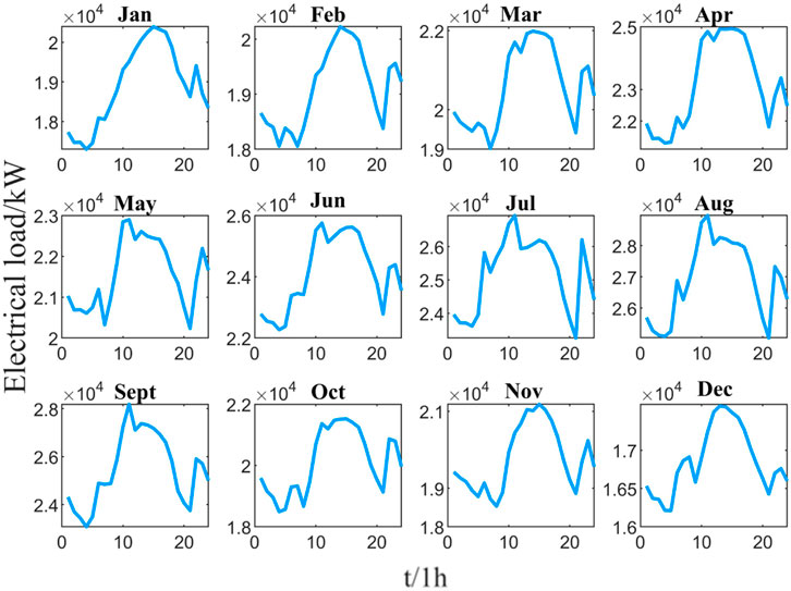
FIGURE 1. Monthly average electric daily load distribution chart.

Firstly, the average monthly electric load distribution series under different months is obtained by taking the average value of parallel load points of the load series under different load days in the same month. Secondly, the obtained daily average electric load distribution series are then compared two by two using grey correlation analysis to form a correlation coefficient matrix $D_{\alpha }$ between different months of the same load with correlation coefficient ${\xi }_{\alpha }\left(i,j\right)$, where $i$ and $j$ are the number of sample series. The variance is used to portray the degree of volatility of the series, and the correlation coefficient is used to portray the similarity between the series. The variance of the daily average load series of different months is used to make the first-order difference, forming the variance first-order difference matrix $D_{\beta }$, and the correlation coefficient is ${\xi }_{\beta }\left(i,j\right)$. The smaller the value in the matrix, the more similar the degree of volatility between the two series is. Finally, the correlation thresholds of the parameters in the above matrix are selected separately to classify the multivariate load similar fluctuation fluctuation set, and the solution flow chart is shown in Figure 2.

FIGURE 2

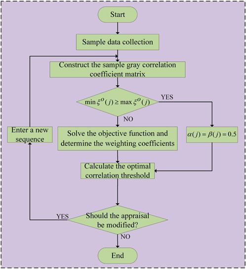
FIGURE 2. Flow chart of correlation coefficient threshold selection.

The correlation threshold ${\xi }^o\left(j\right)$ is actually the final criterion for the attribution of the sample to be examined. If the value of ${\xi }^o\left(j\right)$ is low, association misclassification will occur, i.e., sequences that are not originally part of the fluctuation set are classified, and the lower the value of ${\xi }^o\left(j\right)$, the higher the probability of misclassification. Conversely, if the value of ${\xi }^o\left(j\right)$ is high, the higher the probability of fault omission, the sequence that should have been classified into the fluctuation set is not classified in, and the higher the value of ${\xi }^o\left(j\right)$, the higher the probability of omission. We write down the minimum correlation threshold corresponding to the smallest correlation of the sequence as $\min {\xi }^o\left(j\right)$. Therefore, the maximum correlation threshold corresponding to the largest correlation is written down as $\max {\xi }^o\left(j\right)$. The best value of the correlation threshold ${\xi }^o\left(j\right)op$ should satisfy the following conditions.

$\min {\xi }^o\left(j\right)<{\xi }^o\left(j\right)op<\max {\xi }^o\left(j\right),\min {\xi }^o\left(j\right)<\max {\xi }^o\left(j\right)(1)$

$\min {\xi }^o\left(j\right)={\xi }^o\left(j\right)op=\max {\xi }^o\left(j\right),\min {\xi }^o\left(j\right)=\max {\xi }^o\left(j\right)(2)$

${\xi }^o\left(j\right)op=\alpha \left(j\right)\min {\xi }^o\left(j\right)+\beta \left(j\right)\max {\xi }^o\left(j\right),\min {\xi }^o\left(j\right)>\max {\xi }^o\left(j\right)(3)$

Where $\alpha \left(j\right)$ and $\beta \left(j\right)$ are weighting factors, $0\le \alpha \left(j\right)\le 1$, $0\le \beta \left(j\right)\le 1$, $\alpha \left(j\right)+\beta \left(j\right)=1$.

Let the minimum correlation of the sequence $j$ be $E_w\left(j\right)$ and the maximum correlation be $E_l\left(j\right)$. Establish the objective function on the sequence.

$E\left(\alpha \left(j\right),\beta \left(j\right)\right)=E_w\left(j\right)+E_l\left(j\right)(4)$

Search for $\alpha \left(j\right)$ and $\beta \left(j\right)$ when this objective function is minimized, and find the corresponding correlation threshold, which we call the best correlation threshold at this time, and denote as ${\xi }^o\left(j\right)op$.

4 K-means clustering method for each fluctuation set sequence

4.1 Gray correlation analysis method

Electricity, heat and cold loads in IES have strong correlation for meteorological factors, and the usual prediction method is to artificially and subjectively select several meteorological factors as inputs, which does not seem to be logically sufficiently justified. Therefore, before carrying out multi load prediction of the regional integrated energy system, the various types of loads and the correlation strength between them and meteorological factors should be analyzed and screened, so as to analyze the coupling characteristics among electric, heat and cold loads, as well as the impact of each influencing factor on the multi loads.

GRA compensates for the shortcomings caused by the use of mathematical and statistical methods for systematic analysis. GRA is a multi-factor statistical analysis method, and its basic idea is to determine whether the association is strong or not based on the similarity of the geometry of the series curves. The closer the curves are to the response series, the greater the degree of association between them, and vice versa. The GRA method is suitable for analyzing the nonlinear relationship between multiple loads and influencing factors, which can largely reduce the loss due to information asymmetry, and this method does not need a large number of data sets as the basis, the calculation is small and fast, and there is no discrepancy between quantitative results and qualitative analysis results. Therefore, in this paper, GRA is selected to quantitatively analyze the degree of influence of meteorological factors on the multiplicative load, and the meteorological factors that have the greatest influence on the multiplicative load are selected as the influence factors to analyze the correlation between each influence factor and the multiplicative load.

4.2 Multivariate load and meteorological factor correlation analysis

The correlation coefficient and the correlation degree of the GRA method are two key parameters used to measure the correlation, and the magnitude of the correlation degree can visually reflect the degree of association between two factors, which are calculated by the following equations.

${\xi }_i=\frac{\underset{i}{\min }\underset{k}{\min }\left|x_0\left(k\right)-x_i\left(k\right)\right|+\rho \underset{i}{\max }\underset{k}{\max }\left|x_0\left(k\right)-x_i\left(k\right)\right|}{\left|x_0\left(k\right)-x_i\left(k\right)\right|+\rho \underset{i}{\max }\underset{k}{\max }\left|x_0\left(k\right)-x_i\left(k\right)\right|}(5)$

${\gamma }_i=\frac{1}{n}{\displaystyle \sum }_{k=1}^n{\xi }_i\left(k\right)(6)$

Where $x_0$ is the normalized weather factor sequence, $x_i$ is the normalized load sequence, $\rho$ is the resolution coefficient, generally taken as 0.5, $n$ is the length of the sequence.

The correlation between the multiple loads of the integrated regional energy system and each meteorological influencing factor is analyzed. Let the sequence of electrical, heat and cold loads and each meteorological influence form the following matrix.

Based on the load prediction priorities derived from the above correlation analysis for multivariate loads, the NWP strongly correlated features are used as input for k-means clustering to classify load scenarios, and the BI-LSTM network is trained separately for each load scenario set for sub-scenario set prediction modeling.

$X_s={\left[\begin{array}{c}\begin{array}{c}\begin{array}{c}\begin{array}{c}{x}_E\\ x_H\end{array}\\ x_C\\ \begin{array}{l}{x}_{\mathrm{T}\mathrm{e}\mathrm{m}\mathrm{p}}\\ x_{HUM}\end{array}\end{array}\\ x_{WVEL}\\ x_{WD}\\ x_{GHI}\end{array}\\ x_{\mathrm{P}W}\\ x_{Dp}\\ \begin{array}{l}{x}_{atm}\\ x_{CT}\end{array}\end{array}\right]}^T={\left[\begin{array}{cccc}{x}_E\left(1\right)& x_E\left(2\right)& \cdots & x_E\left(n\right)\\ x_H\left(1\right)& x_H\left(2\right)& \cdots & x_H\left(n\right)\\ x_C\left(1\right)& x_C\left(2\right)& \cdots & x_C\left(n\right)\\ x_{\mathrm{T}\mathrm{e}\mathrm{m}\mathrm{p}}\left(1\right)& x_{\mathrm{T}\mathrm{e}\mathrm{m}\mathrm{p}}\left(2\right)& \cdots & x_{\mathrm{T}\mathrm{e}\mathrm{m}\mathrm{p}}\left(n\right)\\ x_{HUM}\left(1\right)& x_{HUM}\left(2\right)& \cdots & x_{HUM}\left(n\right)\\ x_{WVEL}\left(1\right)& x_{WVEL}\left(2\right)& \cdots & x_{WVEL}\left(n\right)\\ x_{WD}\left(1\right)& x_{WD}\left(2\right)& \cdots & x_{WD}\left(n\right)\\ x_{GHI}\left(1\right)& x_{GHI}\left(2\right)& \cdots & x_{GHI}\left(n\right)\\ x_{\mathrm{P}W}\left(1\right)& x_{\mathrm{P}W}\left(2\right)& \cdots & x_{\mathrm{P}W}\left(n\right)\\ x_{Dp}\left(1\right)& x_{Dp}\left(2\right)& \cdots & x_{Dp}\left(n\right)\\ x_{atm}\left(1\right)& x_{atm}\left(2\right)& \cdots & x_{atm}\left(n\right)\\ x_{CT}\left(1\right)& x_{CT}\left(2\right)& \cdots & x_{CT}\left(n\right)\end{array}\right]}^T(7)$

Where $x_E$ is electrical load, $x_H$ is heat load, $x_C$ is cold load, $x_{\mathrm{T}\mathrm{e}\mathrm{m}\mathrm{p}}$ is temperature, $x_{HUM}$ is relative humidity, $x_{WVEL}$ is wind speed, $x_{WD}$ is wind direction, $x_{GHI}$ is irradiance, $x_{PW}$ is rainfall availability, $x_{Dp}$ is dew point, $x_{atm}$ is atmospheric pressure, and $x_{CT}$ is cloud type.

5 Multivariate load prediction model

5.1 LSTM neural network prediction model

LSTM is an improved model of Recurrent Neural Network (RNN), which solves the gradient disappearance and explosion problems of RNN, enabling the network to effectively handle long-term time series data, improving the ability to handle samples with long time series intervals or delays, as well as the ability to handle non-linear data (Hongbo et al., 2022). The network structure of a typical RNN is shown in Figure 3. $x_t$ is the input, $h_t$ is the output, $c_t$ is the memory state, $A$ is the neural network module. The key is that it can be used to connect previous information to the current task, and to interact with information by stacking multiple neural networks, passing each neural network module corresponding information to the next one. However, the disadvantage is that as the network is extended, the distance between the relevant information and the current predicted location gradually increases, which makes the RNN lose the ability to learn information that is connected so far.

FIGURE 3

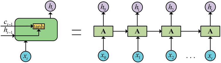
FIGURE 3. Single RNN hidden layer unit expansion structure diagram.

LSTM can learn long-term dependent information, the key of which is the transfer of cell states, and it has the same repetitive way as RNN, but redesigned memory units while retaining the original structure of RNN, The LSTM sets up three control gates, input gate $i_t$, output gate $o_t$, and forgetting gate $f_t$, which are used to select the correction parameters of the error function of the memory feedback with gradient descent, optimizing the weights of the self-loop and keeping the dynamic change of the weights (Fulong et al., 2022), the architecture is shown in Figure 4.

FIGURE 4

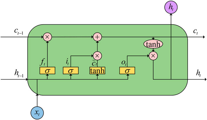
FIGURE 4. LSTM architecture.

As shown in Figure 3, the output value $h_{t-1}$ and the current moment input value $x_t$ passed through the forgetting gate from the implicit layer of the previous moment, the forgetting gate reads the above information and outputs a value between 0 and 1 to each of the data in the cell state $c_{t-1}$. 1 means “complete retention” and 0 means “complete forgetting.” Therefore, the forgetting gate can filter the previous data and discard the useless information. The calculation formula is as follows.

$f_t=\sigma \left(W_f\cdot \left[h_{t-1},x_t\right]+b_f\right)(8)$

Where $W_f$ and $b_f$ are the weight matrix and bias vector in the forgetting gate, respectively, $\sigma$ is the activation function, and the sigmoid function is used.

The new information is then subjected to a sigmoid function to determine the data that needs to be input into the memory cell, while a new candidate state ${\stackrel{\sim }{c}}_t$ is constructed through A. The calculation formula is as follows.

$i_t=\sigma \left(W_i\cdot \left[h_{t-1},x_t\right]+b_i\right)(9)$

${\stackrel{\sim }{c}}_t=\tanh \left(W_c\cdot \left[h_{t-1},x_t\right]+b_c\right)(10)$

Where $W_i$ and $b_i$ are the weight matrix and bias vector in the input gate, respectively, $W_c$ and $b_c$ are the weight matrix and bias vector in the cell state, respectively.

Then, update the cell state, first multiply the old state $c_{t-1}$ and $f_t$ to complete the screening of useless information to delete, and then sum up the product of the calculated result $i_t$ and the new cell state value ${\stackrel{\sim }{c}}_t$ with the input gate, then get the current moment cell state value, the calculation formula is as follows.

$c_t=f_t{c}_{t-1}+i_t{\stackrel{\sim }{c}}_t(11)$

In addition, the implied layer data values $h_t$ passed to the next moment are obtained using the new cell states ${\stackrel{\sim }{c}}_t$ processed by the $\tanh$ function and the data $o_t$ classified by the sigmoid function, the calculation formula is as follows.

$o_t=\sigma \left(W_o\left[h_{t-1},x_t\right]+b_o\right)(12)$

$h_t=o_t*\tanh \left(c_t\right)(13)$

Where $W_o$ and $b_o$ are the weight matrix and bias vector in the output gate, respectively.

5.2 BI-LSTM prediction model

Both RNN and LSTM can only predict the output of the next moment based on the temporal information of the previous moment, but the output of the current moment is not only related to the previous state, but also may be related to the future state. BI-LSTM is a combination of a forward LSTM and a backward LSTM, and its architecture is shown in Figure 5. It can be viewed as a two-layer neural network, with the first layer serving as the starting input for the series from the direction of the input, and the second layer serving as the starting input from the direction of the output.

FIGURE 5

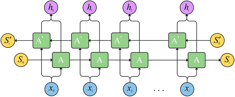
FIGURE 5. BI-LSTM architecture.

To splice and combine the backward-conducted information vector $\left[S_0^{\prime },S_1^{\prime },\cdots ,S_t^{\prime }\right]$ with the forward-conducted information vector $\left[S_0,S_1,\cdots ,S_t\right]$, so that the whole prediction process can take into account the bi-directional information, deepen the understanding of data features, and thus improve the prediction accuracy, and its splicing and combination structure is shown in Figure 6.

FIGURE 6

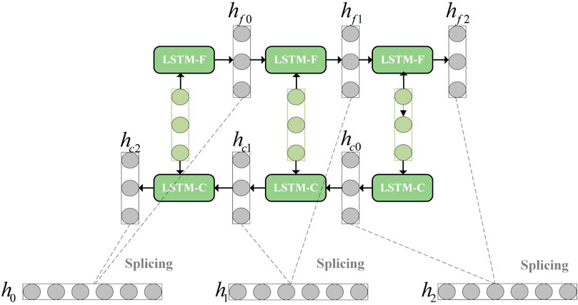
FIGURE 6. BI-LSTM bi-directional conductive splicing combinatorial architecture.

5.3 Step-by-step prediction of multiple loads

The prediction priority of the multiple loads in the IES can be determined based on the cumulative correlation coefficient ${\phi }_i$. Take electric load as an example, select electric load as the benchmark, sum up the correlations of heat, cold and two loads for electric load to get the cumulative correlation coefficients ${\phi }_1$ of hot and cold loads for electric load, and then select heat and cold loads as the benchmark respectively to get the cumulative correlation coefficients ${\phi }_2$ and ${\phi }_3$ of the selected loads relative to the other two loads. The smaller the value of cumulative correlation, the less coupling with other loads, and vice versa. Then, the priority of multiple load prediction can be determined according to the increasing order of the cumulative correlation coefficients.

On the basis of the load prediction method of the above priority, the idea of prioritized step-by-step prediction is adopted, as the electrical and cold loads have the weakest correlation for heat loads, followed by electrical and heat loads for cold loads, and again by heat and cold loads for electrical loads. Accordingly, the predicted heat load can be considered first, and the predicted heat load is first used as input combined with the NWP characteristics of the strong correlation of the cold load and the load mean value series of the first 16 time points of the prediction period for the prediction of the cold load in the set of sub-load sc. Secondly, the predicted hot load and cold load are used as the input combined with the strong correlation NWP characteristics of the electric load and the load mean value series of the first 16 time points of the prediction period to predict the electric load. Finally the overall prediction results of the multiple loads are obtained, where the overall prediction process is shown in Figure 7.

FIGURE 7

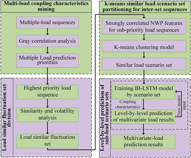
FIGURE 7. Flow chart of multivariate load data prediction.

6 Example analysis

6.1 Data source

Example load data from Campus Metabolism for the Temp campus of Arizona State University from 1 January 2019 at 00:00 h to 31 December 2019 at 24:00 h for electricity, heat and cold (Arizona State University, 2022), Meteorological data were obtained from the National Climatic Resources website for the Tempe campus location (U.S. Department of Energy, 2022), including temperature, relative humidity, wind speed, wind direction, irradiance, rainfall availability, dew point, atmospheric pressure, and cloud type, at 15-min sampling intervals.

6.2 Model evaluation metrics

In this paper, Root Mean Square Error (RMSE), Mean Absolute Percentage Error (MAPE) and Mean Absolute Error (MAE) are selected as the evaluation indexes, and the expressions of the specific evaluation indexes are as follows.

$RMSE=\sqrt{\frac{1}{N}{\displaystyle \sum }_{t=1}^N{\left(y_t-y_t^{\prime }\right)}^2}(14)$

$MAPE=\frac{1}{N}{\displaystyle \sum }_{t=1}^N\left|\frac{y_t^{\prime }-y_t}{y_t}\right|\times 100\%(15)$

$MAE=\frac{1}{N}{\displaystyle \sum }_{t=1}^N\left|y_t^{\prime }-y_t\right|(16)$

Where $y_t$ is the actual value, $y_t^{\prime }$ is the predicted value, $t$ is the sampling moment, $N$ is the sample size.

6.3 Load scenario set division results

Based on the results of gray correlation degree analysis in this paper, the highest priority electric load is used as the basis for the division of load scenarios, and the similar fluctuating sets of load for 12 months of a year are obtained according to the similarity and fluctuation division of load sequences. Among them, the load of a year is divided into four sets by month as shown in Table 1.

TABLE 1

TABLE 1. Results of load similar fluctuation set division.

The correlation degree analysis of the strongly correlated NWP features of the multivariate loads is required before the load scenario set division, based on the results of the gray correlation degree analysis, as shown in Table 2. The results show that the strength of the correlation between each meteorological influence factor and the electric, heat and cold loads varies, so it is necessary to correspond the meteorological influence factors to the load types in a reasonable way when prediction.

TABLE 2

TABLE 2. Correlation analysis between multivariate load and NWP characteristics.

Based on the results of the strong correlation NWP fluctuation analysis of multiple loads, the NWP features of each load are input into the k-means clustering model to obtain the clustering cluster division of each load under each fluctuation set and train the BI-LSTM model separately for each cluster to realize the sub-load scenario set prediction.

6.4 Multiple load prediction priorities

Since the paper is mainly based on the coupling characteristics of multiple loads to prioritize the single load sequence for load prediction, the coupling relationship of multiple loads obtained based on gray correlation analysis is shown in Table 3. The influence of day type information and meteorological influences on the degree of load coupling is taken into account. For the first predicted heat load, six meteorological factors with the highest correlation are selected for prediction, and then the cold load is predicted iteratively using the predicted heat load data and the corresponding meteorological influences on the cold load. And so on, ensuring that each load forecast from the second priority load forecast onwards iterates over the previous load forecast results and the newly added meteorological impact factors. The following results can be obtained from Table 3: ${\phi }_1$ = 1.4255、 ${\phi }_2$ = 1.3561、 ${\phi }_3$ = 1.3596.

TABLE 3

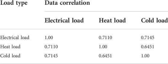
TABLE 3. Correlation analysis between multiple loads.

6.5 Analysis of experimental results

6.5.1 Prediction results for load scenario set partitioning

According to the idea of differentiated priority prediction, the heat load is first predicted. Prediction method 1: A sequence of meteorological factors strongly correlated with the heat load and a sequence of heat load history data are used as inputs, where the input meteorological factors are forecast data for the forecast period and the heat load history data are measured data for the 4 hours before the forecast period. Prediction method 2: Extract the strongly correlated meteorological element sequences within the similar fluctuation set with time interval of 1 hour by day as the input of k-means clustering model for load scenario set division, and train the model separately for prediction by load scenario set according to the division result, at which time the input is the same as prediction method 1. In order to highlight the effect of clustering division, 2 days per month are selected for load prediction for similar fluctuation concentration at this time, and the load prediction results for 6 days are obtained, as shown in Figure 8, which shows that the prediction curve of the proposed prediction method in this paper is closer to the actual value curve.

FIGURE 8

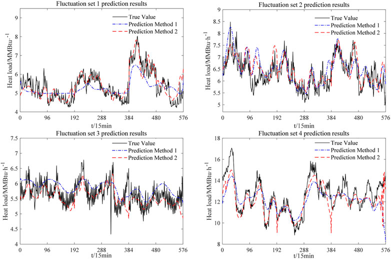
FIGURE 8. Heat load prediction results.

Among them, the error evaluation indexes of the prediction results are shown in Table 4. The errors obtained by prediction method two based on load scenario set division are smaller compared with those obtained by prediction method 1, in which MAPE is reduced by 1.59% on average, RMSE is reduced by 0.14 MMBtu·h⁻¹ on average, and MAE is reduced by 0.11 MMBtu·h⁻¹ on average.

TABLE 4

TABLE 4. Comparison of heat load prediction results.

6.5.2 Prediction results for load scenario set partitioning

Prediction results base on heat load, the coupling characteristics are considered for the prediction of cold load taking into account the priority of multiple load prediction. In this case, due to the consideration of the coupling characteristics, the prediction results of the heat load, as well as the strongly correlated meteorological characteristic series and the actual cold load series of the first 4 hours of the prediction period are used as inputs. The prediction method 1 that directly predicts considering the coupling characteristics, the prediction method 2 that divides the set of load scenes without considering the coupling characteristics, and the prediction method 3 that considers both the coupling characteristics and the division of the set of load scenes are obtained. The prediction results are shown in Figure 9.

FIGURE 9

FIGURE 9. Cold load prediction results.

A comparison of the results of multiple prediction methods is shown in Table 5, where the prediction method 2 without considering the coupling characteristics is less effective, with the highest average absolute percentage error reaching 10.26%, prediction method 3 has the smallest prediction error because it considers the coupling characteristics of multiple loads and divides the set of load scenarios. Compared with the prediction method 1, the MAPE was reduced by 2.06%, RMSE by 278.93 Ton, and MAE by 188.82 Ton on average, compared to prediction Method 2, MAPE is reduced by 2.98% on average, RMSE by 219.30 Ton on average, and MAE by 389.47 Ton on average.

TABLE 5

TABLE 5. Comparison of cold load prediction results.

According to the above obtained heat and cold load prediction values, the electric load is predicted by considering the coupling characteristics. In this case, the electrical load forecast inputs include the forecasted hot and cold loads as well as strongly correlated meteorological characteristics and measured electrical load data for the first 4 hours of the forecast period. As the coupling characteristics and load scenario set division are considered, the same three prediction modes as the cold load are obtained, and the prediction results are shown in Figure 10. It can be seen that the average absolute percentage error of prediction method 3 decreases by 0.55% and 0.66% on average compared with prediction method 1 and prediction method 2. Respectively, which is due to the fact that prediction method 3 takes into account the characteristics of multi-energy coupling in IES and uses the remaining two loads as references, which in turn improves its prediction accuracy.

FIGURE 10

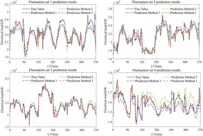
FIGURE 10. Electrical load prediction results.

Due to the consideration of multivariate load coupling characteristics and the division method of load scenario set, the prediction results of prediction method 3 have less prediction error than the other two prediction methods, This is mainly reflected in the peak and valley hours of the load, and the prediction method 3 is more reflective of the actual load variation, which reflects that the prediction method considering the division of load scenarios and taking into account the coupling characteristics is more practical for IES multi load prediction. The electrical load forecast errors are shown in Table 6. Although the electric load prediction errors obtained by the three prediction methods are not significantly different, the prediction errors obtained by the prediction method considering coupling characteristics and load scenario set division are smaller.

TABLE 6

TABLE 6. Comparison of electrical load prediction results.

7 Conclusion

1) In order to improve the accuracy of multivariate load prediction, this paper proposes a similar fluctuation feature set partitioning method considering the coupling characteristics of multivariate loads. By studying the coupling strength between multiple types of energy in IES to determine the prediction priority of multiple loads, the interactive coupling between electric, heat and cold loads is fully considered. The NWP features with strong correlation with multiple loads are obtained by gray correlation analysis, and k-means clustering is performed using the inter-set NWP as input, and fine-grained modeling is performed for each cluster. The analysis of the arithmetic examples leads to the following main conclusions.

2) Based on the load similar fluctuation set division method proposed in this paper, four fluctuation sets are obtained. The load fluctuation types within each fluctuation set are similar, and the load scenario set is divided based on the k-means clustering model for each load similar fluctuation set. And according to the results of the above analysis, the priority of load forecasting is considered, and the heat load, cold load and electric load are predicted step by step according to the fluctuation set and load scenario set respectively.

3) The prediction results based on multiple prediction methods show that the average absolute percentage errors of electric, heat, and cold loads are 2.85%, 5.22%, and 4.06% for the prediction methods considering the division of load scenario sets and coupling characteristics in the overall prediction results of four load similar fluctuation sets. The average absolute percentage error is reduced by 0.66%, 1.53% and 2.99% respectively compared to the prediction method considering only load scenarios, compared with the prediction method without considering load scenes, its average absolute percentage errors are reduced by 0.55%, 1.53%, and 2.07%, respectively, which verifies the effectiveness of the prediction method considering the division of load scenes set and coupling characteristics.

With the popularity of IES and the development of interconnected IES, the division of IES types can be considered in the subsequent study so as to realize the collaborative prediction among multiple IESs.

Data availability statement

The original contributions presented in the study are included in the article/supplementary material, further inquiries can be directed to the corresponding author.

Author contributions

MY: Writing—original draft. DL: Validation, Visualization. XS: Methodology. JW: Software, Supervision. YC: Data curation.

Funding

This work was supported by National Key R&D Program of China [Technology and application of wind power/photovoltaic power prediction for promoting renewable energy consumption (2018YFB0904200)].

Conflict of interest

The authors declare that the research was conducted in the absence of any commercial or financial relationships that could be construed as a potential conflict of interest.

Publisher’s note

All claims expressed in this article are solely those of the authors and do not necessarily represent those of their affiliated organizations, or those of the publisher, the editors and the reviewers. Any product that may be evaluated in this article, or claim that may be made by its manufacturer, is not guaranteed or endorsed by the publisher.

References

Abhishek, S., and Sachin, K. J. (2022). A novel seasonal segmentation approach for day-ahead load forecasting. Energy 257, 124752. doi:10.1016/j.energy.2022.124752

CrossRef Full Text | Google Scholar

Arizona State University (2022). Campus metabolism. https://cm.asu.edu (Accessed August 11, 2022).

Google Scholar

Fulong, Y., Wenju, Z., Mostafa, A. G., Yang, S., and Wanqing, Z. (2022). An integrated D-CNN-LSTM approach for short-term heat demand prediction in district heating systems. Energy Rep. 8 (13), 98–107. doi:10.1016/j.egyr.2022.08.087

CrossRef Full Text | Google Scholar

Haohan, T., Zhisheng, Z., and Daolin, Y. (2021). Research on multi-load short-term forecasting of regional integrated energy system based on improved LSTM. Proc. CSU-EPSA. 33 (9), 130–137. doi:10.19635/j.cnki.csu-epsa.000726

CrossRef Full Text | Google Scholar

Hongbo, R., Qifen, L., Qiong, W., Chunyan, Z., Zhenlan, D., and Jie, C. (2022). Joint forecasting of multi-energy loads for a University based on copula theory and improved LSTM network. Energy Rep. 8 (10), 605–612. doi:10.1016/j.egyr.2022.05.208

CrossRef Full Text | Google Scholar

Jinpeng, C., Zhijian, H., and Weinan, C. (2021). Load prediction of integrated energy system based on combination of quadratic modal decomposition and deep bidirectional long short-term memory and multiple linear regression. Autom. Electr. Power Syst. 45 (13), 85–94. 10. 7500/AEPS20200829004.

Google Scholar

Jixiang, L., Qipei, Z., Zhihong, Y., Mengfu, T., Jinjun, L., and Hui, P. (2019). Short-term load forecasting method based on CNN-LSTM hybrid neural network model. Autom. Electr. Power Syst. 43 (08), 131–137. doi:10.7500/AEPS20181012004

CrossRef Full Text | Google Scholar

Jizhong, Z., Hanjiang, D., Shenglin, L., Ziyu, C., and Tengyan, L. (2021). Review of data-driven load forecasting for integrated energy system. Proc. CSEE 41 (23), 7905–7924. doi:10.13334/j.0258-8013.pcsee.202337

CrossRef Full Text | Google Scholar

Jizhong, Z., Hanjiang, D., Weiye, Z., Shenglin, L., Yanting, H., and Lei, X. (2022). Review and prospect of data-driven techniques for load forecasting in integrated energy systems. Appl. Energy 321, 119269. doi:10.1016/j.apenergy.2022.119269

CrossRef Full Text | Google Scholar

Kai, Z., Jian, F., Jianhua, L., Xinlei, B., Feixiang, G., Zudong, L., et al. (2022). Power consumption behavior pattern classification based on fuzzy C&hybull;mean clustering algorithm. Power Demand Side Manag. 24 (3), 98–103. doi:10.3969/j.issn.1009-1831.2022.03.016

CrossRef Full Text | Google Scholar

Luiz, F., and Afshin, A. (2015). Short-term forecasting of the abu dhabi electricity load using multiple weather variables. Energy Procedia 75, 3014–3026. doi:10.1016/j.egypro.2015.07.616

CrossRef Full Text | Google Scholar

Mao, Y., Chaoyu, S., and Huiyu, L. (2020). Day-ahead wind power forecasting based on the clustering of equivalent power curves. Energy 218, 119515. doi:10.1016/j.energy.2020.119515

CrossRef Full Text | Google Scholar

Mao, Y., Meng, Z., Dawei, H., and Xin, S. (2022). A composite framework for photovoltaic day-ahead power prediction based on dual clustering of dynamic time warping distance and deep autoencoder. Renew. Energy 194, 659–673. doi:10.1016/j.renene.2022.05.141

CrossRef Full Text | Google Scholar

Mukhopadhyay, P., Mitra, G., Banerjee, S., and Mukherjee, G. (December 2017). “Electricity load forecasting using fuzzy logic: Short term load forecasting weather parameter,” in Proccedings of the 2017 7th international conference on power systems (ICPS), Pune, India 812–819. doi:10.1109/ICPES.2017.8387401

CrossRef Full Text | Google Scholar

Nantian, H., Qingkui, H., Jiajin, Q., Qiankun, H., Rijun, W., Guowei, C., et al. (2022). Multinodes interval electric vehicle day-ahead charging load forecasting based on joint adversarial generation. Int. J. Electr. Power & Energy Syst. 143, 108404. doi:10.1016/j.ijepes.2022.108404

CrossRef Full Text | Google Scholar

Qingkai, S., Xiaojun, W., Yizhi, Z., Fang, Z., Pei, Z., and Wenzhong, G. (2021). Multiple load prediction of integrated energy system based on long short-term memory and multi-task learning. Autom. Electr. Power Syst. 45 (5), 63–70.doi:10.7500/AEPS20200306002

CrossRef Full Text | Google Scholar

Tang, Y., Liu, H., Xie, Y., Zhai, J., and Wu, X. (2019). Short-term forecasting of electricity and gas demand in multi-energy system based on RBF-NN model. IEEE Int. Conf. Energy Internet (ICEI), 542–547. doi:10.1109/ICEI.2019.00102

CrossRef Full Text | Google Scholar

U.S. Department of Energy (2022). NSEDB:National solar radiation database. https://nsrdb.nrel.gov/ (Accessed August 11, 2022).

Google Scholar

Valery, S., Evgeny, B., Dmitry, S., and Bin, Z. (2022). Current state of research on the energy management and expansion planning of integrated energy systems. Energy Rep. 8, 10025–10036. doi:10.1016/j.egyr.2022.07.172

CrossRef Full Text | Google Scholar

Wang, X., Wang, S., Zhao, Q., Wang, S., and Fu, L. (2021). A multi-energy load prediction model based on deep multi-task learning and ensemble approach for regional integrated energy systems. Int. J. Electr. Power & Energy Syst. 126 (A), 106583. doi:10.1016/j.ijepes.2020.106583

CrossRef Full Text | Google Scholar

Wei, W., Lin, X., Jierui, X., Chang, L., Xiaofeng, J., and Kai, L. (2022). Coupled dispatching of regional integrated energy system under an electric-traffic environment considering user equilibrium theory. Energy Rep. 8, 8939–8952. doi:10.1016/j.egyr.2022.07.008

CrossRef Full Text | Google Scholar

Wu, Y., Liang, X., Huang, T., Lin, Z., Li, Z., and Hossain, M. (2021a). A hierarchical framework for renewable energy sources consumption promotion among microgrids through two-layer electricity prices. Renew. Sustain. Energy Rev. 145, 111140. doi:10.1016/j.rser.2021.111140

CrossRef Full Text | Google Scholar

Wu, Y., Lin, Z., Liu, C., Chen, Y., and Uddin, N. (2021b). A demand response trade model considering cost and benefit allocation game and hydrogen to electricity conversion. IEEE Trans. Ind. Appl. 58, 2909–2920. doi:10.1109/TIA.2021.3088769

CrossRef Full Text | Google Scholar

Xiaobo, Z., and Jianzhou, W. (2018). A novel decomposition-ensemble model for forecasting short-term load-time series with multiple seasonal patterns. Appl. Soft Comput. 65, 478–494. doi:10.1016/j.asoc.2018.01.017

CrossRef Full Text | Google Scholar

Xuexiang, L., Haowen, L., Xudong, Z., Zhonghe, H., Yu, C., and Min, Y. (2022). A novel neural network and grey correlation analysis method for computation of the heat transfer limit of a loop heat pipe (LHP). Energy 259, 124830. doi:10.1016/j.energy.2022.124830

CrossRef Full Text | Google Scholar

Yang, M., Zhang, L., Cui, Y., Zhou, Y., Chen, Y., and Yan, G. (2019). Investigating the wind power smoothing effect using set pair analysis. IEEE Trans. Sustain. Energy 11, 1161–1172. doi:10.1109/TSTE.2019.2920255

CrossRef Full Text | Google Scholar

Yingjun, W., Zhiwei, L., Chengjun, L., Tao, H., Yuyang, C., Yingtao, R., et al. (2022). Resilience enhancement for urban distribution network via risk-based emergency response plan amendment for ice disasters. Int. J. Electr. Power & Energy Syst. 141, 108183. doi:10.1016/j.ijepes.2022.108183

CrossRef Full Text | Google Scholar