Hybrid kernel search and particle swarm optimization with Cauchy perturbation for economic emission load dispatch with valve point effect

Due to growing concerns over environmental protection, economic and environmentally responsible power dispatching has become a hot topic in the field of power system control. Multi-objective optimization minimizes fuel costs and pollution emissions without violating operational constraints. To solve this problem, the MOP is decomposed into individual objects via the weighted sum method, and Newton’s method is used to tackle equality constraints iteratively. To this end, a hybrid algorithm (HKSOPSO-CP) based on kernel search optimization (KSO) and particle swarm optimization (PSO) with Cauchy perturbation is proposed in this paper. An experiment with 23 CEC benchmark functions shows that HKSOPSO-CP offers better performance compared with various popular algorithms proposed in recent years. When employed to solve the IEEE standard economic emission dispatch (EED) problems with 6, 10, 40, and 110 units, the proposed HKSOPSO-CP algorithm produces results indicating a better trade-off between the objectives relating to fuel costs and emissions compared to other algorithms that have recently been reported on in the literature.

1 Introduction

The goal of economic dispatch (ED) is to schedule power generation to minimize the cost of producing electricity within the confines of operational constraints, such as the demand load and transmission loss. Decision makers in energy fields need effective hybrid models in order to reduce the cost of operations as much as possible (Ge et al., 2022a; Ge et al., 2022b; Chen, 2022). Even minor improvements in the operation of power plants can bring substantial economic benefits. Furthermore, thermal power plants inevitably emit a large amount of pollution during the operation of power systems, which has become a critical issue with increasing concerns over global warming. Therefore, the problem of simultaneous combined minimization of fuel costs and pollutant emissions, known as the economic emission dispatch (EED) problem, has become a research focus.

With people’s increasing awareness of pollutant emissions, the economic emission dispatch problem (EED), which seeks to minimize fuel costs and pollution, has been a growing concern. The EED problem represents a multi-objective optimization problem (MOP) (El-Keib and Ding, 1994). The aim in solving it is to find the best possible power distribution for each generator without violating the relevant constraints. In order to solve this type of problem, various techniques have been developed.

Optimization methods can be regarded as falling into various classes, including deterministic, stochastic, and evolutionary (Wang et al., 2022a). Traditional methods attempt to guarantee exact solutions (Zhang et al., 2022a), while in contrast, recent evolutionary methods cannot guarantee the identification of trustworthy optimal solutions, and it is regarded as sufficient to return solutions only satisfying local optima (Cao et al., 2022a). Recently, many studies have been conducted to solve the EED problem. There is a growing interest in many modern random-based metaheuristic algorithms (MAs), because they do not need any derivative information or gradient information in the search process (Jadhav et al., 2013); these methods include particle swarm optimization (PSO) (Cao et al., 2020; Lin et al., 2022), the colony predation algorithm (CPA) (Tu et al., 2021), hunger games search (HGS) (Yang et al., 2021), Harris hawks optimization (HHO) (Heidari et al., 2019), the slime mould algorithm (SMA) (Li et al., 2020a), the weighted mean of vectors (INFO) (Ahmadianfar et al., 2022), and the Runge Kutta optimizer (RUN) (Ahmadianfar et al., 2021), which have yielded great success in a variety of fields, such as feature selection (Hu et al., 2022; Liu et al., 2022), economic emission dispatch (Dong et al., 2021), bankruptcy prediction (Xu et al., 2019; Zhang et al., 2021), train scheduling (Song et al., 2023), image segmentation (Hussien et al., 2022; Yu et al., 2022), multi-objective problems (Hua et al., 2021; Deng et al., 2022a), gate resource allocation (Wu et al., 2020a; Deng et al., 2020), complex optimization problems (Deng et al., 2022b), resource allocation (Deng et al., 2022c), expensive optimization problems (Li et al., 2020b; Wu et al., 2021a), airport taxiway planning (Deng et al., 2022d), robust optimization (He et al., 2020), scheduling problems (Gao et al., 2020; Han et al., 2021; Wang et al., 2022b), and medical diagnosis (Wang et al., 2017) (Chen et al., 2016). Hota et al. (2010) used fuzzy computing to solve EED problems using a modified bacterial foraging algorithm (MBFA). Roy and Bhui used quasi-oppositional teaching learning based optimization (QOTLBO) (Roy and Bhui, 2013) to solve the problem of EED with valve point loading. de Athayde Costa e Silva et al. (2013) used an improved scatter search (ISS) to solve EED problems; experimental results showed that the ISS method achieves a better optimal result than other optimization algorithms.

Yang (Abdelaziz et al., 2016a) proposed the flower pollination algorithm (FPA). This approach can meet the needs of single-objective and multi-objective optimization problems, so it has strong universality in tackling various problems in the domain of power systems. Therefore, Abdelaziz et al. (2016b) used the FPA to solve the EED problem. Simulation results show that the FPA method achieves better results than other methods for various optimization problems, especially for large power systems. Kumar et al. (2012) proposed the Pareto bee colony optimization algorithm and applied it to the standard IEEE 30-bus system to tackle the EED problem. The experimental results were better than those achieved by other multi-objective optimization algorithms. Singh and Dhillon used an opposition-based greedy heuristic search (OGHS) (Singh and Dhillon, 2016) to tackle the power system scheduling problem. In this type of problem, an initial population is randomly generated by means of a uniform distribution, and the inverse solution is generated by means of oppositional learning. The optimal solution is retained for further optimization, which is beneficial to accelerate the convergence rate. Goudarzi et al. (2019) tackled the EED problem using a combination of a genetic algorithm (GA) and particle search optimization (PSO). Hosny et al. (2021) adopted an improved version of the slime mould algorithm (ISMA) to solve the EED problem, enhancing its search capabilities and balancing global and local search. The results showed that, compared with other optimization algorithms, the ISMA method achieves better optimization. Dong et al. proposed a kernel search optimization algorithm (KSO) (Dong and Wang, 2020; Dong et al., 2021) to solve the EED problem. By projecting the function from low-dimensional space to high-dimensional space, the non-linear problem can be transformed into a linear problem. In comparison with other algorithms, better optimal results are obtained.

As mentioned above, the identification of a better multi-objective optimization algorithm is always a research hotspot in the field of power system scheduling optimization. Such improvements take a great deal of effort, and even a small change represents a major improvement in environmental and economic terms. This article proposes an enhanced new metaheuristic for optimization, which uses kernel techniques from the KSO algorithm combined with a PSO algorithm, to tackle the EED problem. The main contributions of this paper can be summarized as follows:

• The local search ability of the KSO algorithm is improved by introducing sociality and self-recognition from the PSO algorithm. The update to the kernel vector in KSO is calculated based on the current velocity and position of the particle instead of via randomization.

• The Cauchy distribution approaches 0 more slowly than the normal distribution, so Cauchy mutation has the better disturbance ability. Cauchy mutation is utilized to update the target position to expand the distribution area of feasible solutions and improve the algorithm’s global optimization performance.

• A hybrid KSO and PSO algorithm with Cauchy perturbation is utilized to solve the EED problem. Moreover, the weighted sum method transforms the multi-objective EED into a single-objective problem, and the Newton–Raphson method handles the power balance constraint.

• The HKSOPSO-CP algorithm is verified by solving EED problem cases involving four electrical systems. It is thereby demonstrated that the proposed algorithms can provide better solutions to EED problems than conventional KSO and other algorithms entered into this comparison.

• Under testing with 23 CEC benchmark functions, the HKSOPSO-CP algorithm outperforms KSO and several other well-known algorithms in accuracy.

The remainder of this article is organized as follows: Section 2 lays out the mathematical model of the EED problem; Section 3 presents the original KSO and PSO algorithms and the Cauchy mutation mechanism, as well as the new HKSOPSO-CP algorithm; Section 4 presents the experimental results and analysis; and Section 5 provides the conclusion.

2 The economic emission dispatch problem

In the EED problem, the objective is to minimize fuel costs while simultaneously minimizing pollutant emissions by identifying the generator schedule that represents the best compromise.

2.1 The objective function

The objective function of the fuel costs can be expressed as follows (Sierpina, 2013):

$C={\displaystyle \sum }_{i=1}^N\left[a_i+b_i{P}_i+c_i{P}_i^2+\left|e_i\sin \left(fi\left(P_i^{\min }-P_i\right)\right)\right|\right](1)$

where C is the fuel cost in the problem to be solved; $a_i$, $b_i$, and $c_i$ represent the cost coefficients for the $i$ th unit; $e_i$ and $f_i$ represent the valve point effect coefficients; $Pi$ represents the power output; and $N$ indicates the number of generating units.

The total emission of pollutants can be defined as follows (Mavrovouniotis and Yang, 2011):

$E={\displaystyle \sum }_{i=1}^N\left[{\alpha }_i+{\beta }_i{P}_i+{\gamma }_i{P}_i^2+{\eta }_i\exp \left({\delta }_i{P}_i\right)\right](2)$

where $E$ is the pollution emission in the problem to be solved, and ${\alpha }_i$, ${\beta }_i$, ${\gamma }_i,{\eta }_i,$ and ${\delta }_i$ represent the emission coefficients of the $i$ th generator.

There are two different objectives in this multi-objective optimization problem. The weighted sum method decomposes the MOP into individual objectives to solve this problem. The method combines conflicting objectives by introducing weight factors. The combined objective function takes the following form (Yaşar and Özyön, 2012):

$F=wC+\gamma \left(1-w\right)E(3)$

where w is the weight factor and $\gamma$ is the scaling factor.

2.2 System constraints

1) Power balance constraints: the total power of all the generators must cover the sum of the load demand and the losses of the real power system (Zhan et al., 2014),

${\displaystyle \sum }_{i=1}^N{P}_i=P_D+P_L,P_L={\displaystyle \sum }_{i=1}^N{\displaystyle \sum }_{j=1}^N{P}_i{B}_{ij}{P}_j+{\displaystyle \sum }_{i=1}^{N}Pi+B_{00},(4)$

where $N$ is the loss coefficient, $B_{ij}$ represents the number of generators, $P_L$ represents the transmission losses, and $P_D$ represents the system load.

2) Power capacity limitation: Each generator’s output must fall within its relative output range (maximum-minimum),

$P_i^{\mathit{min}}\le P_i\le P_i^{\mathit{max}}(5)$

where $P_i^{\mathit{max}}$ and $P_i^{\mathit{min}}$ are the operational limits for the $i$ th generating unit.

The inequality constraint of Eq. 5 can be easily satisfied by setting the upper limit and lower limit in the initialization stage. But the equality constraint of Eq. 4 is usually difficult to satisfy. Therefore, Newton’s method is used to tackle the constraints iteratively:

$P_i=P_i^{\min }+rand\left[\mathrm{0,1}\right]\times \left(P_i^{\max }-P_i^{\min }\right)i=\mathrm{1,2},\dots \dots N-1(6)$

where $P_i$ is the output of the $i$ th generating unit.

It is possible to solve Eq. 4 iteratively for the original output of the Nth generator:

$P_N^{old}=p_D-{\displaystyle \sum }_{i=1}^{N-1}{P}_i(7)$

The transmission loss of the power system $P_L^{old}$ can be expressed in the form of B-matrix coefficients (Zou et al., 2017):

$P_L^{old}={\displaystyle \sum }_{i=1}^N{\displaystyle \sum }_{j=1}^N{P}_i{B}_{ij}{P}_j+{\displaystyle \sum }_{i=1}^n{B}_{0i}{P}_i+B_{00}(8)$

where $P_L^{old}$ is the original output of the $Nth$ generator.

Subsequently, the new output of the Nth generator can be calculated as follows:

$P_N^{new}=P_D-{\displaystyle \sum }_{i=1}^{N-1}{P}_i-P_L^{old}(9)$

The new output of the Nth generator is then substituted into Eq. 8 until the difference between them is less than some minimal value.

The Nth generator $P_N$, following the above steps, is able to fulfill the equality constraint of Eq. 4, but it is uncertain whether its output falls within the feasible domain or not. Therefore, a common penalty function is utilized here as an effective way to address this.

For Eq. 10, an efficient method employing a penalty function is applied to determine whether the output of the Nth generator that satisfies the constraint of Eq. 4 is within the feasible region.

$\stackrel{\sim }{F}=F+\lambda \left[\max \left(P_N^{\min }-P_N,0\right)+\max \left(P_N-P_N^{\max },0\right)\right](10)$

where $\lambda$ is a penalty factor.

3 The principle of the HKSOPSO-CP algorithm

The conventional KSO algorithm and the improved HKSOPSO-CP technique developed using the PSO algorithm and Cauchy perturbation are described in this section.

3.1 Overview of the KSO algorithm

KSO, proposed by Dong (Dong and Wang, 2020) in 2020, is a novel swarm intelligence algorithm whose search strategy is based on the kernel method. KSO was inspired by existing physical or biological MAs, but differs markedly from them: all the MAs mentioned above involve non-linear iterations to approach the optimal values of the target functions, but KSO involves linear iteration via the kernel method. The inspiration is as follows.

The non-linear objective function $y=f\left(x\right)$, $x=\left(x_1,x_2,\dots x_n\right)$ can be converted into a linear one in higher-dimensional space by a mapping function $u=\varphi \left(x\right)$. As the dimensionality of the space increases, the possibility of a non-linear function being transformed into a linear function becomes stronger. This is represented as:

$y=f\left(x\right)=w^T\cdot u+b$

$w=\left(w_1,w_2,\dots w_m\right)$

$u=\left(u_1,u_2,\dots u_m\right)$

where m is the dimensionality of the higher-dimensional space, and $w=\left(w_1,w_2,\dots w_m\right)$ and $u=\left(u_1,u_2,\dots u_m\right)$ are both m-dimensional vectors.

An m-dimensional vector of $a=\left(a_1,a_2,\dots a_n\right)$ is mapped from the n-dimensional vector $w$, that is $w=\varphi \left(a\right)$. The slope of a hyperplane in m dimensions is the direction along which the optimal value lies, denoted by $\varphi \left(a\right)$; then:

$y=f\left(x\right)=w^T\cdot u+b=\phi \left(a\right)\cdot \phi \left(x\right)+b=K\left(a,x\right)+b(11)$

where $K\left(a,x\right)$ is the kernel function.

As a function in a higher-dimensional space, the optimal value is the solution of the lower-dimensional objective function.

The RBF function maps the objective function to an infinitely high-dimensional space (Basu and Basu, 2011) (KSO), which may transform a non-linear function into a linear function. Therefore, the RBF function is used:

$k\left(x,y\right)=\exp \left(\frac{\parallel x-a{\parallel }^2}{\sigma }\right),y=f\left(x\right)=K\left(a,x\right)+b=\exp \left(\frac{\parallel x-a{\parallel }^2}{\sigma }\right)(12)$

The optimization results of the fitted kernel function are considered to approximately represent the minimum of the objective function; these results are converged on by several iterations to bring them close to the best possible result. At the same time, Eq. 12 provides an approximate solution to the optimization problem by a single iteration of the objective function.

The minimum value of the formula is given directly.

$x_{best}\left\{\begin{array}{c}{x}_{\mathit{min}}\sigma <0anda\ge \frac{1}{2}\left(x_{\mathit{min}}+x_{\mathit{max}}\right)\\ x_{\mathit{max}}\sigma <0anda<\frac{1}{2}\left(x_{\mathit{min}}+x_{\mathit{max}}\right)\\ a\sigma >0and{x}_{\mathit{min}}\le a\le x_{\mathit{max}}\\ x_{\mathit{max}}\sigma >0anda>x_{\mathit{max}}\end{array}\right.(13)$

where $x\in \left[x_{\mathit{min}},x_{\mathit{max}}\right]$, and the minimum is $x_{best}$.

Based on Eq. 13, it can be seen that the minimum value $x_{best}$ is at the boundary, or vector a is equivalent to it, corresponding to the low-dimensional pre-image mapped to the high-dimensional hyperplane slope. The vector a is referred to as the kernel vector, which points the searches made in the iterative optimization process in a particular direction. Specifically, it is solved for via Eq. 14.

$\sigma \ln \left(y-b\right)={‖x-a‖}^2={\left(x_1-a_1\right)}^2+{\left(x_2-a_2\right)}^2+...{\left(x_n-a_n\right)}^2(14)$

To solve Eq. 14, posit a random vector $temp1=\left(x_1^{\prime },x_2^{\prime },\dots x_n^{\prime }\right)$; the $i$ th item of the primitive vector x is replaced by the corresponding item of temp1, forming a new vector $\left(x_1,x_2,\dots x_i^{\prime },\dots x_n\right).$ The new vectors form a matrix whose function is $y_i^{\prime }$.

$x^{\prime }=\left(\begin{array}{l}{x}_1^{\prime },x_2,...x_i,...x_n\\ ...\\ x_1,x_2,...x_i^{\prime },...x_n\\ ...\\ x_1,x_2...x_i,...x_n^{\prime }\end{array}\right)$

Then,

$a_{\dot{i}}=\frac{1}{2}\left[x_i+x_j^{\prime }-\sigma \ln \left(\frac{y-b}{y_i^{\prime }-b}\right)/\left(x_i-x_i^{\prime }\right)\right](15)$

Similarly, positing a further random vector $temp2=\left(x_1^{″},x_2^{″},\dots x_n^{″}\right)$, conduct the same operations following $temp1$ . Then,

$\sigma =\frac{x_j^{\prime }-x_j^{″}}{\ln (\frac{y-b}{y_j^{\prime }-b})/\left(x_j-x_j^{\prime }\right)-\ln \left(\frac{y-b}{y^{″}-b}\right)/\left(x_j-x_j^{″}\right)}(16)$

After obtaining a and σ, x is updated for the next iteration as follows:

$xnew=\left\{\begin{array}{l}xbest\mathrm{I}\mathrm{f}f\left(xbest\right)<f\left(xgbest\right)\\ xgbest+rand*\exp \left(\frac{-t}{T_{\max }}\right)*\left(xbest-xgbest\right)& \mathrm{E}\mathrm{l}\mathrm{s}\mathrm{e}\end{array}\right.(17)$

where t and $T_{\mathit{max}}$ are the current and maximum number of iterations, respectively.

3.2 Overview of the PSO algorithm

The particle swarm optimization (PSO) algorithm was designed and developed by Eberhart and Kennedy (1995) based on the simulation of social behavior (Kennedy and Eberhart, 1995). Specifically, PSO was inspired by a simulation of the flocking behaviors of birds and uses velocity and position equations to search for optimal behavior. Social and cognitive factors influence the velocity of each particle. In other words, one notable aspect of PSO is the trade-off between the current and previous best options. The position of the particle’s optimum fitness value is regarded as the local best ($pbest$), while the position with the highest fitness value is regarded as the global best ($gbest$). In the search space, any particle is treated as a point. All particles attempt to update their positions using the following model:

$\left.v_i^k\left(t+1\right)=w\left(t\right)v_i^k\left(t\right)+c_1{r}_1\left(pbes{t}_i^k\left(t\right)-x_i^k\left(t\right)\right)+c_2{r}_2(gbes{t}^k\left(t\right)-x_i^k\left(t\right)\right)(18)$

$x_i^k\left(t+1\right)=x_i^k\left(t\right)+v_i^k\left(t+1\right)(19)$

where $v_i^k$ is the velocity of the $i$ th particle at the $k$ th iteration represented by an n-dimensional vector; $r_1$ and $r_2$ are random numbers between 0 and 1; w is the factor of inertia weight; $c_1$ and $c_2$ are the acceleration constants; $pbes{t}_i$ is the individual best fitness value achieved by the $i$ th particle at the $k$ th iteration, based on its own experience; $gbes{t}^k$ is the best particle position based on all individual best positions; $x_i^k$ is the position of the $i$ th particle at the $k$ th iteration; and $t$ is the current number of iterations.

In the initialization process, the particle swarm optimization algorithm initializes particles randomly in the search space and approaches the optimal position continuously through iteration. At each iteration, the velocity of the particle is calculated via Eq. 18, and the position of the particle is then updated via Eq. 19. The process of updating the particle’s position continues until the stop condition is met.

3.3 Cauchy perturbation

A Cauchy perturbation is derived from a Cauchy distribution, which has the following probability density (Cima et al., 2006):

$f\left(x;x0,\gamma \right)=\frac{1}{\pi *\gamma \left[1+{\left(\frac{x-x0}{\gamma }\right)}^2\right]}(20)$

where $x_0$ is the position parameter defining the peak of the distribution, and $\gamma$ is the scale parameter at half of the maximum value.

When $x_0=0,\gamma =1$, the distribution is considered a standard Cauchy distribution.

$cauchy\left(\mathrm{0,1}\right)=\frac{1}{\pi *\left(1+x^2\right)}(21)$

The Cauchy distribution takes a very wide range of values, and even very large values have some probability of occurring. The Cauchy distribution approaches 0 more slowly than the normal distribution, so the Cauchy mutation has better disturbance ability than the normal variation. The Cauchy mutation is introduced into the target position updating technique, and the Cauchy operator uses its perturbation ability to enhance the algorithm’s global optimization performance.

3.4 Hybrid HKSOPSO-CP algorithm with Cauchy perturbation

The proposed HKSOPSO-CP algorithm is put forward in order to enhance the ability of the primitive KSO approach to identify local optima through hybridization with the PSO algorithm and to enhance the range of feasible solutions identified by the algorithm using Cauchy perturbation. The KSO algorithm projects the objective function from low-dimensional to high-dimensional space. With the increase in dimensionality, the non-linear objective function gradually tends toward becoming linear. Compared with other algorithms, the KSO algorithm has good global search ability and a good optimization effect when facing high-dimension objective functions, but it has no obvious advantage when dealing with a low-dimension objective function. The PSO algorithm has strong optimization ability when the dimensionality of the objective function is low and has good local search ability. The advantages of the PSO algorithm and KSO algorithm are combined to improve the local search ability of KSO so as to balance exploration and exploitation. At the same time, the Cauchy distribution is utilized to expand the distribution range of feasible solutions and further improve the global search ability of the algorithm when dealing with various scenarios.

The KSO update formula Eq. 17 is combined with the PSO update formula Eq. 18, resulting in the following proposed update formula:

$x_{new1}=gbest+rand\ast \left(a-gbest\right)\ast \exp \left(\frac{t}{T_{\mathit{max}}}\right)+v_i^k(22)$

Subsequently, the Cauchy mutation operator is employed to perturb and mutate the new solution obtained by Eq. 22, and the update formula is calculated by Eq. 23, which improves the algorithm’s capacity to jump out of local optimum situations.

$x_{new2}=x_{new1}+cauchy\left(\mathrm{0,1}\right)\ast x_{new1}(23)$

Finally, the full update formula of the HHKSOPSO-CP algorithm with Cauchy perturbation can be expressed as follows:

$xnew=\left\{\begin{array}{cc}xnew1& Iff\left(xnew1\right)<f\left(xnew2\right)\\ xnew2& Else\end{array}\right.(24)$

The HKSOPSO-CP algorithm seeks out the optimal value by exploring the activity of many particles within the feasible region. In the initialization phase, the algorithm generates particles randomly in the feasible region and approaches the optimal position continuously through iteration. In each iteration, the velocity of each particle is calculated using Eq. 18; the position of the particle is then updated using Eq. 24, and finally the distribution range of the solution is extended by Cauchy mutation. The particle updating behavior does not stop until the end condition is met.

In summary, this paper describes the process of using the HKSOPSO-CP algorithm to solve the EED problem, which involves the following steps:

Step 1: Initialize HKSOPSO-CP parameters, including $N$, $PS{O}_{size}$, $c_1$, $c_2$, $w$.

Step 2: Generate a random population of N particles and initialize particle $x$.

Step 3: Calculate the current power of the generator for every particle in the current population; calculate the objective function values of $x$, $x^{\prime }$, $x^{″}$, and the generation matrix $x$.

Step 4: Calculate the fitness value for all particles.

Step 5: Calculate $a$ and $\sigma$ using Eq. 15 and Eq. 16.

Step 6: Calculate $x_{best}$ according to Eq. 13 and determine whether it is the optimal solution.

Step 7: Calculate the velocity and position of all particles using Eq. 18 and Eq. 19.

Step 8: Generate new feasible solutions using Eq. 24.

Step 9: Go to Step 3 until the end condition is met.A flowchart representing the steps of the HKSOPSO-CP algorithm is provided in Figure 1.

FIGURE 1

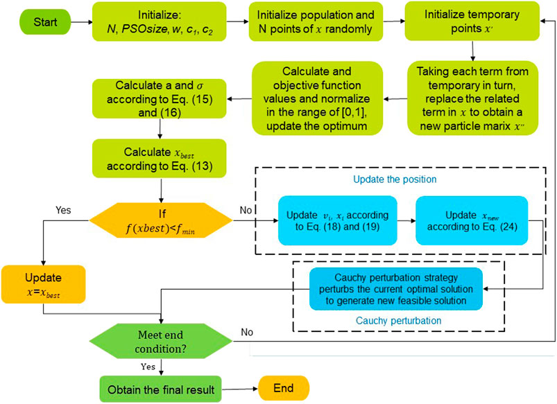
FIGURE 1. Flowchart representing the steps of HKSOPSO-CP.

4 Experimental results

The effectiveness of the HKSOPSO-CP algorithm is verified by the CEC standard test system and EED problem with four test cases with and without valve points (Zou et al., 2017).

We conducted all tests under fair comparison conditions (Zheng et al., 2021a; Zheng et al., 2022a; Zheng et al., 2022b). A potentially helpful factor in this respect is that all variables in the computing system exert a uniform effect on the performance of the compared algorithms, as per other AI-based work (Zheng et al., 2021b; Zheng et al., 2021c). The performance of HKSOPSO-CP is compared with the original KSO, PSO, and other recent algorithms. All algorithms were implemented in Matlab 2020b and ran on an Intel Core CPU aTctMTA3MDBANC41OUdIeg== (8 CPU), 32 GB RAM system.

4.1 Comparison on CEC benchmark functions

In this section, the proposed HKSOPSO-CP algorithm is compared with the original KSO, PSO, and other algorithms proposed in recent years, such as SOA (Dhiman and Kumar, 2018), TSA (Kaur et al., 2020), SSA (Xue and Shen, 2020), RSA (Abualigah et al., 2021), BWOA (Hayyolalam and Pourhaji Kazem, 2019), and COCA (Pierezan and Coelho, 2018). Tables 1–3 give the 23 CEC benchmark functions used in the experimental study, including unimodal test functions, multimodal test functions, and multimodal test functions with fixed dimensionality.

TABLE 1

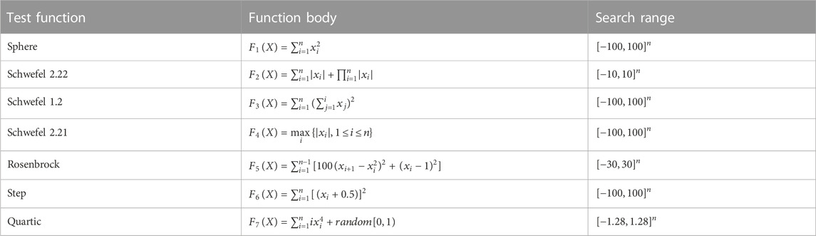
TABLE 1. Unimodal test functions.

TABLE 2

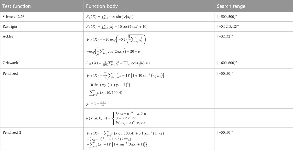
TABLE 2. Multimodal test functions.

TABLE 3

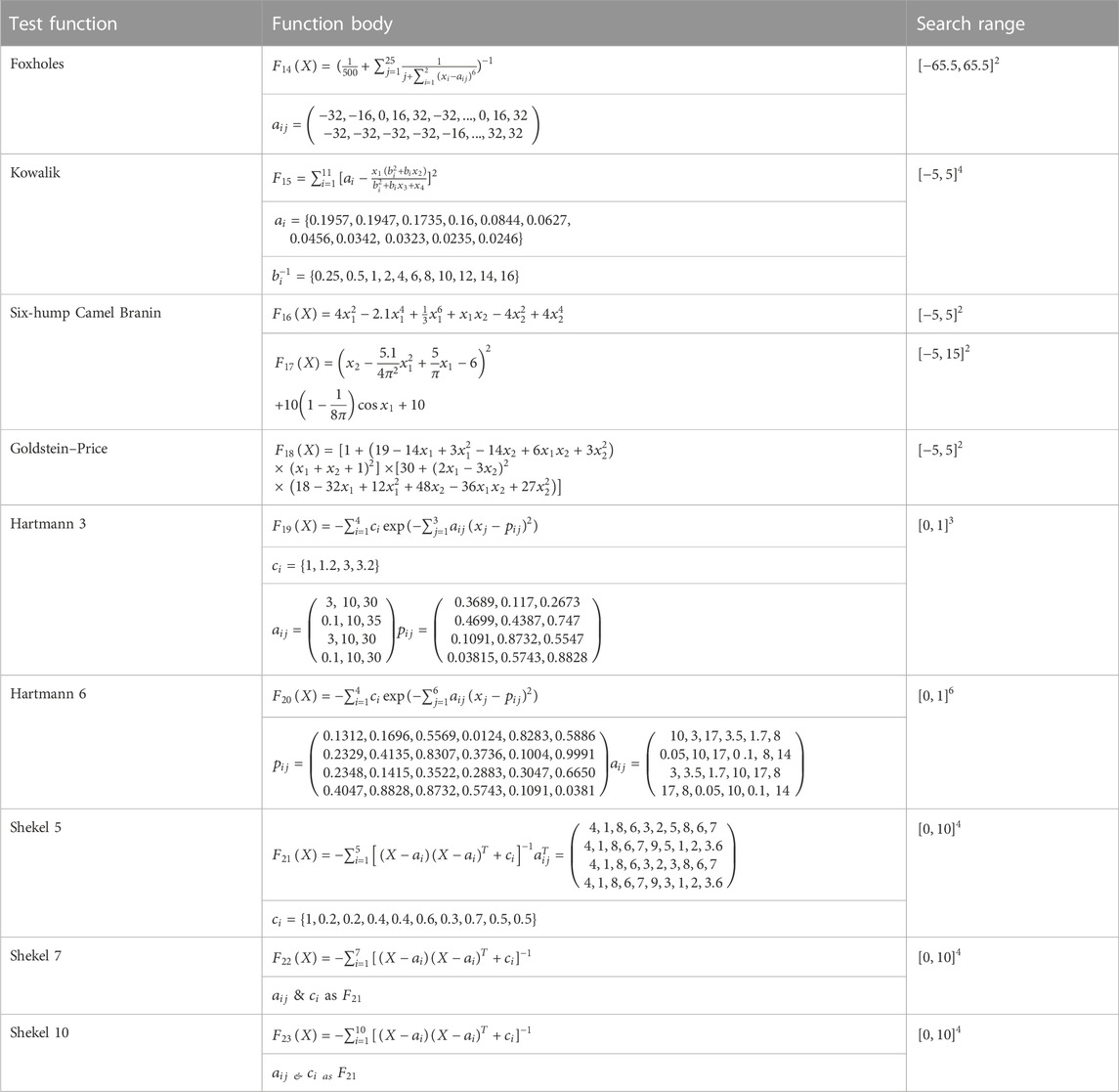
TABLE 3. Multimodal test functions with fixed dimensionality.

Table 4 illustrates the experimental results, including the worst, average, and best results over 30 runs. It can be seen that HKSOPSO-CP achieved the best results in most of the tests. In terms of the best result, HKSOPSO-CP obtained better results with 19 of the test functions, followed by KSO and COCA. In terms of the average result, HKSOPSO-CP again achieved the best results with 19 of the test functions, followed by COCA and KSO. Its advantages are especially apparent in dealing with multimodal test functions. The results show that HKSOPSO-CP may be capable of outperforming the algorithms included in the comparison carried out here. Therefore, HKSOPSO-CP is an effective method for handling various complex problems that require a strong search ability.

TABLE 4

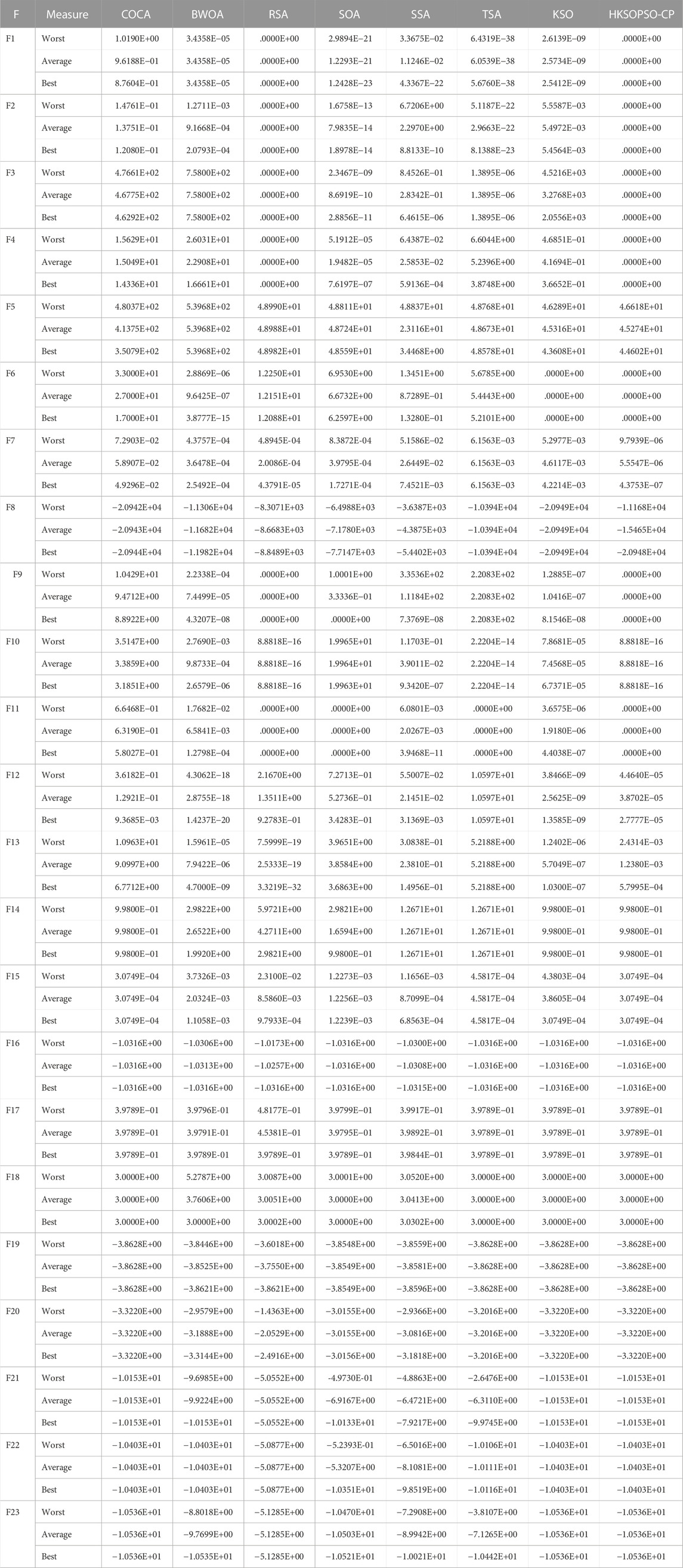
TABLE 4. The results of the comparison between methods with 23 CEC benchmark functions.

Figure 2 shows the iteration curves of HKSOPSO-CP and other algorithms participating in the comparison. In most cases, HKSOPSO-CP exhibits a strong, fast convergence ability, with a greater capacity to jump out of local optima, and its convergence effect is stabler than that of other methods. Therefore, HKSOPSO-CP offers a strong global search capability.

FIGURE 2

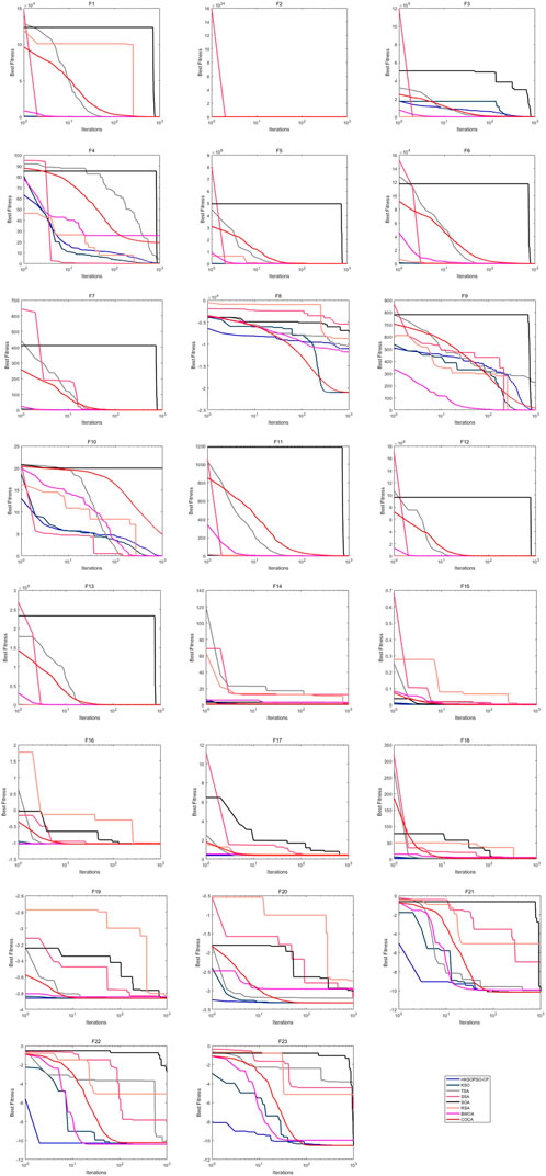
FIGURE 2. The convergence behavior of the compared methods with 23 CEC functions.

Another measure of algorithm performance is CPU running time. Figure 3 shows the CPU running time consumed by the various algorithms entered into the comparison. It can be seen that across all 23 of the test functions, the amount of time consumed by HKSOPSO-CP is relatively small, and this method is associated with the shortest running time in the case of 14 tests, performing notably better than BWOA in particular. Consequently, HKSOPSO-CP can be judged to provide better performance than KSO and other algorithms, as well as offering an improved degree of stability.

FIGURE 3

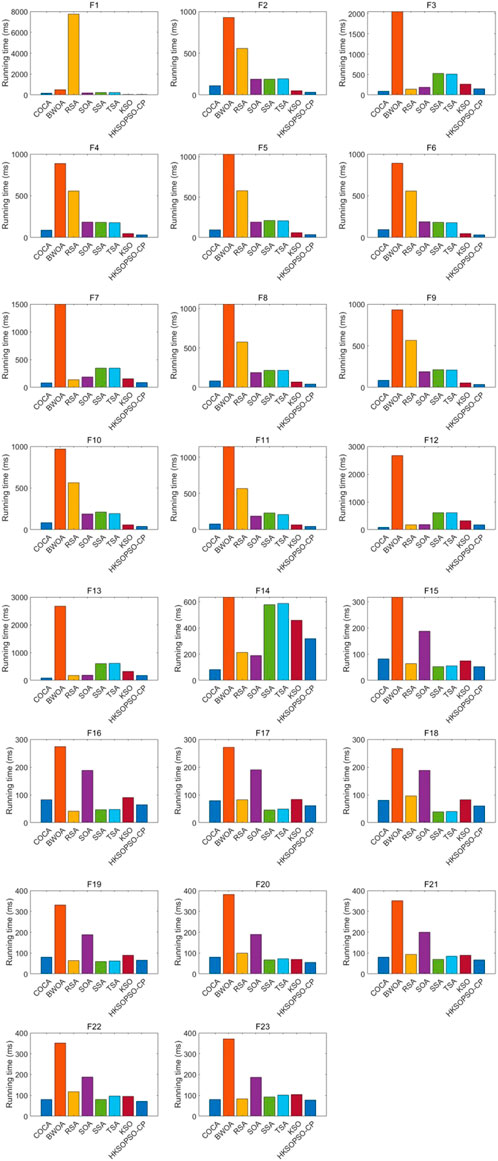
FIGURE 3. CPU running time consumed by the various algorithms entered into comparison.

4.2 Comparison of performance on the EED problem

The four test cases for the EED problem are: 1) a 6-unit system ($P_D=2.834pu)$; 2) a 10-unit system (${\mathrm{P}}_{\mathrm{D}}=2000$ MW); 3) a 40-unit system (${\mathrm{P}}_{\mathrm{D}}=10500$ MW); and 4) a 110-unit system (${\mathrm{P}}_{\mathrm{D}}=15000$ MW).

4.2.1 Case 1 comparison

In case 1, an optimization algorithm such as HKSOPSO-CP is applied to a 6-unit system with a load demand of 2.834 $\mathrm{p}\mathrm{u}$, along with other optimization algorithms handling six generators, considering the valve point effect.

Table 5 displays the results of the best solution for case 1 with a range of values for weight factor w between 0 and 1 and a step size of .1. The constraints are the generating constraint V and the transmission losses constraint $P_l$. As shown in this table, when the only objective function is to minimize fuel costs, HKSOPSO-CP achieves an optimal value of 605.8791($/h). When only emissions are minimized, HKSOPSO-CP achieves an optimal value of .194178 (ton/h).

TABLE 5

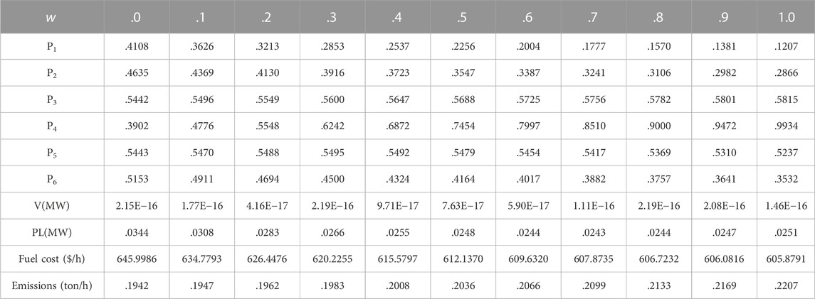
TABLE 5. Best solution values for a six-unit system with different weights.

In case 1, the HKSOPSO-CP algorithm is applied to obtain the common optimal values of fuel cost C and pollution emissions E. Figure 4 depicts the Pareto optimal values and also plots the optimal solutions provided by other algorithms. Taking the graphs and tables together, it is clear that HKSOPSO-CP achieves a better cost and overall a better compromise solution compared to NPGA (Horn et al., 1994), MOPSO (Hazra and Sinha, 2011), and NSGA (Qu et al., 2016). Other algorithms, namely MOEA/D (Abido, 2009), SPEA (Basu and Basu, 2011), MBFA (Hota et al., 2010), FSBF (Panigrahi et al., 2010), and NGPSO (Zou et al., 2017), also successfully implemented a cost-matching and compromise solution.

FIGURE 4

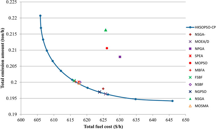
FIGURE 4. Case 1: Solutions generated by the HKSOPSO-CP algorithm, and the best compromise solutions provided by other algorithms.

Table 6 presents the results of metaheuristic algorithms in terms of minimization of costs and emissions in case 1. In the case of cost minimization, HKSOPSO-CP and SOA (Dhiman and Kumar, 2018) achieve the same optimal result of 605.8791 ($/h), which outperforms all the other algorithms, particularly MOEA/D (Abido, 2009), SPEA (Basu and Basu, 2011), MBFA (Hota et al., 2010), FSBF (Panigrahi et al., 2010), and NGPSO (Zou et al., 2017), which all achieve comparable compromise solutions. Compared with the second-best result, namely that of KSO, HKSOPSO-CP reduces fuel costs by .017 ($/h). In the case of minimization of emissions, HKSOPSO-CP achieves the optimal result among all the algorithms. These results show that HKSOPSO-CP produces a solution equivalent to or better solution than that provided by existing technology. Therefore, the HKSOPSO-CP algorithm can be considered to exhibit excellent performance in solving low-dimensionality problems.

TABLE 6

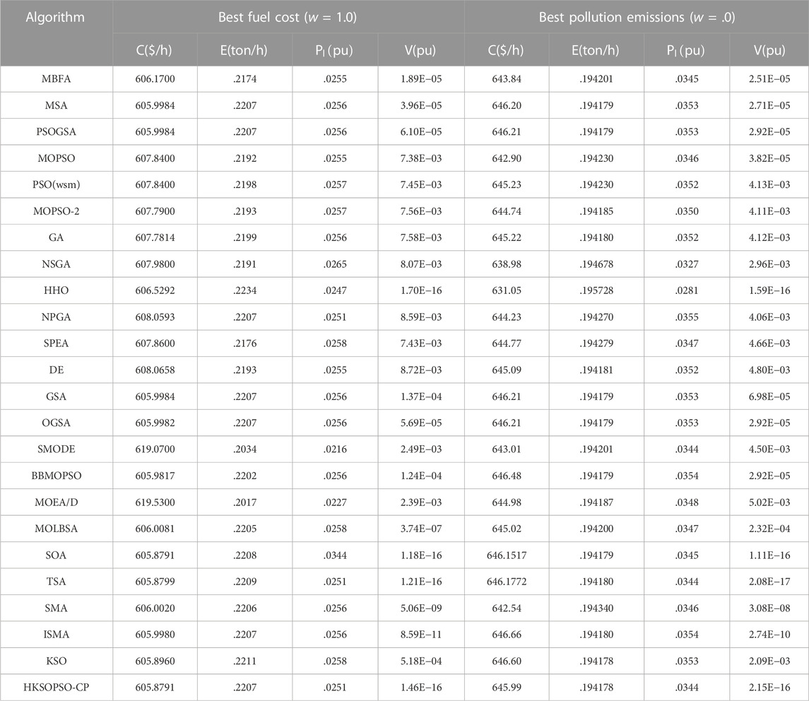
TABLE 6. Case 1 comparison between different algorithms optimizing for fuel cost or emission rate.

4.2.2 Case 2 comparison

In case 2, an optimization algorithm such as HKSOPSO-CP is applied in the same way to a ten-unit system with a load demand of 2,000 MW, and its results are compared to those of other optimization algorithms handling ten generators, considering the valve point effect.

Table 7 displays the results of the best solution for case 2 with a range of values for weight factor w between 0 and 1 and a step size of .1. As shown in this table, when the only objective function is to minimize fuel costs, HKSOPSO-CP achieves an optimal value of 11,497 ($/h). When only emissions are minimized, HKSOPSO-CP achieves an optimal value of 3,932 (ton/h).

TABLE 7

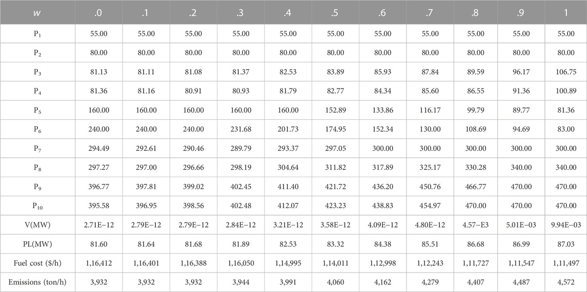
TABLE 7. Best solution values for a 10-unit system with different weights.

In case 2, the HKSOPSO-CP algorithm is applied to obtain the common optimal values of fuel cost C and pollution emissions E. Figure 5 depicts the Pareto optimal values and also plots the optimal solutions provided by other algorithms. Taking the graphs and tables together, it is clear that HKSOPSO-CP achieves a better cost and overall a better compromise solution compared to FPA (Abdelaziz et al., 2016b), NSGA (Qu et al., 2016), and SPEA2 (Basu and Basu, 2011). Other algorithms, namely BSA (Modiri-Delshad and Abd Rahim, 2015), OGHS (Singh and Dhillon, 2016), NGPSO (Zou et al., 2017), SMA (Hassan et al., 2021), and ISMA (Hassan et al., 2021), also successfully implemented a cost-matching and compromise solution.

FIGURE 5

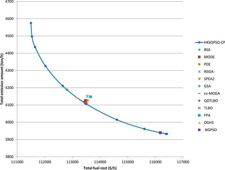
FIGURE 5. Case 2: solutions generated by the HKSOPSO-CP algorithm, and the best compromise solutions provided by other algorithms.

Table 8 and Table 9 present the results of metaheuristic algorithms in terms of minimization of costs and emissions in case 2. In the case of cost minimization, HKSOPSO-CP achieves the best optimal result of 111496.97 ($/h) compared with other algorithms, particularly SOA (Dhiman and Kumar, 2018), TSA (Kaur et al., 2020), OGHS (Singh and Dhillon, 2016), SMA (Hassan et al., 2021), and ISMA (Hassan et al., 2021), which all achieve comparable compromise solutions. Compared with the second-best result, namely that of KSO, HKSOPSO-CP reduces fuel costs by .3 ($/h). In the case of minimization of emissions, HKSOPSO-CP achieves the optimal result among all the algorithms. This shows that HKSOPSO-CP generates comparable or better quality solutions as compared to existing techniques in case 2.

TABLE 8

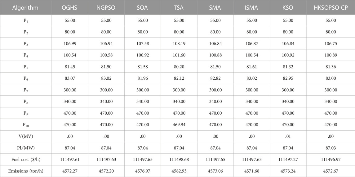
TABLE 8. Case 2 comparison between different algorithms optimizing for fuel cost.

TABLE 9

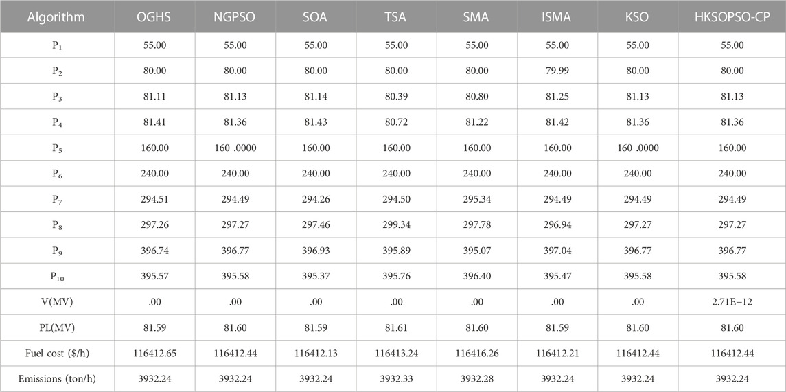
TABLE 9. Case 2 comparison between different algorithms optimizing for emission rate.

4.2.3 Case 3 comparison

A better illustration of the effectiveness of the HKSOPSO-CP algorithm is to implement it for case 3. Case 3 can be used to study the applicability of the proposed methods in the case of a 40-unit system with a load demand of 10,500 MW.

Table 10 displays the results of the best solution for case 3 with a range of values for weight factor w between 0 and 1 and a step size of .1. As shown in this table, when the only objective function is to minimize fuel costs, HKSOPSO-CP achieves an optimal value of 176682 (ton/h). When only emissions are minimized, HKSOPSO-CP achieves an optimal value of 121374($/h).

TABLE 10

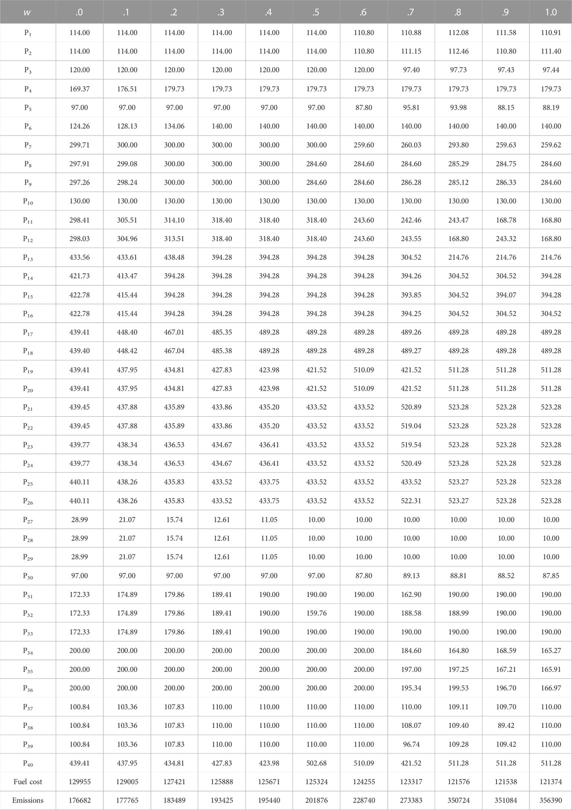
TABLE 10. Best solution values for a 40-unit system with different weights.

In case 3, the HKSOPSO-CP algorithm is applied to obtain the common optimal values of fuel cost C and pollution emissions E. Figure 6 depicts the Pareto optimal values and also plots the optimal solutions provided by other algorithms. Taking the graphs and tables together, it is clear that HKSOPSO-CP achieves a better cost and overall a better compromise solution compared to NSGA (Modiri-Delshad and Abd Rahim, 2015), GSA (Özyön et al., 2015), and NSPSO (Zou et al., 2017). Other algorithms, namely QOTLBO (Roy and Bhui, 2013), LMPSO (Jadoun et al., 2015), SMA (Hassan et al., 2021), and ISMA (Hassan et al., 2021), also successfully implemented a cost-matching and compromise solution.

FIGURE 6

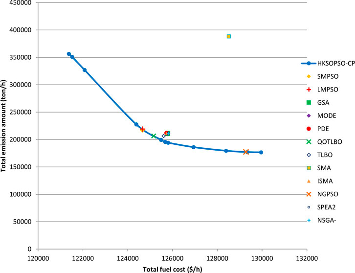
FIGURE 6. Case 3: Solutions generated by the HKSOPSO-CP algorithm, and the best compromise solutions provided by other algorithms.

Table 11 presents the results of metaheuristic algorithms in terms of minimization of costs and emissions in case 3. In the case of cost minimization, HKSOPSO-CP achieves the best optimal result of 1,21,374 ($/h) in comparison to all the other algorithms, particularly LMPSO (Jadoun et al., 2015), SOA (Dhiman and Kumar, 2018), TSA (Kaur et al., 2020), SMA (Hassan et al., 2021), and ISMA (Hassan et al., 2021), which all achieve comparable compromise solutions. Compared with the second-best result, namely that of KSO, HKSOPSO-CP reduces fuel costs by 2.0 ($/h). In the case of minimization of emissions, HKSOPSO-CP achieves the optimal result among all the algorithms. The results show that HKSOPSO-CP produces a solution that is equivalent to or better than those provided by existing technology in case 3.

TABLE 11

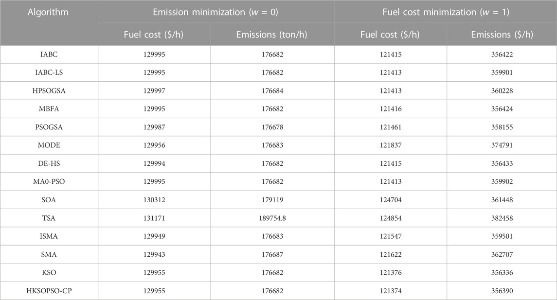
TABLE 11. Case 3 comparison between different algorithms optimizing for fuel cost or emission rate.

4.2.4 Case 4 comparison

In case 4, HKSOPSO-CP is applied, along with several other optimization algorithms for comparison, to a 110-unit system with a load demand of 15,000 MW, with a valve point effect and no transmission loss.

Table 12 presents the results of metaheuristic algorithms in terms of minimization of costs and emissions in case 4. In the case of cost minimization, HKSOPSO-CP achieves the best result of 198526.78 ($/h) when compared with all other algorithms, particularly SSA and TSA, which achieve comparable solutions on the benchmark function test. Compared with the second-best result, namely that of ISMA (Hassan et al., 2021), HKSOPSO-CP reduces fuel costs by 39.12 ($/h). These results show that HKSOPSO-CP obtains solutions that are comparable to or better than those provided by existing techniques in case 4. Therefore, the HKSOPSO-CP algorithm can be considered to provide improved performance in solving high-dimensionality EED problems.

TABLE 12

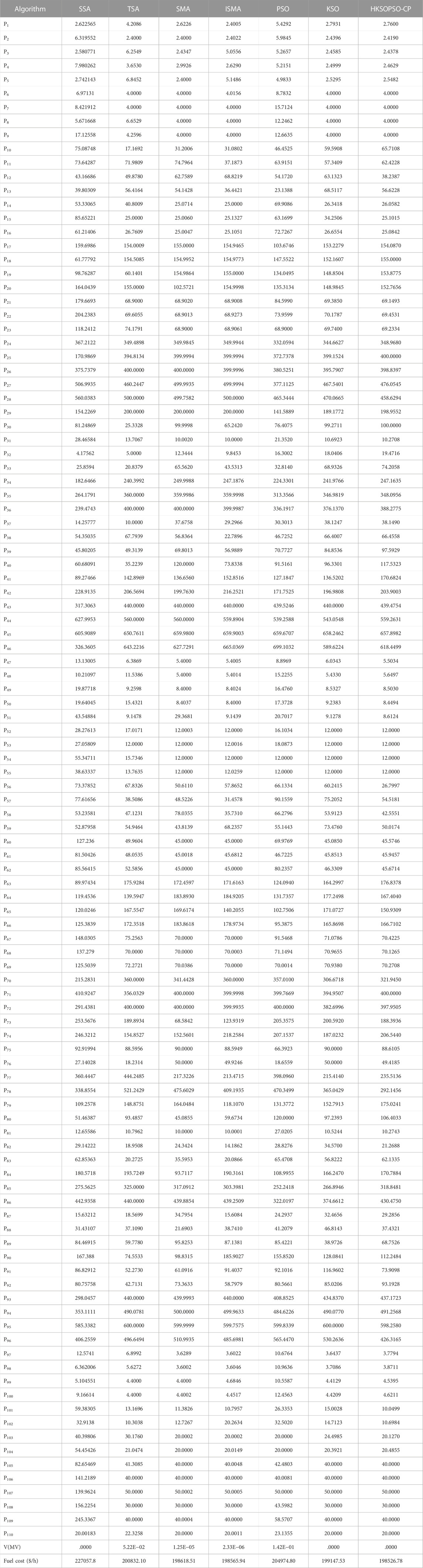
TABLE 12. Case 4 comparison between different algorithms optimizing for fuel cost.

Overall, SOA offers nearly the same performance as HKSOPSO when dealing with low-dimensionality problems, but it is less effective when dealing with high-dimensionality problems. HKSOPSO-CP provides the optimal results in solving problems of different dimensionalities, which indicates that this method offers better performance and versatility than other algorithms; for this reason, it can be applied to more fields, such as hybrid motion models (Wu et al., 2022), structured sparsity optimization (Zhang et al., 2022b), recommender systems (Li et al., 2014; Li et al., 2017), image-to-image translation (Zhang et al., 2022c), human activity recognition (Qiu et al., 2022), dynamic module detection (Li et al., 2021), location-based services (Wu et al., 2020b; Wu et al., 2021b), smart contract vulnerability detection (Zhang et al., 2022d), power flow optimization (Cao et al., 2022b), image denoising (Zhang et al., 2020), and medical data processing (Guo et al., 2022).

5 Conclusion

A novel hybrid approach, in the form of the HKSOPSO-CP optimization algorithm, is presented in this paper and is successfully applied to solve the EED problem in power systems, accounting for the valve point effect. The HKSOPSO-CP method is applied in four real-world cases, involving 6, 10, 40, and 110 generating units with various power system constraints. It has been demonstrated that the proposed algorithm is capable of providing better solutions than conventional KSO and other algorithms used as points of comparison. The results also show that the proposed algorithm is robust and flexible. In the future, this method can be used to solve other complex optimization problems. Moreover, different kernel functions could be used to solve some optimization problems to achieve better results; however, to enable this, it will be necessary to focus on computational tricks for kernel mapping. Meanwhile, research will focus on applying the HKSOPSO-CP approach and its variants to other real-world problems, such as medical data classification and complex multi-objective problems in engineering.

Data availability statement

The original contributions presented in the study are included in the article/Supplementary Material, further inquiries can be directed to the corresponding authors.

Author contributions

RD: Writing—original draft, writing—review and editing, software, visualization, investigation. LM: Writing—Original draft, writing—Review and editing, software, visualization, investigation. HC: Conceptualization, methodology, formal analysis, investigation, writing—Review and editing, funding acquisition, supervision. AH: Writing—original draft, writing—review and editing, software, visualization, investigation. GL: Conceptualization, methodology, formal analysis, investigation, writing—review and editing, funding acquisition, supervision.

Funding

This research was supported by the Science and Technology Development Project of Jilin Province, China (YDZJ202201ZYTS555), the Science and Technology Research Project of the Education Department of Jilin Province, China (JJKH20220244KJ), and the Zhejiang Provincial Philosophy and Social Sciences Planning Project (23NDJC393YBM).

Conflict of interest

The authors declare that the research was conducted in the absence of any commercial or financial relationships that could be construed as a potential conflict of interest.

Publisher’s note

All claims expressed in this article are solely those of the authors and do not necessarily represent those of their affiliated organizations, or those of the publisher, the editors and the reviewers. Any product that may be evaluated in this article, or claim that may be made by its manufacturer, is not guaranteed or endorsed by the publisher.

References

Abdelaziz, A., Ali, E., and Abd-Elazim, S. (2016). Combined economic and emission dispatch solution using flower pollination algorithm. Int. J. Electr. Power Energy Syst. 80, 264–274. doi:10.1016/j.ijepes.2015.11.093

CrossRef Full Text | Google Scholar

Abdelaziz, A., Ali, E., and Abd-Elazim, S. (2016). Implementation of flower pollination algorithm for solving economic load dispatch and combined economic emission dispatch problems in power systems. Energy 101, 506–518. doi:10.1016/j.energy.2016.02.041

CrossRef Full Text | Google Scholar

Abido, M. A. (2009). “Multiobjective evolutionary algorithms for electric power dispatch problem,” in Computational intelligence (Springer), 47–82.

CrossRef Full Text | Google Scholar

Abualigah, L., Elaziz, M. A., Sumari, P., Geem, Z. W., and Gandomi, A. H. (2021). Reptile search algorithm (RSA): A nature-inspired meta-heuristic optimizer. Expert Syst. Appl. 191, 116158. doi:10.1016/j.eswa.2021.116158

CrossRef Full Text | Google Scholar

Ahmadianfar, I., Heidari, A. A., Gandomi, A. H., Chu, X., and Chen, H. (2021). RUN beyond the metaphor: An efficient optimization algorithm based on Runge Kutta method. Expert Syst. Appl. 181, 115079. doi:10.1016/j.eswa.2021.115079

CrossRef Full Text | Google Scholar

Ahmadianfar, I., Heidari, A. A., Noshadian, S., Chen, H., and Gandomi, A. H. (2022). INFO: An efficient optimization algorithm based on weighted mean of vectors. Expert Syst. Appl. 195, 116516. doi:10.1016/j.eswa.2022.116516

CrossRef Full Text | Google Scholar

Basu, M., and Basu, M. (2011). Economic environmental dispatch using multi-objective differential evolution. Appl. Soft Comput. 11 (2), 28452845–28532853. doi:10.1016/j.asoc.2010.11.014

CrossRef Full Text | Google Scholar

Cao, B., Gu, Y., Lv, Z., Yang, S., Zhao, J., and Li, Y. (2020). RFID reader anticollision based on distributed parallel particle swarm optimization. IEEE Internet Things J. 8 (5), 3099–3107. doi:10.1109/jiot.2020.3033473

CrossRef Full Text | Google Scholar

Cao, B., Yan, Y., Wang, Y., Liu, X., Lin, J. C. W., Sangaiah, A. K., et al. (2022). A multiobjective intelligent decision-making method for multistage placement of PMU in power grid enterprises. IEEE Trans. Industrial Inf., 1–9. doi:10.1109/tii.2022.3215787

CrossRef Full Text | Google Scholar

Cao, X., Wang, J., and Zeng, B. (2022). A study on the strong duality of second-order conic relaxation of AC optimal power flow in radial networks. IEEE Trans. Power Syst. 37 (1), 443–455. doi:10.1109/tpwrs.2021.3087639

CrossRef Full Text | Google Scholar

Chen, H.-L., Wang, G., Cai, Z. N., Liu, W. B., and Wang, S. J. (2016). An efficient hybrid kernel extreme learning machine approach for early diagnosis of Parkinson׳s disease. Neurocomputing 184, 131–144. doi:10.1016/j.neucom.2015.07.138

CrossRef Full Text | Google Scholar

Chen, Y. (2022). Research on collaborative innovation of key common technologies in new energy vehicle industry based on digital twin technology. Energy Rep. 8, 15399–15407. doi:10.1016/j.egyr.2022.11.120

CrossRef Full Text | Google Scholar

Cima, J. A., Matheson, A. L., and Ross, W. T. (2006). The Cauchy transform. American Mathematical Soc.

Google Scholar

de Athayde Costa e Silva, M., Klein, C. E., Mariani, V. C., and dos Santos Coelho, L. (2013). Multiobjective scatter search approach with new combination scheme applied to solve environmental/economic dispatch problem. Energy 53, 14–21. doi:10.1016/j.energy.2013.02.045

CrossRef Full Text | Google Scholar

Deng, W., Ni, H., Liu, Y., Chen, H., and Zhao, H. (2022). An adaptive differential evolution algorithm based on belief space and generalized opposition-based learning for resource allocation. Appl. Soft Comput. 127, 109419. doi:10.1016/j.asoc.2022.109419

CrossRef Full Text | Google Scholar

Deng, W., Xu, J., Gao, X. Z., and Zhao, H. (2022). An enhanced MSIQDE algorithm with novel multiple strategies for global optimization problems. IEEE Trans. Syst. Man, Cybern. Syst. 52 (3), 1578–1587. doi:10.1109/tsmc.2020.3030792

CrossRef Full Text | Google Scholar

Deng, W., Xu, J., Zhao, H., and Song, Y. (2020). A novel gate resource allocation method using improved PSO-based QEA. IEEE Trans. Intelligent Transp. Syst. 23, 1737–1745. doi:10.1109/TITS.2020.3025796

CrossRef Full Text | Google Scholar

Deng, W., Zhang, L., Zhou, X., Zhou, Y., Sun, Y., Zhu, W., et al. (2022). Multi-strategy particle swarm and ant colony hybrid optimization for airport taxiway planning problem. Inf. Sci. 612, 576–593. doi:10.1016/j.ins.2022.08.115

CrossRef Full Text | Google Scholar

Deng, W., Zhang, X., Zhou, Y., Liu, Y., Zhou, X., Chen, H., et al. (2022). An enhanced fast non-dominated solution sorting genetic algorithm for multi-objective problems. Inf. Sci. 585, 441–453. doi:10.1016/j.ins.2021.11.052

CrossRef Full Text | Google Scholar

Dhiman, G., and Kumar, V. (2018). Seagull optimization algorithm: Theory and its applications for large-scale industrial engineering problems. Knowledge-Based Syst. 165, 169–196. doi:10.1016/j.knosys.2018.11.024

CrossRef Full Text | Google Scholar

Dong, R., Chen, H., Heidari, A. A., Turabieh, H., Mafarja, M., and Wang, S. (2021). Boosted kernel search: Framework, analysis and case studies on the economic emission dispatch problem. Knowledge-Based Syst. 233, 107529. doi:10.1016/j.knosys.2021.107529

CrossRef Full Text | Google Scholar

Dong, R., and Wang, S. (2020). New optimization algorithm inspired by kernel tricks for the economic emission dispatch problem with valve point. IEEE Access 8, 16584–16594. doi:10.1109/access.2020.2965725

CrossRef Full Text | Google Scholar

El-Keib, A. A., and Ding, H. (1994). Environmentally constrained economic dispatch using linear programming. Electr. Power Syst. Res. - ELEC POWER SYST RES 29, 155–159. doi:10.1016/0378-7796(94)90010-8

CrossRef Full Text | Google Scholar

Gao, D., Wang, G.-G., and Pedrycz, W. (2020). Solving fuzzy job-shop scheduling problem using DE algorithm improved by a selection mechanism. IEEE Trans. Fuzzy Syst. 28 (12), 3265–3275. doi:10.1109/tfuzz.2020.3003506

CrossRef Full Text | Google Scholar

Ge, L., Du, T., Li, Y., Yan, J., and Rafiq, M. U. (2022). Virtual collection for distributed photovoltaic data: Challenges, methodologies, and applications. Energies 15 (23), 8783. doi:10.3390/en15238783

CrossRef Full Text | Google Scholar

Ge, L., Li, Y., Li, Y., Yan, J., and Sun, Y. (2022). Smart distribution network situation awareness for high-quality operation and maintenance: A brief Review. Energies 15 (3), 828. doi:10.3390/en15030828

CrossRef Full Text | Google Scholar

Goudarzi, A., Li, Y., and Xiang, J. (2019). A hybrid non-linear time-varying double-weighted particle swarm optimization for solving non-convex combined environmental economic dispatch problem. Appl. Soft Comput. 86, 105894. doi:10.1016/j.asoc.2019.105894

CrossRef Full Text | Google Scholar

Guo, K., Chen, T., Ren, S., Li, N., Hu, M., and Kang, J. (2022). Federated learning empowered real-time medical data processing method for smart healthcare. IEEE/ACM Trans. Comput. Biol. Bioinforma., 1–12. doi:10.1109/tcbb.2022.3185395

CrossRef Full Text | Google Scholar

Han, X., Han, Y., Chen, Q., Li, J., Sang, H., Liu, Y., et al. (2021). Distributed flow shop scheduling with sequence-dependent setup times using an improved iterated greedy algorithm. Complex Syst. Model. Simul. 1 (3), 198–217. doi:10.23919/csms.2021.0018

CrossRef Full Text | Google Scholar

Hassan, M. H., Kamel, S., Abualigah, L., and Eid, A. (2021). Development and application of slime mould algorithm for optimal economic emission dispatch. Expert Syst. Appl. 182, 115205. doi:10.1016/j.eswa.2021.115205

CrossRef Full Text | Google Scholar

Hayyolalam, V., and Pourhaji Kazem, A. A. (2019). Black widow optimization algorithm: A novel meta-heuristic approach for solving engineering optimization problems ✩. Eng. Appl. Artif. Intell. 87, 103249. doi:10.1016/j.engappai.2019.103249

CrossRef Full Text | Google Scholar

Hazra, J., and Sinha, A. (2011). A multi-objective optimal power flow using particle swarm optimization. Eur. Trans. Electr. power 21 (1), 1028–1045. doi:10.1002/etep.494

CrossRef Full Text | Google Scholar

He, Z., Yen, G. G., and Ding, J. (2020). Knee-based decision making and visualization in many-objective optimization. IEEE Trans. Evol. Comput. 25 (2), 292–306. doi:10.1109/tevc.2020.3027620

CrossRef Full Text | Google Scholar

Heidari, A. A., Mirjalili, S., Faris, H., Aljarah, I., Mafarja, M., and Chen, H. (2019). Harris hawks optimization: Algorithm and applications. Future Generation Comput. Systems-the Int. J. Escience 97, 849–872. doi:10.1016/j.future.2019.02.028

CrossRef Full Text | Google Scholar

Horn, J., Nafpliotis, N., and Goldberg, D. E. (1994). “A niched Pareto genetic algorithm for multiobjective optimization,” in Proceedings of the first IEEE conference on evolutionary computation. IEEE world congress on computational intelligence, Orlando, FL, USA, 27-29 June 1994 (IEEE).

Google Scholar

Hosny, M., Kamel, S., Abualigah, L., and Eid, A. (2021). Development and application of slime mould algorithm for optimal economic emission dispatch. Expert Syst. Appl. 182, 115205. doi:10.1016/j.eswa.2021.115205

CrossRef Full Text | Google Scholar

Hota, P., Barisal, A., and Chakrabarti, R. (2010). Economic emission load dispatch through fuzzy based bacterial foraging algorithm. Int. J. Electr. Power & Energy Syst. 32, 794–803. doi:10.1016/j.ijepes.2010.01.016

CrossRef Full Text | Google Scholar

Hu, J., Gui, W., Heidari, A. A., Cai, Z., Liang, G., Chen, H., et al. (2022). Dispersed foraging slime mould algorithm: Continuous and binary variants for global optimization and wrapper-based feature selection. Knowledge-Based Syst. 237, 107761. doi:10.1016/j.knosys.2021.107761

CrossRef Full Text | Google Scholar

Hua, Y., Liu, Q., Hao, K., and Jin, Y. (2021). A survey of evolutionary algorithms for multi-objective optimization problems with irregular Pareto fronts. IEEE/CAA J. Automatica Sinica 8 (2), 303–318. doi:10.1109/jas.2021.1003817

CrossRef Full Text | Google Scholar

Hussien, A. G., Heidari, A. A., Ye, X., Liang, G., Chen, H., and Pan, Z. (2022). Boosting whale optimization with evolution strategy and Gaussian random walks: An image segmentation method. Eng. Comput. doi:10.1007/s00366-021-01542-0

CrossRef Full Text | Google Scholar

Jadhav, H. T., Raj, S., and Roy, R. (2013). Solution to economic emission load dispatch problem using modified artificial bee colony algorithm. 1–6.

CrossRef Full Text | Google Scholar

Jadoun, V. K., Gupta, N., Niazi, K. R., and Swarnkar, A. (2015). Modulated particle swarm optimization for economic emission dispatch. Int. J. Electr. Power & Energy Syst. 73, 80–88. doi:10.1016/j.ijepes.2015.04.004

CrossRef Full Text | Google Scholar

Kaur, S., Dhiman, G., and Sangal, A. (2020). Tunicate swarm algorithm: A new bio-inspired based metaheuristic paradigm for global optimization. Eng. Appl. Artif. Intell. 90, 103541. doi:10.1016/j.engappai.2020.103541

CrossRef Full Text | Google Scholar

Kennedy, J., and Eberhart, R. (1995). “Particle swarm optimization,” in Proceedings of ICNN'95-international conference on neural networks (IEEE).

Google Scholar

Kumar, R., Sadu, A., and Panda, S. (2012). A novel multiobjective directed bee colony optimization algorithm for multiobjective emission constrained economic power dispatch. Int. J. Electr. Power & Energy Syst. 43, 1241–1250. doi:10.1016/j.ijepes.2012.06.011

CrossRef Full Text | Google Scholar

Li, D., Zhang, S., and Ma, X. (2021). Dynamic module detection in temporal attributed networks of cancers. IEEE/ACM Trans. Comput. Biol. Bioinforma. 19, 2219–2230. doi:10.1109/TCBB.2021.3069441

CrossRef Full Text | Google Scholar

Li, J.-Y., Zhan, Z. H., Wang, C., Jin, H., and Zhang, J. (2020). Boosting data-driven evolutionary algorithm with localized data generation. IEEE Trans. Evol. Comput. 24 (5), 923–937. doi:10.1109/tevc.2020.2979740

CrossRef Full Text | Google Scholar

Li, J., Chen, C., Chen, H., and Tong, C. (2017). Towards context-aware social recommendation via individual trust. Knowledge-Based Syst. 127, 58–66. doi:10.1016/j.knosys.2017.02.032

CrossRef Full Text | Google Scholar

Li, J., Zheng, X. L., Chen, S. T., Song, W. W., and Chen, D. r. (2014). An efficient and reliable approach for quality-of-service-aware service composition. Inf. Sci. 269, 238–254. doi:10.1016/j.ins.2013.12.015

CrossRef Full Text | Google Scholar

Li, S., Chen, H., Wang, M., Heidari, A. A., and Mirjalili, S. (2020). Slime mould algorithm: A new method for stochastic optimization. Future Gener. Comput. Syst. 111, 300–323. doi:10.1016/j.future.2020.03.055

CrossRef Full Text | Google Scholar

Lin, Y., Song, H., Ke, F., Yan, W., Liu, Z., and Cai, F. (2022). Optimal caching scheme in D2D networks with multiple robot helpers. Comput. Commun. 181, 132–142. doi:10.1016/j.comcom.2021.09.027

CrossRef Full Text | Google Scholar

Liu, Y., Heidari, A. A., Cai, Z., Liang, G., Chen, H., Pan, Z., et al. (2022). Simulated annealing-based dynamic step shuffled frog leaping algorithm: Optimal performance design and feature selection. Neurocomputing 503, 325–362. doi:10.1016/j.neucom.2022.06.075

CrossRef Full Text | Google Scholar

Mavrovouniotis, M., and Yang, S. (2011). A memetic ant colony optimization algorithm for the dynamic travelling salesman problem. Soft Comput. 15, 1405–1425. doi:10.1007/s00500-010-0680-1

CrossRef Full Text | Google Scholar

Modiri-Delshad, M., and Abd Rahim, N. (2015). Multi-objective backtracking search algorithm for economic emission dispatch problem. Appl. Soft Comput. 40.

Google Scholar

Özyön, S., Yasar, C., Durmus, B., and Temurtas, H. (2015). Opposition-based gravitational search algorithm applied to economic power dispatch problems consisting of thermal units with emission constraints. Turkish J. Electr. Eng. Comput. Sci. 23, 2278–2288. doi:10.3906/elk-1305-258

CrossRef Full Text | Google Scholar

Panigrahi, B., Ravikumar Pandi, V., Das, S., and Das, S. (2010). Multiobjective fuzzy dominance based bacterial foraging algorithm to solve economic emission dispatch problem. Energy 35, 4761–4770. doi:10.1016/j.energy.2010.09.014

CrossRef Full Text | Google Scholar

Pierezan, J., and Coelho, L. (2018). Coyote optimization algorithm: A new metaheuristic for global optimization problems. 1–8.

CrossRef Full Text | Google Scholar

Qiu, S., Zhao, H., Jiang, N., Wang, Z., Liu, L., An, Y., et al. (2022). Multi-sensor information fusion based on machine learning for real applications in human activity recognition: State-of-the-art and research challenges. Inf. Fusion 80, 241–265. doi:10.1016/j.inffus.2021.11.006

CrossRef Full Text | Google Scholar

Qu, B.-Y., Liang, J., Zhu, Y., Wang, Z., and Suganthan, P. (2016). Economic emission dispatch problems with stochastic wind power using summation based multi-objective evolutionary algorithm. Inf. Sci. 351, 48–66. doi:10.1016/j.ins.2016.01.081

CrossRef Full Text | Google Scholar

Roy, P., and Bhui, S. (2013). Multi-objective quasi-oppositional teaching learning based optimization for economic emission load dispatch problem. Int. J. Electr. Power & Energy Syst. 53, 937–948. doi:10.1016/j.ijepes.2013.06.015

CrossRef Full Text | Google Scholar

Sierpina, V. (2013). Steven PrattSuperFoods rx for PregnancyRefstyled. Canada: John Wiley & Sons Limited. Canada. EXPLORE: The Journal of Science and Healing 9.

Google Scholar

Singh, M., and Dhillon, J. S. (2016). Multiobjective thermal power dispatch using opposition-based greedy heuristic search. Int. J. Electr. Power & Energy Syst. 82, 339–353. doi:10.1016/j.ijepes.2016.03.016

CrossRef Full Text | Google Scholar

Song, Y., Cai, X., Zhou, X., Zhang, B., Chen, H., Li, Y., et al. (2023). Dynamic hybrid mechanism-based differential evolution algorithm and its application. Expert Syst. Appl. 213, 118834. doi:10.1016/j.eswa.2022.118834

CrossRef Full Text | Google Scholar

Tu, J., Huiling, C., Mingjing, W., and Amir, H. G. (2021). The colony predation algorithm. J. Bionic Eng. 18 (3), 674–710. doi:10.1007/s42235-021-0050

CrossRef Full Text | Google Scholar

Wu, D., Zhao, H., Song, Y., and Xu, J. (2020). An effective improved co-evolution ant colony optimisation algorithm with multi-strategies and its application. Int. J. Bio-Inspired Comput. 16 (3), 158–170. doi:10.1504/ijbic.2020.10033314

CrossRef Full Text | Google Scholar

Wang, G.-G., Gao, D., and Pedrycz, W. (2022). Solving multi-objective fuzzy job-shop scheduling problem by a hybrid adaptive differential evolution algorithm. IEEE Trans. Industrial Inf. 18, 8519–8528. doi:10.1109/tii.2022.3165636

CrossRef Full Text | Google Scholar

Wang, M., Chen, H., Yang, B., Zhao, X., Hu, L., Cai, Z., et al. (2017). Toward an optimal kernel extreme learning machine using a chaotic moth-flame optimization strategy with applications in medical diagnoses. Neurocomputing 267, 69–84. doi:10.1016/j.neucom.2017.04.060

CrossRef Full Text | Google Scholar

Wang, Y., Wen, X., Gu, B., and Gao, F. (2022). Power scheduling optimization method of wind-hydrogen integrated energy system based on the improved AUKF algorithm. Mathematics 10 (22), 4207. doi:10.3390/math10224207

CrossRef Full Text | Google Scholar

Wu, S.-H., Zhan, Z.-H., and Zhang, J. (2021). Safe: Scale-adaptive fitness evaluation method for expensive optimization problems. IEEE Trans. Evol. Comput. 25 (3), 478–491. doi:10.1109/tevc.2021.3051608

CrossRef Full Text | Google Scholar

Wu, Y., Sheng, H., Zhang, Y., Wang, S., Xiong, Z., and Ke, W. (2022). Hybrid motion model for multiple object tracking in mobile devices. IEEE Internet Things J., 1. doi:10.1109/jiot.2022.3219627

CrossRef Full Text | Google Scholar

Wu, Z., Li, G., Shen, S., Lian, X., Chen, E., and Xu, G. (2021). Constructing dummy query sequences to protect location privacy and query privacy in location-based services. World Wide Web 24 (1), 25–49. doi:10.1007/s11280-020-00830-x

CrossRef Full Text | Google Scholar

Wu, Z., Wang, R., Li, Q., Lian, X., Xu, G., Chen, E., et al. (2020). A location privacy-preserving system based on query range cover-up or location-based services. IEEE Trans. Veh. Technol. 69, 5244–5254. doi:10.1109/tvt.2020.2981633

CrossRef Full Text | Google Scholar

Xu, Y., Chen, H., Heidari, A. A., Luo, J., Zhang, Q., Zhao, X., et al. (2019). An efficient chaotic mutative moth-flame-inspired optimizer for global optimization tasks. Expert Syst. Appl. 129, 135–155. doi:10.1016/j.eswa.2019.03.043

CrossRef Full Text | Google Scholar

Xue, J.-K., and Shen, B. (2020). A novel swarm intelligence optimization approach: Sparrow search algorithm. Syst. Sci. Control Eng. 8, 22–34. doi:10.1080/21642583.2019.1708830

CrossRef Full Text | Google Scholar

Yang, Y., Chen, H., Heidari, A. A., and Gandomi, A. H. (2021). Hunger games search: Visions, conception, implementation, deep analysis, perspectives, and towards performance shifts. Expert Syst. Appl. 177, 114864. doi:10.1016/j.eswa.2021.114864

CrossRef Full Text | Google Scholar

Yaşar, C., and Özyön, S. (2012). Solution to scalarized environmental economic power dispatch problem by using genetic algorithm. Int. J. Electr. Power & Energy Syst. 38, 54–62. doi:10.1016/j.ijepes.2011.12.020

CrossRef Full Text | Google Scholar

Yu, H., Song, J., Chen, C., Heidari, A. A., Liu, J., Chen, H., et al. (2022). Image segmentation of Leaf Spot Diseases on Maize using multi-stage Cauchy-enabled grey wolf algorithm. Eng. Appl. Artif. Intell. 109, 104653. doi:10.1016/j.engappai.2021.104653

CrossRef Full Text | Google Scholar

Zhan, J., Wu, Q. H., Guo, C. X., and Zhou, X. X. (2014). Fast $\lambda$-Iteration method for economic dispatch with prohibited operating zones. IEEE Trans.29, 990–991. doi:10.1109/tpwrs.2013.2287995

CrossRef Full Text | Google Scholar

Zhang, K., Wang, Z., Chen, G., Zhang, L., Yang, Y., Yao, C., et al. (2022). Training effective deep reinforcement learning agents for real-time life-cycle production optimization. J. Petroleum Sci. Eng. 208, 109766. doi:10.1016/j.petrol.2021.109766

CrossRef Full Text | Google Scholar

Zhang, L., Wang, J., Wang, W., Jin, Z., Su, Y., and Chen, H. (2022). Smart contract vulnerability detection combined with multi-objective detection. Comput. Netw. 217, 109289. doi:10.1016/j.comnet.2022.109289

CrossRef Full Text | Google Scholar

Zhang, X., Fan, C., Xiao, Z., Zhao, L., Chen, H., and Chang, X. (2022). Random reconstructed unpaired image-to-image translation. IEEE Trans. Industrial Inf., 1. doi:10.1109/TII.2022.3160705

CrossRef Full Text | Google Scholar

Zhang, X., Zheng, J., Wang, D., Tang, G., Zhou, Z., and Lin, Z. (2022). Structured sparsity optimization with non-convex surrogates of l_{2, 0}-norm: A unified algorithmic framework. IEEE Trans. Pattern Analysis Mach. Intell., 1–18. doi:10.1109/tpami.2022.3213716

CrossRef Full Text | Google Scholar

Zhang, X., Zheng, J., Wang, D., and Zhao, L. (2020). Exemplar-based denoising: A unified low-rank recovery framework. IEEE Trans. Circuits Syst. Video Technol. 30 (8), 2538–2549. doi:10.1109/tcsvt.2019.2927603

CrossRef Full Text | Google Scholar

Zhang, Y., Liu, R., Heidari, A. A., Wang, X., Chen, Y., Wang, M., et al. (2021). Towards augmented kernel extreme learning models for bankruptcy prediction: Algorithmic behavior and comprehensive analysis. Neurocomputing 430, 185–212. doi:10.1016/j.neucom.2020.10.038

CrossRef Full Text | Google Scholar

Zheng, W., Liu, X., Ni, X., Yin, L., and Yang, B. (2021). Improving visual reasoning through semantic representation. IEEE access 9, 91476–91486. doi:10.1109/access.2021.3074937

CrossRef Full Text | Google Scholar

Zheng, W., Liu, X., and Yin, L. (2021). Sentence representation method based on multi-layer semantic network. Appl. Sci. 11 (3), 1316. doi:10.3390/app11031316

CrossRef Full Text | Google Scholar

Zheng, W., Tian, X., Yang, B., Liu, S., Ding, Y., Tian, J., et al. (2022). A few shot classification methods based on multiscale relational networks. Appl. Sci. 12 (8), 4059. doi:10.3390/app12084059

CrossRef Full Text | Google Scholar

Zheng, W., Yin, L., Chen, X., Ma, Z., Liu, S., and Yang, B. (2021). Knowledge base graph embedding module design for Visual question answering model. Pattern Recognit. 120, 108153. doi:10.1016/j.patcog.2021.108153

CrossRef Full Text | Google Scholar

Zheng, W., Zhou, Y., Liu, S., Tian, J., Yang, B., and Yin, L. (2022). A deep fusion matching network semantic reasoning model. Appl. Sci. 12 (7), 3416. doi:10.3390/app12073416

CrossRef Full Text | Google Scholar

Zou, D., Li, S., Li, Z., and Kong, X. (2017). A new global particle swarm optimization for the economic emission dispatch with or without transmission losses. Energy Convers. Manag. 139, 45–70. doi:10.1016/j.enconman.2017.02.035

CrossRef Full Text | Google Scholar