The Economic Impact of a Renewable Biofuels/Energy Industry Supply Chain Using the Renewable Energy Economic Analysis Layers Modeling System

The University of Tennessee’s (UT) Department of Agricultural and Resource Economics models supply chains for both liquid and electricity generating technologies currently in use and/or forthcoming for the bio/renewable energy industry using the input–output model IMPLAN^®. The approach for ethanol, biodiesel, and other liquid fuels includes the establishment and production of the feedstock, transportation of the feedstock to the plant gate, and the one-time investment as well as annual operating of the facility that converts the feedstock to a biofuel. This modeling approach may also include the preprocessing and storage of feedstocks at depots. Labor/salary requirements and renewable identification number (RIN) values and credits attributable to the conversion facility, along with land-use changes for growing the feedstock are also included in the supply chain analyses. The investment and annual operating of renewable energy technologies for electricity generation for wind, solar, and digesters are modeled as well. Recent modeling emphasis has centered on the supply chain for liquid fuels using the Bureau of Economic Analysis’s 179 economic trading areas as modeling regions. These various data layers necessary to estimate the economic impact are contained in UT’s renewable energy economic analysis layers (REEAL) modeling system. This analysis provides an example scenario to demonstrate REEAL’s modeling capabilities. The conversion technology modeled is a gasification Fischer–Tropsch biorefinery with feedstock input of 495,000 metric tons per year of forest residue transported to a logging road that is less than one mile in distance. The biorefinery is expected to produce sustainable aviation fuel (SAF), diesel, and naphtha. An estimated one million tons of forest residue are required at fifty percent moisture content. Based on a technical economic assessment (TEA) developed by the Aviation Sustainability Center (ASCENT) and the quantity of hardwood residues available in the Central Appalachian region, three biorefineries could be sited each utilizing 495,000 dry metric tons per year. Each biorefinery could produce 47.5 million liters of SAF, 40.3 million liters of diesel, and 23.6 million liters of naphtha. Annual gross revenues for fuel required for the biorefineries to break even are estimated at $193.7 million per biorefinery. Break-even plant gate fuel prices when assuming RINs and 12.2 percent return on investment are $1.12 per liter for SAF, $1.15 per liter for diesel, and $0.97 per liter for naphtha. Based on IMPLAN, an input–output model, and an investment of $1.7 billion, the estimated economic annual impact to the Central Appalachian region if the three biorefineries are sited is over a half a billion dollars. Leakages occur as investment dollars leaving the region based on the regions local purchase coefficients (i.e., LPPs), which totals $500 million. This results in an estimated $2.67 billion in economic activity with a multiplier of 1.7, or for every million dollars spent, an additional $0.7 million in economic activity is generated in the regional economy. Gross regional product is estimated at $1.28 billion and employment of nearly 1,200 jobs are created during the construction period of the biorefineries, which results in $700 million in labor income with multiplier effects. Economic activity for the feedstock operations (harvesting and chipping) is estimated at slightly more than $16.8 million resulting in an additional $30 million in the economic impact. The stumpage and additional profit occurring from the harvest of the forest residues result in $40 million directly into the pockets of the resource and logging operation owners. Their subsequent expenditures resulted in a total economic activity increase of $71.4 million. These operations result in creating an estimated 103 direct jobs for a total of 195 with multiplier effects. Direct feedstock transportation expenditures of more than $36.7 million provide an estimated increase in economic activity of almost $68 million accounting for the multiplier effects.

Introduction

Economic impact analysis (EIA) is one methodology used to evaluate the impact of a policy, program, or project on the economy to a specified region. EIA is a useful analysis tool for decision-making, providing a measure of strategic goal achievement that complements the analysis of efficiency (benefit-cost) and financial feasibility. EIA provides information on the effects of events on a regional economy. Typically, the impact is measured using several indicators that include changes in business or economic activity, employment (jobs), gross regional product (GRP), and tax collections as a result of attracting a new industry to a region.

Frequently, national-, state-, and/or county-level actions are proposed to provide incentives for attracting an industry. To evaluate the potential benefits of such actions, information on changes in community welfare is sought. EIA is an important tool to assist in this decision-making providing information on not only the economic impact to input supplying industries but also the impact from the investment and annual operations of the new industry and potential job creations.

The costs of an energy policy can be determined, but the benefits generated by that policy may be difficult to estimate or very limited in what is considered. An accounting of costs is required, but the costs do not reflect how the policy will affect a state, region, or community. Not including all benefits will impact decision-making and “can prevent environmental, energy, and/or economic policy makers from capturing all the potential gains associated with pursuing energy efficiency and renewable energy policies” (Environmental Protection Agency, 2010).

Input–output analysis provides a framework for use in EIA. This method of analysis has been used since 1930s, first introduced by Wassily Leontief (Lonergan and Cocklin, 1985). Input–output (I-O) analysis, which is based on the interdependence of the different economic sectors and households that exist in a regional economy, quantifies the total economic effects of a change in the demand for a given product or service and captures relationships and interdependencies within the region of interest (Baumol, 2000). The model uses industry interdependence formed by production functions. The production functions reflect regional interdependence and are determined through transactions or purchases sectors make during production of goods and services. These relationships project change that might occur because of a demand change for inputs. Input–output modeling evaluates the initial shock of the event and its ripple effects through the economy. The event in this analysis is the creation of a “new” industry—production of sustainable aviation fuel (SAF) in Central Appalachia.

Analysis requires information on proposed transactions from the “new” industry that might occur or be lost. What that “new” industry looks like, its supply chains, what products are produced, and what impact the industry may have on existing transactions are all questions requiring information. The transactions occurring once (e.g., investment) need to be separated from the transactions occurring yearly. Some transactions will have a positive effect whereas others a negative on the region’s economy.

This information can be both expensive and quite extensive as well as proprietary to obtain. Yet, quick and accurate information is required. The University of Tennessee’s (UT) Department of Agricultural and Resource Economics has reviewed and identified supply chain information on renewable energy technologies such as electricity generation via wind, solar, geothermal, and biopower as well as biofuel generation through pyrolysis, gasification, hydro-processed esters and fatty acids (HEFAs), and other technologies. This inventory of technologies and supply chain components has been incorporated into the renewable energy economic analysis layers (REEAL) modeling system (Figure 1). While renewable technologies such as the generation of electricity via wind, solar, and digesters have been conducted in the past, recent modeling emphasis has centered on the supply chain for liquid fuels (English et al., 2006; De La Torre Ugarte, 2007; English et al., 2009a; English et al., 2009b; English et al., 2009c; English et al., 2009d; Lambert et al., 2016; Markel et al., 2019).

FIGURE 1

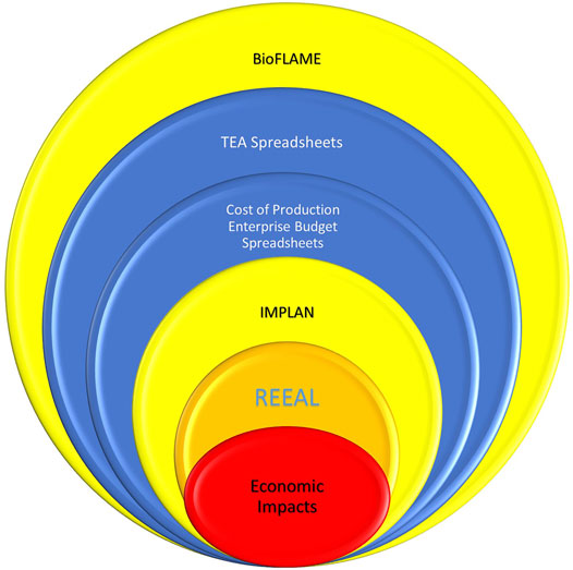
FIGURE 1. Renewable energy economic analysis layers (REEAL) modeling system and its components.

The location of these “new” industries via spatial analysis is required for decision makers. Providing regional analysis via using the Bureau of Economic Analysis’s (BEA) 179 economic trading areas provides a template for regional modeling (Figure 2). BEAs represent centers of economic activity, recognize both metropolitan and micropolitan statistical areas, and provide information on changes in economic and population growth in the United States (Johnson and Kort, 2004).

FIGURE 2

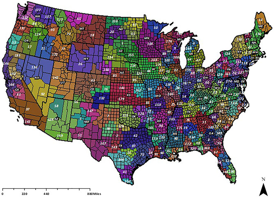
FIGURE 2. Bureau of Economic Analysis’s economic areas for input–output analysis modeling.

One existing I-O modeling system and its inherent databases for regional estimates of the economic impact occurring in a potential renewable biofuels supply chain is the IMPLAN® (IMPLAN Group LLC, 2018). The IMPLAN’s data support system provides an annual quantitative description of each U.S. county’s economic activity, which can be aggregated to multicounty economic regions. Thus, within REEAL, the economic impact is evaluated at a BEA region using multicounty-level aggregated data. From this information, regional purchase coefficients are generated to determine the leakage (purchases outside the study region) that occurs as inputs are purchased. These coefficients define where (within or outside the region) purchases are made and the proportion of goods or services used to meet intermediate or final demand that is supplied within the region of interest (Ralston, Hastings, and Brucker, 1986). Transactions occurring outside the study region (coined a “leakage” in I-O analysis) are not considered for regional economic activity. For larger events, for example, a regional model representing multiple BEAs, a larger regional or national analysis is conducted in addition to the BEA analysis. The difference in the impact between those estimated for each BEA and those estimated by the national analysis provide information on the impact of those leakages to the multiple BEA areas or the nation.

The siting or location of the technology (for example, biofuel conversion) can be specified or simulated. In this article, the location is simulated using a spatial GIS model, BioFLAME (Biofuels Facility Location Analysis Modeling Endeavor), which provides information on where the conversion technologies, feedstock, and transportation routes might be located. This spatial analytical tool is based on current infrastructure, costs, and land use (Graham, English, and Noon, 2000; He-Lambert, English, Menard, and Lambert, 2016; Sharma, Birrell, and Miguez, 2017; He-Lambert et al., 2018; Markel, English, Hellwinckel, and Menard, 2019). These models typically minimize cost of feedstock to identify potential locations. The conversion technologies modeled in REEAL provide information on what purchases are required, their infrastructure requirements, and the costs of conversion.

The supply chain in this analysis for sustainable aviation fuel and other coproduct fuels includes both downstream and upstream effects, more specifically, the establishment and production of the feedstock and the transportation of the feedstock to the plant gate and fuel from the biorefinery along with the one-time investment plus annual operating costs of the biorefinery that converts the feedstock to a biofuel. Other supply chain components may also include the preprocessing and storage of feedstocks on the “farm” or at depots. Labor/salary needs for these activities, the economic impact of renewable identification number (RIN) values and credits attributable to the conversion facility, and land-use changes for growing the feedstock are also included in this analysis. A discussion of REEAL’s components, along with an analysis example using the model, is provided.

The example provides estimates of the economic impact resulting from SAF biorefineries located in a depressed region of the United States—Central Appalachia. The feedstock available to the industry is forest residues. The technology available to convert those residues to SAF and other biofuels is based on a greenfield gasification Fischer–Tropsch technology (Brandt et al., 2021).

Methodology

Multiple information sources are used to develop REEAL. Engineering techno-economic assessment (TEA) spreadsheet tools or cost of production enterprise budgets are used to provide cost information. The TEAs represent conversion technologies for either preprocessing the feedstock or fuel conversion. The enterprise budgets provide information on feedstock and transportation. Information is also derived from the 179 I-O models developed using IMPLAN. These models incorporate the information from the spreadsheet to develop an estimate of economic impact resulting from the establishment of the technology or feedstock being investigated. The spatial land use model, BioFLAME, provides information on the extent of the impact. For each supply region that comes into solution, information on feedstock quantity, cost, miles transported, and the cost of that transportation is estimated. Adding these two cost categories provides information on break-even delivered cost to the biorefinery. Since I-O models are linear in nature, the analysis is conducted for a single conversion facility. If two or more conversion facilities locate in a particular BEA, then the economic impact increases by that factor. Table 1 indicates the current technology information available from the spreadsheets in REEAL. Also included are the general impact relating primarily to reduced expenditures because of changes in land use and increased expenditures because of changes in proprietor income and the sale of RINs.

TABLE 1

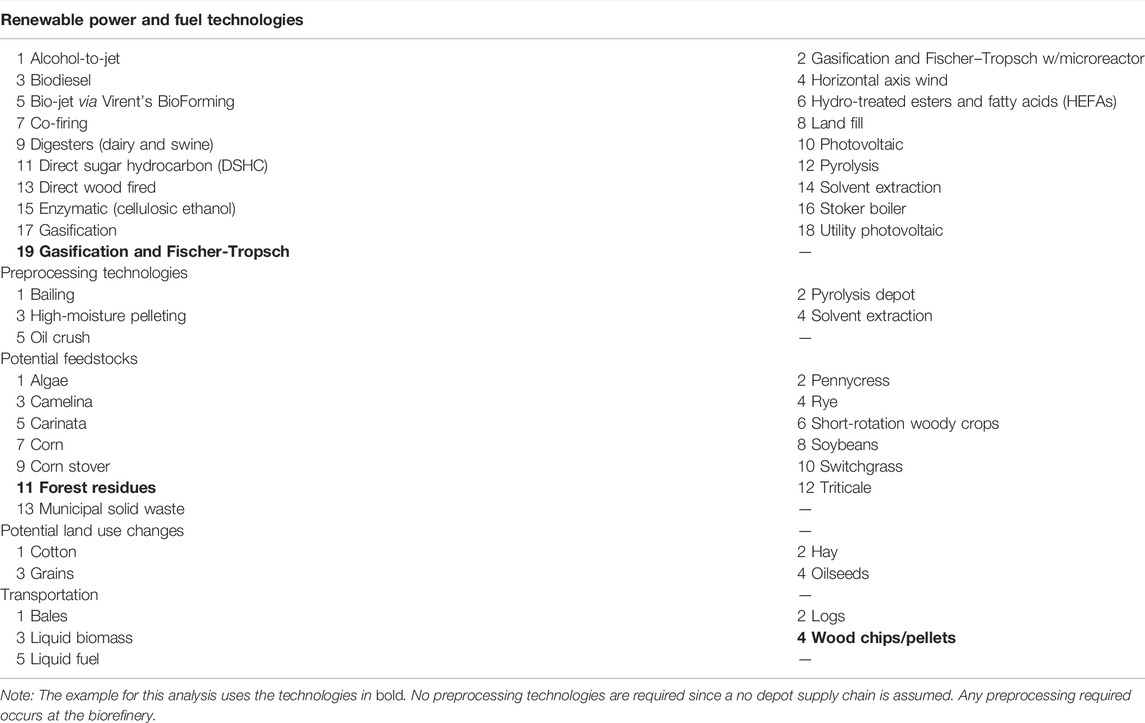
TABLE 1. Conversion and renewable energy technologies, feedstocks, and land-use changes incorporated into the renewable energy economic analysis layers modeling system.

The initial step in the development of the event is to specify the supply chain, which consists of feedstock production/maintenance/harvest, preprocessing, conversion, and distribution of products. Once defined, the scale of the preprocessing and conversion components is required, along with the type of needed feedstock—agricultural residues, forest residues, dedicated energy crops, and/or oilseeds, and the pathway, which defines the conversion technology along with some of the potential incentives that are available. In the following example, the economic impact is estimated for converting forest residues in Central Appalachia via a gasification Fischer–Tropsch (GFT) biorefinery with a feedstock input of 495,000 dry metric tons per year (1,500 metric tons per day) to demonstrate REEAL’s modeling capabilities. The supply chain consists of transporting the feedstock to a forest landing, chipping, transporting the feedstock to the biorefinery, and feedstock conversion.

Cost of Feedstock Production

Feedstock costs are derived from several sources: 1) the Billion-Ton study (U.S. Department of Energy, 2016); 2) an agricultural and forest model POLYSYS (Policy Analysis Systems Model) (English, et al., 2006; Hellwinckel, 2019); 3) ForSEAM (Forest Sustainable and Economic Analysis Model) (English et al., 2006); and 4) crop enterprise spreadsheets developed at the University of Tennessee for switchgrass, short-rotation poplar, and oilseed crops such as carinata, camelina, and pennycress. The POLYSYS database provides information on selected agricultural residues such as corn stover and wheat straw as well as additional dedicated energy crops that include Miscanthus, energy cane, and short-rotation tree species such as willow, sweetgum, and sycamore. For perennial dedicated energy herbaceous and tree crops, an establishment cost is estimated and treated as an investment in the development of the feedstock. All the crops have maintenance and harvest/collection costs. Table 2 contains information on these costs for each of the feedstocks.

TABLE 2

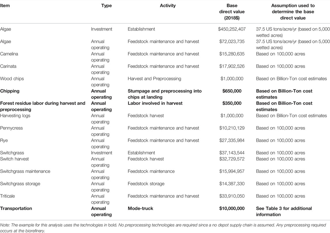
TABLE 2. Summary of the basic costs of feedstock production.

Techno-Economic Assessment Spreadsheets–Conversion and Preprocessing

ASCENT TEAs contain information on pre-specified engineering technology information on investment in the facility as well as its operation costs. The TEAs provide inputs needed, the conversion technologies output, along with information on capital expenditures (CAPEX) and operating expenditures (OPEX) (Brandt, Tanzil, Garcia-Perez, and Wolcott, 2021). Currently, ASCENT TEAs include alcohol-to-jet, gasification/Fischer–Tropsch, HEFA, gasification with microreactor, and pyrolysis. The ASCENT baseline spreadsheets calculate a break-even value for the coproducts produced assuming a 12.2 percent return on investment, and the net present value equals zero. These baseline spreadsheets have a specified throughput and feedstock that the user can change. The baseline is used to estimate the impact with an average feedstock cost. The scenarios use alternative feedstocks and capacity when compared to the baseline. This analysis uses the gasification/Fischer–Tropsch TEA in its analysis.

To meet the specification requirements of the conversion facility, preprocessing of biomass feedstock is often required. Preprocessing is either performed at the conversion facility, a depot, or in the field. Depot preprocessing spreadsheets are incorporated in REEAL for conventional and high-moisture pelleting (pellets), chipping at landing (chips), pyrolysis (oil), and crushing (oil).

BioFLAME

BioFLAME is a large-scale, multiregional optimization model that determines the least-cost locations of biofuel facilities supplying aviation fuel to airports, or other demanders, and the attendant changes in land use, given the location of the feedstock. In other words, BioFLAME determines which BEAs the biorefinery will be sited. It is currently calibrated for the southeastern US but is capable of being calibrated for other regions. BioFLAME determines the least-cost potential feedstock draw areas and possible direct land-use changes. BioFLAME operates on GIS architecture and consists of geospatial layers used to identify refinery locations (i.e., road networks and transmission lines, etc.). Information supplied includes site suitability, feedstock availability, delivered feedstock costs, transportation emissions, direct land use change, potential supply, and transportation costs. Road networks, transmission lines, and other geospatial layers are used to identify candidate refinery locations. BioFLAME provides estimates for:

• the cost-minimizing locations where feedstock would be sourced to supply a biorefinery,

• the annual cost of procuring and transporting feedstock, and

• the number of facilities a region can support.

BioFLAME has two sets of identifier nodes. The initial set is the supply regions. These regions take the form of hexagons and contain 5 square miles of area (Figure 3). The potential quantity of feedstock by type is estimated for each supply region and is assumed to be located at the centroid. The United States is divided into these hexagons, and in the Southeast, there are approximately 1.3 million supply units. Transportation is defined from the centroid of each supply region to the nearest road and then to each supply region in the model. The second set of nodes is the potential sites for conversion of the feedstock. These nodes can serve as preprocessing or conversion nodes and are known as candidate nodes. Currently, the model relies on available industrial park locations that meet the infrastructure needs of the facility being sited. In areas where this information is not known, towns with a population of 10,000 or more serve as candidate nodes. Each hexagon is assigned to a county, state, and BEA.

FIGURE 3

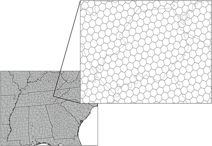
FIGURE 3. BioFLAME’s supply regions.

The solution of BioFLAME provides information on the origin of the feedstock, the destination of the feedstock, the type of feedstock, the quantity delivered, area, the costs of the feedstock (establishment, maintenance, harvesting/collection, and transportation), previous land use, and miles traveled. Ex post analysis projects change in transportation emissions and soil erosion, if cropland is involved. Embedded in BioFLAME is a transportation sector. The transportation sector contains the U.S. detailed streets TIGER 2000-based dataset enhanced by the Environmental Science Research Institute (ESRI) and Tele Atlas (ESRI, 2006). Transportation is primarily by truck originating from the farm gate or forest landing to a depot or biorefinery. In BioFLAME, the gross vehicle weight rating is a constraint on the load assumed at 36.3 MT. To arrive at a $ per MT-km cost estimate, a trip distance is assumed, along with a weight load (Table 3). In total, four different feedstock transportation types are estimated as follows: 1 forest residue and short-rotation trees in the form of chips, 2 traditional forest products in the form of logs, 3 herbaceous material in the form of bales, and 4. oil seeds and corn. In addition, a tanker truck cost carrying pyrolysis oil or final liquid fuel product is estimated. The cost estimates are based on the dry matter content of the material being trucked from field to initial destination–—depot or biorefinery. In this analysis, depots are not assumed, and feedstocks enter the biorefinery in the form of chips.

TABLE 3

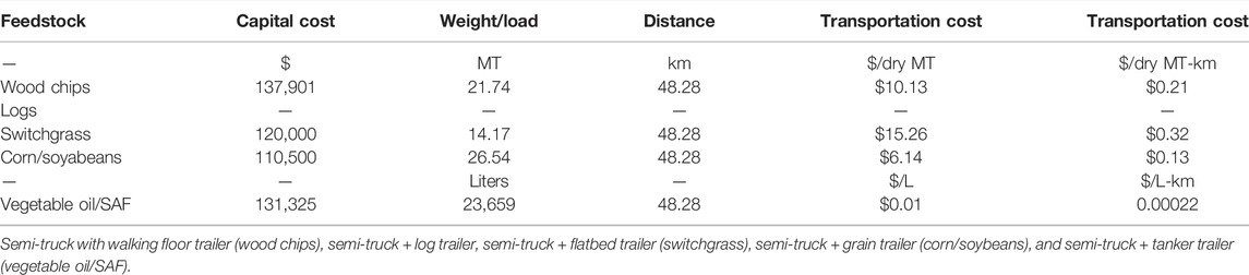
TABLE 3. Trucking cost of biomass feedstock ($/unit-km) (2017$).

Mileage is determined from the center of the supply node to each of the other supply nodes. The shortest distance and road types between supply nodes are determined and used in estimating distance and speed. Trailer types and possible payloads for those trailers are predetermined and depend on the feedstock. For instance, if bales of herbaceous feedstock are hauled with a large truck, you cannot have a 24 MT load, and the density of the feedstock will not allow it. The capacity of the trailer is 36 large round bales, 24 rectangular bales, or 13 condensed/wrapped bales. The trailer carries 13 tons in round bales, 16 tons in rectangular bales, or 26 tons in wrapped bales. A dry matter loss during transportation is two percent (Kumar and Sokhansanj, 2007; Larson et al., 2010). The quantity of green tons identified by BioFLAME in each supply region is divided by the weight per load to determine the number of trucks required to bring the material from supply node to the biorefinery or preprocessing depot. A similar calculation is made when delivering intermediate or final products to their destinations. Emissions of the additional truck traffic are available based on the EPA’s Motor Vehicle Emission Simulator (MOVES) model (EPA, 2010) once BioFLAME is solved.

IMPLAN

IMPLAN® (Version 3.0 using 2018 data) output from the model provides descriptive measures of the economy including total industry output (economic activity or the value of all sales), employment, labor income, value-added, and state/local taxes for 546 industries based on the U.S. Department of Census’s North American Industry Classification System (NAICS) in each BEA (U.S. Department of Census, 2021)¹ Data are aggregated to BEA economic areas and then converted to BEA input–output models to measure changes in economic activity (Johnson and Kort, 2004).

Each BEA IMPLAN model can also provide estimates of multiplier-based impacts (for example, how siting a conversion facility will impact the rest of the BEA economy). In analysis of the impacts of the supply chain activities, the indirect multiplier effect (i.e., the impact on the supply chain part of the economy in this case) is also included. Multipliers operate on the assumption that as consumers and institutions increase expenditures, demand increases for products made by local industries that in turn make new purchases from other local industries and so forth. Stated another way, the multipliers in the model will measure the response of the entire BEA economy to a set of changes in production for liquid and/or electric technologies currently in use and/or forthcoming for the bio/renewable energy industry. The analysis uses the IMPLAN’s local purchase percentage (LPP) option, which affects the direct impact value applied to the multipliers in each BEA. Instead of a 100 percent direct expenditure value (i.e., electricity, water, construction, manufacturing, and waste management) applied to the BEA multipliers, the value which reflects the BEA’s purchases is used. The analysis is achieved by using analysis-by-parts (ABP) methodology (Clouse, 2021) by supply chain stages. ABP is conducted by splitting the payments for inputs into the industries that receive them and then impact those industries. The total impact is the aggregation of all the parts over all stages of the supply chain. Each part represents an industry that provides input into the industry under consideration. In addition, labor impacts and the impact of changes in proprietor income are also included.

The Example

The economic impact is estimated for converting forest residue in Central Appalachia via a gasification Fischer–Tropsch (GFT) biorefinery with a feedstock input of 495,000 dry metric tons per year (1,500 metric tons per day) to demonstrate REEAL’s modeling capabilities. The supply chain consists of moving the feedstock to a forest landing, chipping, transporting the feedstock to the biorefinery, and converting the feedstock into the product. In this example, the model is not including costs resulting from the movement of the product to the final user to determine the location of the biorefineries.

Feedstock Availability

The amount of forest residues available each year is defined by ForSEAM (He-Lambert et al., 2016). The hardwood residues are located primarily in eastern KY, Western NC, and western VA (Table 4). Within the region, there are an estimated 1.84 million dry metric tons of forest residues available annually for use in the bioeconomy. These residues are within one mile of a road as indicated by the Forest Inventory Assessment Data. Other assumptions are consistent with the 2016 Billion-Ton studies medium demand for wood products. Both BEA 66 (located in North Carolina and Virginia) and BEA 94 (located in Kentucky and West Virginia) have over 300,000 dry metric tons each. If this is examined by state, North Carolina, Kentucky, Virginia, and Tennessee each are projected to have more than 250,000 dry metric tons of hardwood logging residues each year within the study area.

TABLE 4

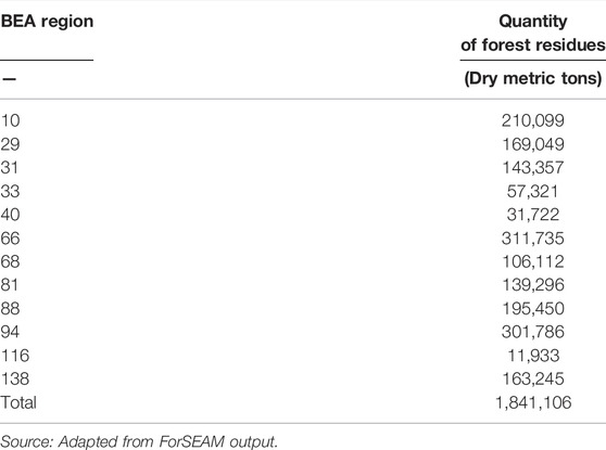
TABLE 4. Location of potential forest residues in the BEAs supplying feedstock to the biorefineries.

BioFLAME Results

Analysis by BioFLAME indicates that enough feedstock is available within the supply area to supply the three biorefineries (Table 5) sited in Morgan County, Kentucky (BEA 94), and Surry and McDowell counties in North Carolina (BEA 31 and 61, respectively) (Figure 4). The cost of the feedstock delivered to the three biorefineries is $104.8 million or about $71/MT (Table 6). This total cost contains costs for the following cost categories: 1. stumpage (∼20 percent), 2. harvest and chipping (∼43 percent), 3. ownership or proprietor income (∼5 percent), and 4. transportation (32 percent) (Figure 5). Transportation of the feedstocks costs about $33.7 million or about $22.70 per dry metric ton (Table 7). Stumpage costs are estimated at about $13.90 per dry metric ton with harvest and chipping cost estimated at $30.30 per dry metric ton.

TABLE 5

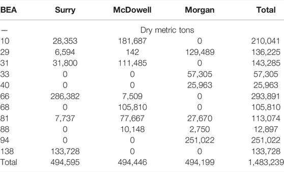
TABLE 5. Quantity of forest residues supplied by BEA.

FIGURE 4

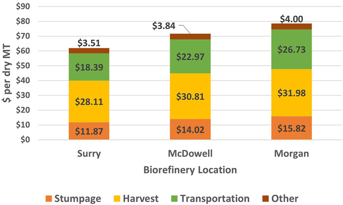
FIGURE 4. Per dry metric ton costs of delivered feedstocks for each of the biorefineries.

TABLE 6

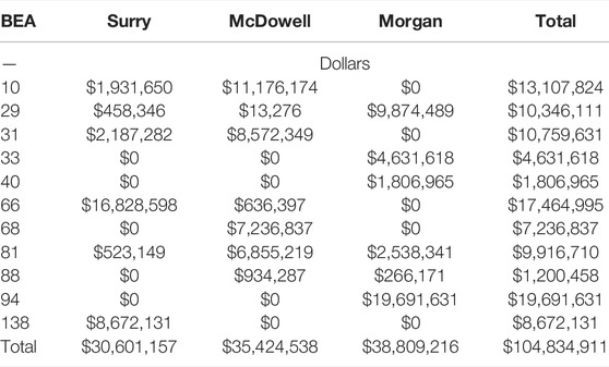
TABLE 6. Cost of the delivered forest residues supplied by BEA.

FIGURE 5

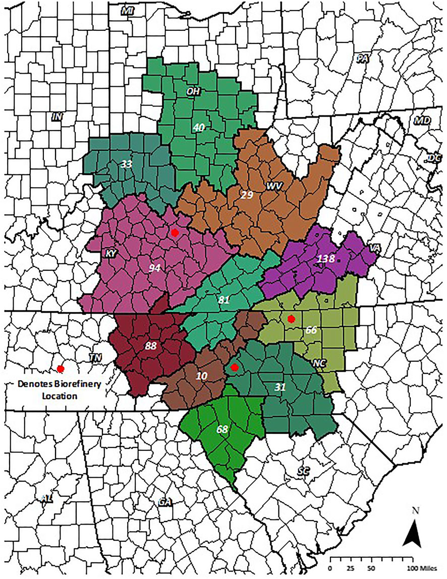
FIGURE 5. Location of the Central Appalachia feedstock draw areas by Bureau of Economic Analysis regions for the gasification and Fischer–Tropsch biorefineries.

TABLE 7

TABLE 7. Cost to transport forest residues to biorefineries by BEA.

Biorefinery Transactions and Output

The biorefinery information used in this analysis data originates from a TEA greenfield gasification Fischer–Tropsch facility spreadsheet with the scale and feedstock costs modified to match the example presented in this article². The facility requires inputs other than feedstock, so those sectors are also impacted. The initial values/assumptions reflect the original development for the United States. The spreadsheet model, once values are changed, calculates the manufacturer’s selling price (MSP) values for all products. Production incentives used in the analysis include RIN values for fuel pathway L given a fuel code of D7 (cellulosic diesel). The prices for fuel code D7 are not available from the EPA’s website, so a D3 (ethanol made from cellulosic material) price series from 2015–2020 is used to establish the estimated RIN value. This value is multiplied by the equivalent value (EV) factor of 1.7 (e-Code of the Federal Regulations (CFR), 2021). The average value of a RIN based on weekly verified observations over December 2019 through August 2020 is 0.32 per liter ranging from $0.13 to $0.47 per liter. When adjusted using the EV factor, the estimated RIN value used in the analysis is $0.55 per liter of advanced fuel (Table 8). The output in liters of sustainable aviation fuel and diesel produced by the biorefineries is obtained from the biorefinery TEA spreadsheet. Naphtha does not have RIN value in this analysis³. Annual production for one biorefinery is 47.5 million liters for SAF, 40.3 million liters for diesel, and 23.6 million liters for naphtha. Both SAF and diesel qualify for RINs. The biorefinery break-even prices required to satisfy investors are estimated at $1.28, $1.32, and $1.13 per liter for SAF, diesel, and naphtha, respectively, for the first biorefinery and $1.37, $1.40, and $1.19, respectively, for the third. The cost differences reflect the changes in feedstock costs delivered to the biorefinery.

TABLE 8

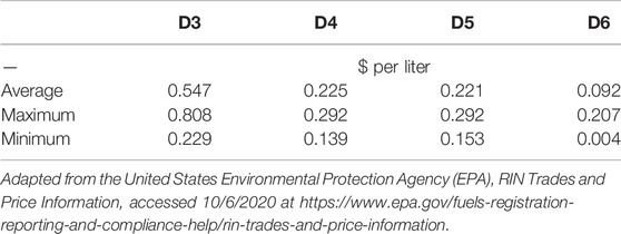
TABLE 8. RIN values increased by the equivalent value BTU adjustment over the last 9 Months, i.e., December 2019 to August 2020.

Capital Costs

The original TEA was developed based on an annual feedstock throughput of 348.5 thousand metric tons with investment costs of $444.6 million (Brandt, Tanzil, Garcia-Perez, and Wolcott, 2021). The designed biorefinery used in this analysis has feedstock throughput of 495 thousand metric tons with an investment cost of $563.6 million (Table 9). The capital costs for the biorefinery include equipment cost, installation of equipment, and working capital required. The equipment costs for gasification ($76.8 million), syngas cleaning ($9.3 million), fuel synthesis ($27.5 million), hydro-processing ($15.5 million), and air separation ($8.8 million) are multiplied by a ratio factor of 4.46 to determine the fixed capital investment for a facility using mature technology ($605.5 million)⁴. Working capital is equal to an additional $14.5 million. The information from the original spreadsheet with a biorefinery throughput equal to 348.5 thousand metric tons was placed into IMPLAN for each BEA in the conterminous United States. Using analysis-byparts (Lucas, 2020), the economic impact resulting from this investment was estimated. The factors were developed based on the investment ratio, actual investment over original investment estimate (563.6/348.5). Therefore, in each BEA that a biorefinery was located, a factor of 1.78 is used to estimate the economic impact of a larger facility and then the original.

TABLE 9

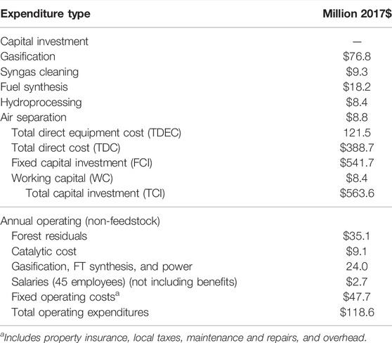
TABLE 9. Summary of capital investment and annual operating costs for the gasification and Fischer–Tropsch conversion facility.

Operating Costs

Operating hours are estimated at 7,884 h per year. Delivered equipment costs are delineated as gasification, syngas cleaning, fuel synthesis, hydro-processing, and air separation and comprise $121.5 (2017$) million of the total capital investments. The remaining costs are based on ratio factors and/or percentages based on information from the plant design and assumptions made for the construction of chemical-based facilities (i.e., total direct cost (3.20), fixed capital investment (4.46), and working capital (20 percent of yearly operating)).

Each biorefinery produces 47.5 mm L/year of sustainable aviation fuel, 40.3 mm L/year of diesel, and 23.6 mm L/year of naphtha. The total feedstock cost delivered to the biorefineries is estimated at $35.1 million (Table 4). An estimated 1.5 million metric tons of dry forest residue are required. However, they are not dried when transported from the field to the biorefinery. Fifty percent moisture content is assumed. Average per ton-mile distance from field to biorefinery is 107 km. The trucks are hauling 18.15 metric tons of chips and 107 km on average. Working 330 days/year and 16 h/day, 31 trucks must be emptied every hour or one truck every 2 min. If they have a longer trailer and can haul 20.4 metric tons of chips, then they need to unload 27–28 trucks per hour. Total feedstock costs arriving at the biorefinery in chipped form average $70.66 per metric ton and include a stumpage fee, harvest and chipping cost, ownership payment, and transportation.

Operating Revenues

Required gross revenues containing a ROI (return on investment) of 12.2% for each of the biorefineries are estimated at $193.7 million from fuel, if $47 million is generated from RINs assuming a RIN price of $0.55 with an energy value (EV) factor of 1.7 for sustainable aviation fuels and diesel. Break-even plant gate fuel price when assuming RINs and a 12.2% on investment are $1.12 per liter for sustainable aviation fuel, $1.15 per liter for diesel, and $0.97 per liter for naphtha. If the output generated from the biorefinery is sold at prices reflected at refineries, then prices reflect the market price and not the price required for sustainable operations.

Generating the Factors

Each stage along the supply chain has a spreadsheet generated for a specific technology, value, and/or size. For instance, the impact for a change in proprietor income is estimated using a million-dollar expenditure within the economy for the proprietor income sector. Transactions resulting from transportation are estimated assuming that they occur from the point of origin and are equal to ten million dollars. A 348.5-thousand-ton biorefinery is assumed and the impact for that sized biorefinery is assumed in the spreadsheets representing that technology. The feedstock transactions are broken into stumpage (proprietor income), harvest costs including chipping, and a small amount for profit. Reestablishment is not assumed, and therefore the costs are not included though these costs would be allocated to a traditional logging operation that leaves the residues behind. The factors are estimated using estimated transactions divided by the direct transactions assumed by the spreadsheet. For instance, if a particular BEA has an estimated eight million dollars in transportation transactions, the factor would equal 0.8 for that BEA. Table 10 contains the factors used to estimate the economic impact for the collection/harvest and delivery of feedstock to the biorefinery. Once at the biorefinery, the factors are based on plant capacity and compared to the expenditures of the modeled facility having a capacity of 348,500 metric tons of feedstock per year. These factors for investment, operating, and salaries are 1.268, 1.325, and 1.271, respectively, for BEAs 10, 66, and 94, the BEA’s where the biorefineries are located.

TABLE 10

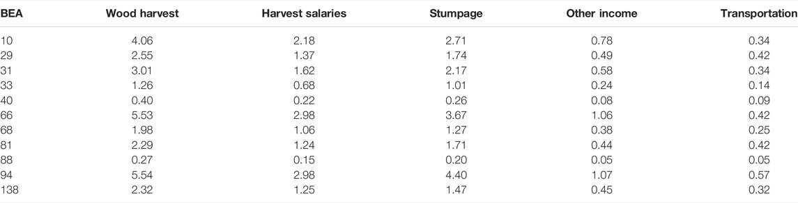
TABLE 10. Factors used to estimate the economic impact from feedstock harvest and delivery to the biorefineries by BEA.

Economic Impact

Based on the IMPLAN-estimated economic impact, the annual economic impact on the Central Appalachian region, if three biorefineries are established, is over half a billion dollars ($537 million per year) based on an investment of $1.69 billion. The investment results in $2.67 billion in economic activity and the multiplier of 1.71. In other words, for every additional million dollars spent, an additional $0.71 million in economic activity is generated in the regional economy (Table 11). The gross regional product is estimated at $1.28 billion from the investment and nearly 200 million each year in annual operating. Each biorefinery employs 47 individuals, but the reverberation of the biorefineries economic activity throughout the BEA regions supports nearly 1,200 jobs because of regional transactions stemming from biorefinery operations.

TABLE 11

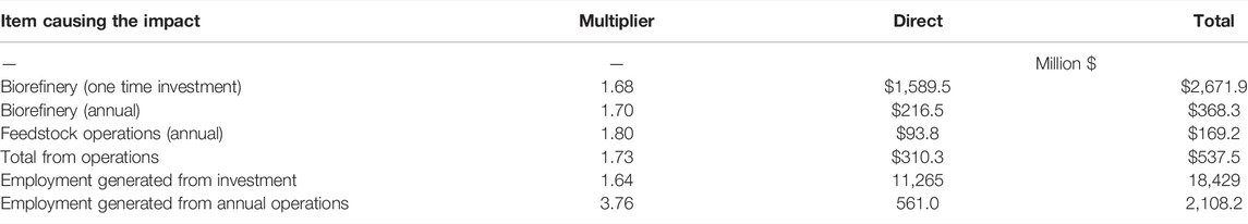
TABLE 11. Total economic activity generated from the three biorefineries.

The feedstock operations also add economic activity to the region. Slightly more than $16.8 million was spent in the harvest and chipping operations (Table 12). This expenditure resulted in an additional $30 million in the economic impact. The stumpage and additional profit occurring from the harvest of the forest residues resulted in $40 million directly into the pockets of the resource and logging operation owners. Their subsequent expenditures resulted in a total economic activity increase of $71.4 million. These operations resulted in creating an estimated 103 jobs directly and a total of 195 jobs. Slightly more than $36.7 million was spent on feedstock transportation resulting in increased economic activity of almost $68 million. The economic activity generated includes the costs of operations, any profit generated, and equipment repair and depreciation along with the multiplier effects that occur after these transactions occur.

TABLE 12

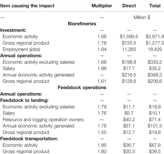
TABLE 12. Economic activity generated by the three biorefinery industry.

Discussion

Based on ASCENT’s GFT conversion techno-economic analysis for sustainable aviation fuel and BioFLAME to simulate the location and transportation of feedstock, this static modeling approach indicates that the biorefinery would need to sell their sustainable aviation fuel at $1.68 to $1.76 per liter, if a required rate of investment is 12.2%. If the hardwood feedstock qualified for RINs, using the average RIN value over December 2019–August 2020 time frame, this break-even price would be reduced to $1.21 to $1.26 per liter assuming a D3 RIN price of $0.32 per liter and an EV factor of 1.7. The economic analysis demonstrates, using GFT technology, to be feasible, the airlines will need to purchase the fuel at a price higher than current levels of aviation fuel or additional subsidies will be required in order to incentivize production. It is estimated that if incentivized, the increase in supply chain expenditures would lead to an annual increase of $600 million through direct expenditures and $1.06 billion after the multiplier effect occurs. In addition, the investment in three biorefineries of $1.7 billion leads to a regional impact of $2.06 billion. The analysis assumes that no additional investment will be required in the logging industry or the transportation industry.

The economic impact in the Central Appalachian region is rather large and given the demise in coal production, could be the new economic engine for the region. The payroll will likely increase by $45 million per year. In 2017, 19 counties within the Central Appalachian region had some of the highest unemployment rates in Appalachia ranging from 8 to 15.7 percent (Appalachian Regional Commission, 2019), whereas the U.S. average during that time period was 4.4 percent. The adoption of this industry will result in additional jobs for the region likely to reduce poverty and out-migration. Families will benefit from the increased economic development as their standard of living increases.

The limitation of input–output models and, certainly a limitation in this analysis, is that the assumptions used are static. They represent a snapshot of the economy at a point in time. Significant change in the demand for inputs might encourage growth of other supporting industries in the region. This change would affect the EIA results. In addition, input–output models are linear, and doubling the output does not change the production function used to determine transactions. Cottage industries that exist may become more efficient as they scale up. Finally, they may overestimate the impact on employment. As suggested by EPA, this occurs since the model does not have resource constraints or substitution effects (Environmental Protection Agency, 2010).

The analysis assumes that mature technology exists to estimate the economic benefits of the biorefineries. The investment, feedstock harvest and delivery, and the operating costs are the estimates. They are not known with certainty. While the technology has been shown to be feasible at the bench scale, a commercial plant has not been constructed yet. Actual costs and economic impacts will likely differ as a result. In addition, the analysis does not include risk except in the assumption that the investment requires a 12.2 percent return. As indicated by Trejo-Pech et al. (2021), this return might not be acceptable.

Data Availability Statement

The raw data supporting the conclusion of this article will be made available by the authors, without undue reservation.

Author Contributions

All authors listed have made a substantial, direct, and intellectual contribution to the work and approved it for publication.

Funding

This work was funded in part by the U.S. Federal Aviation Administration (FAA) Office of Environment and Energy as a part of ASCENT Project 1 under FAA Award Number: 13-C-AJFEUTENN-Amd 13. Funding also was provided by the USDA through Hatch Project TN000444. Any opinions, findings, and conclusions or recommendations expressed in this article are those of the authors and do not necessarily reflect the views of the FAA or other ASCENT-sponsored organizations.

Conflict of Interest

The authors declare that the research was conducted in the absence of any commercial or financial relationships that could be construed as a potential conflict of interest.

Publisher’s Note

All claims expressed in this article are solely those of the authors and do not necessarily represent those of their affiliated organizations, or those of the publisher, the editors, and the reviewers. Any product that may be evaluated in this article, or claim that may be made by its manufacturer, is not guaranteed or endorsed by the publisher.

Acknowledgments

The authors would like to thank Nathan Brown (FAA), Anna Oldani (FAA), and Jim Hileman (FAA) for providing the means to develop the modeling system and Tim Rials (UT) for inviting us to provide feedstock information to ASCENT.

Footnotes

¹Total industry output is defined as the annual dollar value of goods and services that an industry produces. Employment represents total waged and salaried employees as well as self-employed jobs in a region, for the both full- and part-time workers. Labor income consists of employee compensation and proprietor income. Total value added is defined as all income to workers paid by employers (employee compensation); self-employed income (proprietor income); interests, rents, royalties, dividends, and profit payments; and excise and sales taxes paid by individuals to businesses. State/local taxes are comprised of sales tax, property taxes, motor vehicle license taxes, and other taxes.

²Most of the ASCENT TEA conversion facility spreadsheets are developed at Washington State University (WSU). These spreadsheets contain information on a prespecified technology on investment in the facility as well as operations. Currently, these TEAs provide an input sheet and an output sheet, along with information on CAPEX and OPEX (Brandt et al., 2021). The ASCENT technologies available are a portion of the TEAs that have been created and include alcohol-tojet, gasification/Fischer–Tropsch, and HEFA. Since ASCENT technologies focus on SAF, other TEAs are also incorporated into REEAL that focus on the production of other liquid fuels. The ASCENT baseline spreadsheets calculate a minimum selling price for the fuel products produced assuming that a 12.2 percent return on investment is required. These baseline spreadsheets have a specified throughput and cost of feedstock that the user can change.

³Naphtha in not identified as a fuel in approved pathway L. Naphtha is identified as a fuel in several other pathways. These pathways have either a D5 or a D7 fuel code. Had either the D5 or D7 price been used, the estimated selling price required to allow the facility to break even would have decreased.

⁴Mature technology or “nth” plant is assumed for the biorefinery as compared to a “pioneer” facility. The pioneer facility would likely not be as large and therefore would not incorporate economies of scale that potentially exist. In addition, the other aspects of the supply chain are mature. The technologies used to grow, maintain, and harvest the feedstocks, in addition to transporting those feedstocks, are mature or “proven” technologies compared to pioneer technology. Changes in all steps of the supply chain are likely to be different than those modeled.

References

Appalachian Regional Commission (2019). Unemployment Rates in Appalachia, 2017. Baumol, William, 2000. “Leontief’s Great Leap Forward,” Economic Systems Research https://www.arc.gov/map/unemployment-rates-in-appalachia-2017/(Accessed September 20, 2021).

Google Scholar

Baumol, W. (2000). Leontief’s Great Leap Forward: Beyond Quesnay, Marx, and von Bortkiewicz. Econ. Syst. Res. 12, 1. doi:10.1080/0953531005000566241‐152

CrossRef Full Text | Google Scholar

Brandt, K., Tanzil, A. H., Garcia-Perez, M., and Wolcott, M. (2021). GFT_CAEP-v6.xlsm, Excel Notebook. February 4, 2021 email.

Google Scholar

Clouse, D. (2021). ABP: Introduction to Analysis-By-Parts. Available at: https://implanhelp.zendesk.com/hc/en-us/articles/360013968053-ABP-Introduction-to-Analysis-By-Parts (Accessed September 21, 2021).

Google Scholar

De La Torre Ugarte, D., English, B. C., and Jensen, K. (2007). Sixty Billion Gallons by 2030: Economic and Agricultural Impacts of Ethanol and Biodiesel Expansion. Am. J. Agric. Econ. 89, 1290–1295. doi:10.1111/j.1467-8276.2007.01099.x

CrossRef Full Text | Google Scholar

e-Code of the Federal Regulations (CFR) (2021). § 80.1426 How Are RINs Generated and Assigned to Batches of Renewable Fuel? Available at: https://www.ecfr.gov/current/title-40/chapter-I/subchapter-C/part-80/subpart-M/section-80.1426 (Last accessed September 21, 2021).

Google Scholar

English, B. C., Ugarte, D. G. D. L. T., Walsh, M. E., Hellwinkel, C., and Menard, J. (2006). Economic Competitiveness of Bioenergy Production and Effects on Agriculture of the Southern Region. J. Agric. Appl. Econ. 38, 389–402. doi:10.1017/S1074070800022434

CrossRef Full Text | Google Scholar

English, B., de la Torre Ugarte, D., Jensen, K., Hellwinckel, C., Menard, J., Wilson, B., et al. (2006). 25% Renewable Energy for the United States by 2025: Agricultural and Economic Impacts. Accessed at https://ag.tennessee.edu/arec/Documents/AIMAGPubs/BioEnergy/25x25RenewableEnergyAgEcon Impacts.pdf.

Google Scholar

English, B., Jensen, K., Menard, J., and de la Torre Ugarte, D. (2009a). Projected Impacts of Federal Renewable Portfolio Standards on the Colorado Economy. Accessed at https://ag.tennessee.edu/arec/Documents/AIMAGPubs/BioEnergy/ColoradoStudyDocument.pdf.

Google Scholar

English, B., Jensen, K., Menard, J., and de la Torre Ugarte, D. (2009b). Projected Impacts of Federal Renewable Portfolio Standards on the Florida Economy. Accessed at https://ag.tennessee.edu/arec/Documents/AIMAGPubs/BioEnergy/FloridaStudyDocument.pdf.

Google Scholar

English, B., Jensen, K., Menard, J., and de la Torre Ugarte, D. (2009c). Projected Impacts of Federal Renewable Portfolio Standards on the Kansas Economy. Accessed at https://ag.tennessee.edu/arec/Documents/AIMAGPubs/BioEnergy/KansasStudyDocument.pdf.

Google Scholar

English, B., Jensen, K., Menard, J., and de la Torre Ugarte, D. (2009d). Projected Impacts of Federal Renewable Portfolio Standards on the North Carolina Economy. Accessed at https://ag.tennessee.edu/arec/Documents/AIMAGPubs/BioEnergy/NCStudyDocument.pdf.

Google Scholar

Environmental Protection Agency (EPA) (2010). Motor Vehicle Emission Simulator (MOVES3), User Guide for MOVES2010a. Available at: https://nepis.epa.gov/Exe/ZyPDF.cgi?Dockey=P1008EU8.pdf (Accessed September 21, 2021).

Google Scholar

Environmental Science Research Institute (2006). U.S. Detailed Streets. Available at: https://www.lib.ncsu.edu/gis/esridm/2006/usa/streets.html (Accessed August 21, 2016).

Google Scholar

Graham, R. L., English, B. C., and Noon, C. E. (2000). A Geographic Information System-Based Modeling System for Evaluating the Cost of Delivered Energy Crop Feedstock. Biomass and Bioenergy 18, 309–329. doi:10.1016/s0961-9534(99)00098-7

CrossRef Full Text | Google Scholar

He, L., English, B. C., Menard, R. J., and Lambert, D. M. (2016). Regional Woody Biomass Supply and Economic Impacts from Harvesting in the Southern U.S. Energ. Econ. 60, 151–161. doi:10.1016/j.eneco.2016.09.007

CrossRef Full Text | Google Scholar

He-Lambert, L., English, B. C., Lambert, D. M., Shylo, O., Larson, J. A., Yu, T. E., et al. (2018). Determining a Geographic High Resolution Supply Chain Network for a Large Scale Biofuel Industry. Appl. Energ. 218, 266–281. doi:10.1016/j.apenergy.2018.02.162

CrossRef Full Text | Google Scholar

Hellwinckel, C. (2019). Spatial Interpolation of Crop Budgets. Documentation of POLYSYS Regional Budget Estimation. University of Tennessee. Agricultural Policy Analysis Center. Available at: https://arec.tennessee.edu/wp-content/uploads/sites/17/2021/03/POLYSYS_documentation_3_budgeting_database.pdf (Accessed September 21, 2021).

Google Scholar

IMPLAN Group LLC (2018) IMPLAN System (2018 Data and V. 3 Software), Available at: Economic Impact Analysis for Planning | IMPLAN [Accessed September 21, 2021].

Google Scholar

Johnson, K. P., and Kort, J. R. (2004). 2004 Redefinition of the BEA Economic Areas. Available at: https://apps.bea.gov/scb/pdf/2004/11November/1104Econ-Areas.pdf ([Last accessed September 21, 2021).

Google Scholar

Kumar, A., and Sokhansanj, S. (2007). Switchgrass (Panicum Vigratum, L.) Delivery to a Biorefinery Using Integrated Biomass Supply Analysis and Logistics (IBSAL) Model. Bioresour. Techn. 98 (5), 1033–1044. doi:10.1016/j.biortech.2006.04.027

PubMed Abstract | CrossRef Full Text | Google Scholar

Lambert, D. M., English, B. C., Menard, R. J., and Wilson, B. (2016). Regional Economic Impacts of Biochemical and Pyrolysis Biofuel Production in the Southeastern US: A Systems Modeling Approach. As 07, 407–419. doi:10.4236/as.2016.76042

CrossRef Full Text | Google Scholar

U.S. Department of Energy, M. H. Langholtz, B. J. Stokes, and L. M. Eaton (2016). in 2016 Billion-Ton Report: Advancing Domestic Resources for a Thriving Bioeconomy, Volume 1: Economic Availability of Feedstocks (Oak Ridge, TN: Oak Ridge National Laboratory), 448. (Leads), ORNL/TM-2016/160. Accessed at: http://energy.gov/eere/bioenergy/2016-billion-ton-report. doi:10.2172/1271651

CrossRef Full Text | Google Scholar

Larson, J. A., Yu, T. H., English, B. C., Mooney, D. F., and Wang, C. (2010). Cost Evaluation of Alternative Switchgrass Producing, Harvesting, Storing, and Transporting Systems and Their Logistics in the Southeastern USA. Agric. Finance Rev. 70 (2), 184–200. doi:10.1108/00021461011064950

CrossRef Full Text | Google Scholar

Lonergan, S. C., and Cocklin, C. (1985). Use of Input-Output Analysis in Environmental Planning. J. Environ. Manage. 20, 2. U.S. Department of Energy, Office of Scientific and Technical Information, Accessed at https://www.osti.gov/biblio/5390971.

Google Scholar

Lucas, M. (2020). IMPLAN Online: The Basics of Analysis-By-Parts. Available at: https://support.implan.com/hc/en-us/articles/360000814393-IMPLAN-Online-The-Basics-of-Analysis-By-Parts.

Google Scholar

Markel, E., English, B. C., Hellwinckel, C. M., and Menard, R. J. (2019). Potential for Pennycress to Support a Renewable Jet Fuel Industry. SciEnvironm 1, 121. Available at: https://www.hendun.org/viewJournal/RAS211-177/Potential-for-Pennycress-to-Support-a-Renewable-Jet-Fuel-Industry.

Google Scholar

Ralston, S. N., Hastings, S. E., and Brucker, S. M. (1986). Improving Regional I-O Models: Evidence against Uniform Regional purchase Coefficients across Rows. Ann. Reg. Sci. 20, 65–80. doi:10.1007/BF01283624

CrossRef Full Text | Google Scholar

Sharma, B., Birrell, S., and Miguez, F. E. (2017). Spatial Modeling Framework for Bioethanol Plant Siting and Biofuel Production Potential in the U.S. Appl. Energ. 191, 75–86. doi:10.1016/j.apenergy.2017.01.015

CrossRef Full Text | Google Scholar

Trejo-Pech, C. O., Larson, J. A., English, B. C., and Yu, T. E. (2021). Biofuel Discount Rates and Stochastic Techno-Economic Analysis for a Prospective Pennycress (Thlaspi Arvense L.) Sustainable Aviation Fuel Supply Chain. Front. Energ. Res. 9. URL=https://Frontiers | Biofuel Discount Rates and Stochastic Techno-Economic Analysis for a Prospective Pennycress (Thlaspi arvense L.) Sustainable Aviation Fuel Supply Chain | Energy Research (frontiersin.org). doi:10.3389/fenrg.2021.770479

CrossRef Full Text | Google Scholar

U.S. Department of Census (2021). North American Industry Classification System. Available at: https://www.census.gov/naics/(Accessed September 21, 2021).

Google Scholar